MSc Thesis
(Afstudeerscriptie)
written byLuite Menno Pieter van Zelst
(born June 1st, 1980 in Hengelo, Overijssel, Netherlands)
under the supervision ofDr A. Ponse, and submitted to the Board of Examiners in partial fulfillment of the requirements for the degree of
MSc in Logic
at theUniversiteit van Amsterdam.
Date of the public defense: Members of the Thesis Committee:
July 2nd, 2008 Dr P. van Emde Boas Dr B. L¨owe
About half a year ago, Alban Ponse, my thesis supervisor, suggested that the topic of ‘computer viruses’ might prove to be interesting, especially for a theoretician like me. A lot of work has been done in applied research; in comparison the field of virus theory has been gathering dust for the last 25 years.
It must be said that I was not immediately convinced. I have long since felt that threat of viruses is largely artificial; not only to the extent that viruses are artificially created and not a spontaneous occurrence of life. One cannot help but wonder about the apparent symbiotic relationship between the anti-virus indus-try and the creators of computer viruses. After all, the anti-virus indusindus-try stands to lose a lot: the projected market size of security software for mobile phones alone is five billion dollars in 2011 [43].
Moreover, while reading several articles on the theory of computer viruses, I got seriously disgruntled. The theory of computer viruses as it was presented, did not appeal to me. However, the signs were unmis-takable: I only get disgruntled if I am passionate about a subject and do not agree with what I read; perhaps even think of another ways of doing things. My academic curiosity was peeked.
I guess any thesis will in a way reflect the character of the author. Personally I find it satisfying to have my bases covered. The entire first chapter is the direct result of saying to myself: “Ok, this paper I’m reading uses Turing Machines. Let’s first write down a concise definition of Turing Machines”. Of course I hope to convince the reader that I am not a windbag. There is just more to Turing Machines than meets the eye initially. It is true that in this chapter I digress a little from the topic of computer viruses. I truly believe, however, that the topic of Turing Machines is of separate interest to the theoretician, whether he be a logician or computer scientist.
In a way, my initial disgruntlement is expressed in Chapter 2, where I review a prominent modeling of computer viruses. The thesis then culminates in Chapter 3 where I do propose another ‘way of doing things’.
The last six months have been a wondrous academic journey. It was a time of many academic firsts for me. About halfway through, I was invited to submit an extended abstract of this thesis for consideration of the third international workshop on the Theory of Computer Viruses [44]. I was duly accepted as speaker. Thanks to the support of the Section Software Engineering of the Faculty of Science, I was able to travel to Nancy, France and present my ideas. As a result I am invited to submit a 15 page version of this thesis for publication in the Journal of Computer Virology [41]. This version if forthcoming. Being passionate about the results, it is a thrilling experience to convey them to an audience that does research in the same field.
Acknowledgements
I would like to thank my supervisor Alban Ponse for all his help and support. I could not have wished for a more dedicated supervisor. Our meetings were not only productive but also thoroughly enjoyable.
Furthermore, I would like to thank to several authors around the world for their kind replies to my queries. In particular: Fred Cohen, Jack B. Copeland and Jean-Yves Marion. We may at times agree or disagree, academically, but we do so in a spirit of friendship.
The gratitude I feel towards my family, especially my wife Karen and my father, is ill expressed in a few lines. Their love and support have been invaluable.
Luite van Zelst, Utrecht, the Netherlands, June 2008.
Preface i
Introduction v
1 Computing Machines 1
1.1 Introduction to Turing Machines . . . 1
1.1.1 Turing Machines as Quadruples . . . 2
1.1.2 Turing Machines as Finite State Machines . . . 4
1.2 Turing Machines Redefined . . . 5
1.2.1 Turing Machine Tape . . . 5
1.2.2 Turing Machine Computations . . . 7
1.2.3 Turing Machine Equivalences . . . 10
1.2.4 Turing Machines with Multiple Tapes . . . 11
1.3 Persistent Turing Machines . . . 12
1.4 Turing’s Original Machines . . . 13
1.4.1 Turing’s Conditions . . . 15
1.4.2 Relaxing Turing’s conditions . . . 18
1.4.3 Talkative Machines . . . 19
1.5 Universal Turing Machines . . . 23
1.5.1 Universal Turing Machines in Literature . . . 23
1.5.2 Turing’s Universal Machine . . . 24
1.5.3 Universal Talkative Machine . . . 25
1.5.4 Universal Persistent Turing Machines . . . 26
2 Modeling Computer Viruses 27 2.1 Computers . . . 27
2.2 Turing Machine Viruses . . . 31
2.2.1 Modern Turing Machines . . . 32
2.2.2 Turing’s original machine . . . 33
2.3 Cohen . . . 33
2.3.1 Cohen Machines . . . 33
2.3.2 Cohen Viruses . . . 36
2.3.3 Interpreted Sequences . . . 37
2.3.4 Computational Aspects . . . 38
2.4 Universal Machine Viruses . . . 39
2.4.1 Universal Turing Machine . . . 39
2.4.2 Universal Protection Machines . . . 40
2.4.3 Universal Persistent Turing Machine . . . 42
3.2 Recursion Machines . . . 47
3.2.1 Modeling an Operating System . . . 48
3.2.2 Memory access . . . 49
3.3 Recursion Machine viruses . . . 50
3.3.1 Viruses as programs . . . 50
3.3.2 Viruses as functions . . . 50
3.3.3 Recursion Machine Viruses . . . 52
3.4 Discussion . . . 52
Summary 55 A Notational Conventions 57 B Long Formulas 59 Bibliography 61 Books . . . 61
Articles . . . 61
Computer viruses tap into a primordial human fear: that of loosing control. The public fascination with viruses exceeds our fascination with other ways in which we lose control over our computers, for example random hardware faults. A probable cause is the perceived prevalence of computer viruses: one expert website indicates that in March 2008 the ‘NetSky’ virus was at 22 percent (!), although without enlightening the reader what that means [45]. Another reason may be the way that the virus disaster strikes: through infection. We feel that we ought to be able to prevent it.
What simple rules should you and I follow to prevent our computers from being infected? Here is a common view: buy and install a virus scanner, adware scanner, email scanner, firewall, etc. On top of that, we might want to tell a commercial company what websites we visit, in order to prevent visiting ‘suspect sites’. In short, we are willing to hand over our money and our privacy to feel more secure.
Still disaster may strike. And perhaps we have good reason to be pessimistic, for it has long since been established that “virus detection is undecidable”. However, we would like to impress upon you that such a claim is very imprecise and based on a mathematical abstraction. In its entirety, the claim should be read as: “given any machine of infinite capacity and any program, can we decide whether the program is a virus for that machine?” The claim then is that we cannot. This might lead us to be overly pessimistic when we consider the question whether for a specific type of computer we can detect viruses within a specific class of programs.
The claim that virus detection is undecidable is based on one seminal work. In 1985 Fred Cohen wrote his doctoral thesis entitled “Computer viruses”. He was the first to use the words “computer viruses” and he proved the undecidability of virus detection. Cohen based his ‘undecidability’ result on a formal model of computer viruses. In his model, viruses are represented as ‘sequences of symbols’ and computers are represented as ‘Turing machines’. Are these representations appropriate? For if they are not so, Cohen’s undecidability result is on loose ground.
Contents
The purpose of this thesis is to examine the following question: “How can we adequately model computers and computer viruses?”. To that end we ask ourselves: Are computers adequately represented by Turing machines? What ingredients are essential for modeling computers? What are computer programs? What are computer viruses?
We have passed the 70thanniversary of Turing’s famous 1936 article which first introduced a machine we now call the ‘Turing machine’ [28]. Since its publication, the concept of Turing machine has become mainstream and is presented in most computer science textbooks. The fact that every author presents his own flavour of Turing machines has lead to a sense of familiarity and confusion. Usually this is no obstacle: we have come to believe that the differences are inessential. Recently, when the results from this thesis were presented at a workshop, various members of the audience asked: “Why, aren’t all Turing machines essentially the same?”1 We will show in Chapter 1 that such a view is overconfident. To that end we rigorously define our own flavour of Turing machines and discuss what choices can make crucial difference.
1At the third international workshop on the Theory of Computer Viruses (TCV’08), at Loria, Nancy, France [44].
Not only do the two kinds of machines differ in the way they work, we also interpret their ‘computation’ differently. It is a purpose in itself to bring this fact out into the open. Even though it is slightly offtopic with respect to computer viruses, we pursue the investigation of Turing’s original machines. This leads us to propose a new machine model that can unify the perceived view with Turing’s work. We refer to the new machine as a ‘Talkative Machine’.
Other machines that resemble Turing Machines (but are used and interpreted differently) include: ‘Uni-versal Turing Machines’ (UTMs) and ‘Persistent Turing Machines’ (PTMs). As these models have a bearing on the definition of computer viruses, we will lay out the groundwork at the end of Chapter 1.
Does any kind of Turing Machine model modern computers? To answer that question we first have to establish what a computer is, exactly. Unfortunately, that is not a very exact subject matter. In Chapter 2 we will first try to establish the minimal elements any computer model should contain in order to sensibly define computer viruses. We will even tempt the reader to convince himself (herself) that a ‘model of computation’ (such as Turing Machines) is not the same as a ‘model of computers’. From the minimal ingredients of a computer model we will argue that, in general, it is not appropriate to model viruses on the basis of Turing machines.
At this point we can discuss several attempts to do just that: combine viruses with Turing Machines. Our foremost interest is in the work of Cohen [5, 16]. Cohen’s work merits special attention because it is the first academic research into computer viruses. Moreover, his central ‘undecidability result’ is often cited, and so far still stands. Surprisingly, an in depth review of his definitions is untrodden territory.
The fact that Cohen’s work has not yet been thoroughly discussed, has not stopped other authors from suggesting different frameworks for the definition of computer viruses [17, 18, 21, 32, 33]. One avenue of approach can be considered ‘variations on a theme of Cohen’. Among these approaches, we will discuss the definition of viruses based on UTMs [18] and PTMs [33]. We seem to be the first to discuss the Universal Protection Machine (UPM), a Turing Machine based computer model proposed by Cohen in his PhD thesis [5] (and not published elsewhere). We hope that our discussion compels the reader to be convinced that Turing Machines (and their derivatives) are unsuitable for modeling computer viruses.
Computing Machines
1.1
Introduction to Turing Machines
To formalise the notion of computability, Turing introduced a machine we have come to call the ‘Turing Machine’ [28]. The merit of the Turing Machine is that it is easy to grasp the ‘mechanical way’ such a machine could work.
A Turing Machine consists of a tape, a tape head and the machine proper (which we will call ‘control machine’). The tape is infinitely long and consists of discrete ‘cells’, also referred to as ‘squares’. Each cell on the tape can contain a symbol. The tape head is at one cell at each moment, and can move one cell to the left or to the right.1 The tape head can recognize (or ‘read’) the symbol in the cell and write a single symbol back to the tape cell.
The control machine determines what the Turing Machine does. It is a mechanical device that may be constructed inany wayfrom finitely many small parts. The tape head and tape are driven by the control machine (and must be engineered to comply). We can describe the behaviour of the control machine as a set of rules of the form “ifMis in machine stateqand the tape head reads symbolsthen write symbols0, move the tape head one position to the left or right (or stay), and enter into stateq0”.2
To convince you that such a mechanical machine could be build, we have to address the issue of building a tape that is infinitely long. Obviously, we cannot do that. But we can construct a tape that is ‘long enough’, even if we do not know how long it should be. We just make the tape longer every time it turns out it is not long enough.3
A Turing Machine in such mechanical terms does not allow for abstract reasoning. As mathematicians, we abstract from the (mechanical) machine and try to capture its functioning. There are probably as many ways to describe Turing Machines as there are mathematicians. Many descriptions of Turing Machines gloss over the particulars, with the effect that the proofs involving Turing Machines often amount to little more than hand waiving.
We will give a short overview of formalisations of Turing Machines in the literature. Astonishingly, the machines defined in most literature have a very different interpretation from the original interpretation in Turing’s 1936 article. We will need more mathematical machinery to discuss Turing’s interpretation, so we leave this to Section 1.3. For now, we start with one of the earliest works (if not the first) with the now 1A different point of view is that the tape head is at a fixed position and that is the tape that moves under the head. This distinction
is immaterial.
2Turing envisaged machines that can writeormove; he also envisaged machines that must writeandmove or stay. We have no
reason to doubt his claim that the difference is inessential. We choose to define machines that writeandmove or stay, throughout the text.
3We would like to draw a parallel with the Eisinga Planetarium in Franeker, the Netherlands. In 1774, Eise Eisinga build a
common interpretation.
1.1.1
Turing Machines as Quadruples
InComputability and unsolvability(1958) Martin Davis very carefully constructs his ‘Turing Machines’ [1]. He stresses that it is important that
... the reader carefully distinguish between formal definitions and more or less vague explana-tions intended to appeal to intuition, and, particularly, that he satisfy himself that only formal definitions are employed in actual proof.
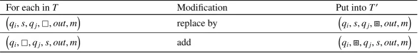
Figure 1.1 depicts how a Turing Machine functions according to Davis. Taking this advise to heart, we now reproduce his abstraction of Turing Machines.
Definition 1.1(Quadruple). Given the sets of symbolsQ= {q1,q2,q3, . . .},Σ = {s0,s1,s2, . . .}andM = {L,R}we define a (Turing Machine) quadruple as qi,sj,A,ql
such that qi,qj ∈ Q, sj ∈ Σ and A ∈ Σ∪ {L,R}.4
Definition 1.2(Turing Machine [1, Definition 1.3]). A Turing MachineZis a finite, nonempty set of (Turing Machine) quadruples that contains no two quadruples whose first two symbols are the same.
Definition 1.3 (Instantaneous description [1, Definition 1.4]). An instantaneous description is a triple (T,qi,T0) such thatT,T0∈Σ∗andqi∈Q. We call the set of all instantaneous descriptionsID.
The ‘Turing Machine’Z is meant to capture the mechanical working of a Turing Machine. The in-stantaneous description is meant to represent the “entire present state of a Turing Machine”, capturing the symbols on the tape, the machine state and the position of the tape head. The tape is represented by two finite strings: T andT0; their concatenation represents a finite part of the tape. To represent a longer part of the tape, the string may grow by concatenating it with symbol s0; this symbol may be thought of as representing a blank square on the tape.
Combining machine and description, Davis defines a transition from one description to the next accord-ing to the rules (quadruples) inZ.5Written asa,→Zb, the transition captures the ‘functioning’ of a Turing Machine.6
On top of these transitions, Davis defines the central notion of Turing Machines: computation.
Definition 1.4(Computation of a Turing Machine [1]). A computation of a Turing MachineZ is a finite sequenceseq:α→IDsuch that:
(∀i< α−1) (seq(i),→Z seq(i+1)) and
(@x∈ID)(seq(α−1),→Z x)
We can introduce short notation for an entire computation by defininga →Z b if and only if there is a
computations:α→IDsuch thata=s(0) andb=s(α−1).
This is one of the points where Davis diverges from Turing’s original approach [28]. Turing start his machine with an empty tape and with the machine in an initial internal state. The above abstract notion of computation leaves us free to choose a sequence with a first instantaneous description that does not represent an empty tape (or has another initial state). We can think of Davis’ ‘non-empty’ descriptions as input. In terms of a concrete mechanical Turing Machine, the input should be written to the tape by some mechanism that isexternal to the machine.
4See [1, Definitions 1.1 and 1.2]. This is an example of a definition that allows the machineeitherto write a symbolorto move,
but not both at the same time. For simplicity, we leave out the fourth quadruple which Davis discusses in chapter 1, section 4 and is intended for the definition of oracle-machines.
Figure 1.1– Three stages of a Turing Machine according to [1]
s1 s1 s1 s1 s0 s0 s0 s0 s0 . . .
s1 s1 s1 s1 s1 s0 s0 s0 s0 . . .
TM Quadruple 1
Quadruple 2 Quadruple 3
. . . Quadruplen
s1 s1 s1 s1 s1 s1 s0 s0 s0 . . .
At the first stage the input on the tape is set to 4 in unary notation.
At the second stage the Turing machine computes. To the left you see the Turing machine at some point during the computa-tion.
At the third stage we read the output 6 from tape.
Figure 1.2– A Turing Machine viewed as a finite state automaton with a tape
q0
q1
q3
q2
q4
0,X,R
Y,Y,R 0,0,R/Y,Y,R
1,Y,L 0,0,L
X,X,R
Y,Y,L
Y,Y,R
,,R
To the left we see a picture of a Turing Machine as automaton (based on an example in [4, Ex-ample 7.1]). It is designed to ‘accept’ an input string of the form 0n1n (n ≥ 1) followed by at
least one ‘’ (blank) symbol.
Davis’ abstraction is an elegant one, because to specify a machine it suffices to specify a finite set of quadruples. We need not specify the sets of state and tape symbols, they are subsumed by the set of quadruples. We can use this to our advantage when we want to compose computations of (possibly different) machines. For example, we can simulate the computation starting from a non-empty tape by a computation starting from an empty tape, using a composition:
→I i→Zr
This composition should be read as: from the instantaneous descriptionrepresenting an empty tape with the tape head at the first square, we can ‘compute’ (by some machineI) the instantaneous descriptionithat serves as input for the computation byZwhich results in a descriptionr.
Finally, Davis gives an example of how to give meaning to a computation. For a computationb →Z c,
ifbandcare of a specific format, we can interpret the computation ascomputing a function(from natural number to natural numbers).
We would like to hold up Computability theoryby Cooper [12] as an example ofhow not todefine Turing Machines. Mostly, Cooper follows Davis’ abstraction, but he does not take Davis quote to heart. Cooper fails to mention instantaneous descriptions or define computations. Most strikingly, Cooper merely claims:
How doesT compute? Obviously, at each step of a computation,T must obey any applicable quadruple.
1.1.2
Turing Machines as Finite State Machines
The most common approach to defining Turing Machines is to view a Turing Machine as a finite-state machine with an infinite tape [2, 4, 9, 10]. The internal ‘states’ of the Turing Machine are regarded as the states of a finite automaton, and the change of state is viewed as a transition. This view allows the authors to express the program (mechanical construction) of the machine as a ‘transition function’ rather than as a set of quadruples.
For Davis the internal states have no intrinsic meaning. Finite state machines, however, may have states that have special meaning, and it is observable that the machine enters into such a state. For example, the transition into a state ‘h’ may be a signal that computation is over. We could also define statesqxthat signal
“the input has propertyx”, or statesqythat signal that the input “does not have propertyy”. The most
com-mon special states are ‘accepting states’ (meaning “the input is accepted”) and ‘rejecting states’ (meaning “the input is not accepted”). Figure 1.2 shows a machine with a single ‘accepting state’.
The definition of such a Turing Machine is along these lines. A machineMis a structure (Q,A,R,H,Σ,Γ,q0) such that:
• Qis a finite set of machine states.
• A⊆Qis the set of ‘accepting states’. If the automaton enters into an ‘accepting state’ the input string is said to have been accepted by the machine; the input string has a certain property.
• R⊆Qis the set of ‘rejecting states’. If the automaton enters into a ‘rejecting state’ the input string is said to have been rejected by the machine; the input string does not have a certain property.
• H⊆Qis the set of ‘halting states’. If the automaton enters into a ‘halting state’ the machine is said to have computed a function on the input string. The symbols that are on the tape at that time, is said to be the output.
• Σis the ‘input alphabet’. Symbols inΣmay be on the tape when the machine is started. • The tape alphabetΓ ⊇ Σ∪ {·
}contains at least the input alphabet and a distinct ‘blank’ symbol.
• q0is the ‘starting state’; when the machine is started the automaton is always in this starting state. • The machine has a transition functiontr⊆(Q\H)×Γ→Q×Γ× move left,stay,move right. Given
a state (not a halting state) and a symbol on the tape it provides a new state (possibly a halting one), a symbol to write on the tape and a direction for the tape head to move.
So far we have only defined a structure, not captured ‘Turing Machine computation’. Unfortunately, some authors do not define computation at all.7 Authors that do define ‘computation’ do so based on their own particular flavour of instantaneous descriptions.8At times computation is called ‘yielding’ [9] or ‘(finitely many) moves’ [4].
1.2
Turing Machines Redefined
We propose to reexamine the definition of a Turing Machine. The authors mentioned in the previous section vary in their definitions on some subtle issues. Do we need a special ‘left-most square’ symbol (as used only in [9, 28])? What is the status of the special ‘blank’ symbol ()? In particular: Should we be able to write blanks? Should we delete trailing blanks after each move (as in [4])? Can (and should) infinite tapes be represented as finite strings?
In this section we will answer such questions. To that end, we will construct a mathematical definition of Turing Machines from the ground up.
1.2.1
Turing Machine Tape
We will start by defining what a Turing Machine tape is, what cells on the tape are, and what content of the cells is. We will draw on the readers mathematical intuitions to support the choices we make. In a general sense we can call the tape a ‘memory’ which consists of infinitely many cells.9We define the memory (and express its infinite size) as:
M is an infinite set (1.1)
Each cell on the tape has content. We call the set of allowed content the ‘base set’ [34]. This will have the same function as the ‘input alphabet’ and is a finite set
B= Σ ={b0, . . . ,bn} (for somen∈ω) (1.2)
We can map each cell on the tape to its content with a total function
S :M→B (1.3)
Different mapsS indicate differences in tape content. For given setsM,Bthe set of all mapsS determines all the possible configurations of the tape:
SM,B={S |S :M →B, S is total} (1.4)
A tape has a left-most cell and with two cellsaandbeitherais ‘to the right of’bor vice versa; therefore we say that the tape is ‘totally ordered’ and that the tape memoryM is countable. This means we can use the ordering of natural numbers to access the tape memory, so there is a bijection:
m:ω↔M† (1.5)
Now we can talk of thenth element of the tape asm(n) and of the content of thenth cell as S(m(n)). However, in view of the fact that this property holds for the tape of any Turing Machine, we disregardM andmand redefine the set of tape configurations so that the content of the nthcell is just written asS(n).
7In this respect [11, Definition C.1] is exemplary, as it only provides the definition of this structure and gives an example of how
the transition function ‘is used’. Even so, the authors feel this is sufficient explanation to go on to state Church’s thesis. To be fair to the authors of this otherwise excellent book, Turing Machines are defined in an appendix, being a side issue to the subject matter.
8Except for [2], where we see only a graphical representation of a part of a two-way infinite tape.
Definition 1.5(Tape configurations). For any base setBthe set of tape configurations is defined as the set of all infiniteB-sequencesSB={S |S :ω→B, S is total}.
We would also like to be able to talk about a cell as ‘not having content’. We do so be stating that a cell contains the special symbol(‘blank’) that is not in the input alphabet. So we change our definition ofB: B= Σ∪ {· }={,b0, . . . ,bn} (for somen∈ω) (1.6)
Using the ‘blank’ symbol, we can define the ‘amount of content’ on the tape as the ‘size’. The intuition is that if there are finitely many non-blank symbols on the tape, there must be a point on the tape where all following symbols are blank.
Definition 1.6(Size). We define the size to be either finite (inω) or infinite (the size isω). size : Bω→(ω+1)
size(S)=minimal n ∈Nempty (1.7)
Nempty=n∈(ω+1)| ∀n0≥n S(n0)=
Note that size(S) is well defined since 1. ω∈Nempty(i.e. it has at least one element)
2. Nempty⊆(ω+1) (i.e. it is well ordered)
Definition 1.7(Finite content). For a tape alphabetΣand base setB= Σ∪ {·
}, we defineFBas the set of
tape configurations with finite amount of content:
FB={S ∈SB|size(S)< ω} (1.8)
The finite content of sequences inFBmay still be scattered on the tape, i.e. there may be blanks before the
last content symbol.
Definition 1.8(Pure content). We say that a tape configuration has pure content if the content is finite and contiguous. We define the set of tape configurations with pure content as
PB={S ∈FB| (∀n< ω) (S(n), ∨n≥size(S))}
There is a bijection between the set of tape configurations with pure content and the set of words (over the same alphabet), as seen in the following lemma. We can interpret this result as: words can be uniquely extended to tape configurations with pure content by adding infinitely many blanks.
Lemma 1.9. Let B= Σ∪ {·
}. ThenPB↔Σ
∗.
P. We define the following functions.
head:PB→Σ∗,
S 7→Ssize(S) ext:Σ∗→PB,
t7→t∪ {(α,) |dom(t)≤α < ω}
Lett∈Σ∗andS ∈
PB. Then
(head◦ext)(t)=head(t∪ {(α,) |dom(t)≤α < ω})
=tsize(t)∪ {(α,) |dom(t)≤α < ω}size(t)
=t∪ ∅=t (ext◦head)(S)=ext(Ssize(S))
=S size(S)∪ {(α,) |dom(Ssize(t))≤α < ω}
=S size(S)∪ {(α,) |size(t)≤α < ω}
=S size(S)∪ {(α,S(α)) |size(t)≤α < ω}
=S size(S)∪ (S \Ssize(t))=S
1.2.2
Turing Machine Computations
We are now ready to define Turing Machines. In the previous section we discussed infinite tapes; this is the first ingredient for Turing Machines. The second ingredient is a set of ‘machines states’. It does not matter what a statereally is; what matters is that we have several. Machines states can be thought of as the machine analogy of human emotions: without fully understanding what the emotions are, we do know that we might do different things depending on our ‘state of mind’.
Definition 1.10(Turing Machine). A Turing Machine is a structure (Q,Σ,tr,q0) whereQis a finite set of states,q0∈Qandtris the transition function:
tr:Q×(Σ∪ {· })→Q×Σ× {−1,0,1} (1.9) The ‘state’ of a Turing Machine is not fully captured by the states inQ, but by ‘configurations’ which we define to be triples (q,t,p) where:
• q∈Qis the current state,
• t∈SΣ∪{·}is the current content of the tape, • p∈ωis the current position of the tape head.
Definition 1.11(Configurations). LetM=(Q,Σ,tr,q0) be a Turing Machine. The set of all configurations ofMis defined as:
CM=(q,t,p) |q∈Q,t∈SΣ∪{·},p∈ω
The transition relation of a Turing Machine determines how a machine goes from one configuration to the next. We call this transition a ‘move’.10 The constraint on the transition is that it respects changes dictated by the transition function: the change of state∈Q, the new tape head position∈ω, and the update of the tape square.
Definition 1.12(Moves). Moves are the binary relation onCMdefined by:
(q,t,p),→M q0,t0,p0 ⇐⇒ tr(q,t(p))= q0,t0(p),p0−p ∧ t0=tp7→t0(p)
The definition of moves only tells ushowtransitions occurs, notwhichtransitions occur. To know that, we have to know which configuration we start out with. In other words: we have to agree how we start a Turing Machine. The first choice to make is: what ‘input’ (or sequence of symbols) is on the tape when the machine starts.
Definition 1.13(Input convention). LetM =(Q,Σ,tr,q0) be a Turing Machine. It is determined by some mechanism external to the Turing Machine (i.e. by us) which is the initial configuration. By convention, the Turing Machine starts in the start stateq0 ∈ Q, the tape head is at the left-most position and the tape contains pure content, which we call the ‘input’. Thus the initial configuration ofMis fully determined by the chosen inputin, written as:
(q0,in,0) for somein∈PΣ∪{·}
R1.14. When we think of the Turing Machine as a mechanical device, the input is placed on the tape by some external mechanism (or person, e.g. by ‘us’). We maintain that such an ‘input mechanism’ is not part of the mathematical definition of the Turing Machine, in a strict sense. Rather, such a mechanism is translated to a ‘convention’ that we should agree upon and adhere to. Admittedly, we could take the view that saying “machineM start with inputin” can be translated to “there is a machineM0that starts with an empty tape, writesinand then performs likeM”. But this is an input convention itself, for it is not in the definition ofMhow to constructM0nor thatM0starts with an empty tape.
We can now ‘start’ a Turing Machine on inputin. Let us see what happens next. Observe that starting a Turing Machine with inputinon the tape, gives rise to a unique sequence of configurations connected by moves. We introduce notation for this sequence.
Definition 1.15(Configuration sequences). LetMbe a Turing Machine andCMbe the set of configurations
ofM. We write seqM(in) for the unique maximal sequence of configurations seqM(in) :α→CMsuch that
seqM(in)(0)=(q0,in,0) ∧ (∀β < α−1) seqM(in)(β),→M seqM(in)(β+1)
What is the length of such a sequence?
Definition 1.16(Computation length). LetMbe a Turing Machine. We write movesM(in) for the length of
the maximal sequence of configurations ofMwith inputin, i.e. movesM(in)=dom(seqM(in)).
Definition 1.17(Halt, diverge). LetMbe a Turing Machine. We say thatMhalts for inputinif movesM(in)<
ω. We say thatMdiverges for inputinif movesM(in)=ω. An alternative (but equivalent) formalisation is
to say thatMhalts for inputinif: (∃α < ω) @c∈CM seq
M(in)(α),→Mc
We would now like to capture a notion of computation. A simple notion is to start the machine with any tape configuration, wait until the machine stops and look at the content on the tape afterwards.
Definition 1.18(Macrostep on tape configurations). LetM =(Q,Σ,tr,q0) be a Turing Machine,B= Σ∪{·
}
andin,out∈SB. We define the binary relation macrostep →M⊆SB×SBby, for someq∈Q,p< ω,
in→Mout ⇐⇒movesM(in)=α+1< ω ∧
seqM(in)(α)=(q,out,p)
The following lemma tells us that from pure content only pure content is reachable. Lemma 1.19. Let M = (Q,Σ,tr,q0) be a Turing Machine, B = Σ∪ {·
}and in,out ∈ SB. The input
convention determines that→M⊆PB×PB.
P. Suppose that in →M outand (by the input convention) thatin ∈ PB. Then by Definition 1.18,
seqM(in)(α)=(q∈Q,out,p∈ω) for someα < ω. Thenout∈PBfollows from the stronger claim that
(∀β < ω) seqM(in)(β)=(q∈Q,t∈PB,p≤size(t))
We prove this by induction onβ.
Supposeβ=0. Then seqM(in)(0)=(q0,in∈PB,0≤size(in)).
Supposeβ=γ+1. Then by Definition 1.15 seqM(in)(γ),→M seqM(in)(β) and by the induction hypothesis
and Definition 1.12:
seqM(in)(γ)= q0∈Q,t0∈PB,p0≤size(t0)
seqM(in)(β)=(q∈Q,t,p)
t0=tp7→x
First of all, sincep0−p∈ {−1,0,1}we havep0≤p+1. • Supposep0<size(t0), then sincet0∈
PB
t=
n,t0(n) |0≤
n<p ∪ {(p,x∈Σ)} ∪
n,t0(n) |p<n<size(t0) ∪(n,
) |size(t
0)≤n< ω
• Supposep0=size(t0), then sincet0∈PB
t=
n,t0(n) |0≤
n<size(t0) ∪ {(p,x∈Σ)} ∪
(n,
) |size(t
0)≤n< ω
From which we may conclude that size(t)=size(t0)+1 and for anyn<size(t) eithert(n)=t0(n)∈Σ ort(n)=x∈Σ. Thent∈PB. Furthermore,p≤p0+1=size(t0)+1=size(t).
By Lemma 1.9 and Lemma 1.19 we can view macrosteps as a relation of words over an alphabet. We will overload the notation of macrosteps.
Definition 1.20(Macrostep on words). LetM =(Q,Σ,tr,q0) be a Turing Machine. We define macrosteps as a relation of words overΣby extending words to tape configuration by adding blanks (see Lemma 1.9):
t∈Σ∗→Mt0∈Σ∗ ⇐⇒ ext(t)→Mext(t0)
So if we stick to the input convention, we can describe distinct tape configurations with words over the input alphabet. That means that we if take a computation (macrostep) from start to finish, we need not concern ourselves with blanks on the tape. We can consider blanks to be part of the black-box functioning of the Turing Machine.
If we allow input fromFB(finite input with intermittent blanks) or if the machine can write blank symbols
(also called ‘erasure’ in the literature) we are in trouble. In both cases ifin→Moutthen in generalout∈FB.
However, we cannot, in general, find the finite content part of a sequence inFB. To that end we would need
more information: we can find the finite part if we can observe how many moves the machine has made since it started computing. (We can use this as an upper bound in our search through the sequenceout∈FB.) We now state our output convention for the record.
Definition 1.21(Output convention). If a Turing Machine halts, the output consists of the entire content of the tape. No other facts about the machine are observable.
We can now interpret Turing Machines as operations on discrete input.
Definition 1.22(Functional interpretation). We say that a Turing Machine M computes the function fM
such that for allin∈Σ∗:
fM(in)=
out if∃out∈Σ∗such thatin→Mout
↑ otherwise
The question arises if this interpretation of Turing Machines completely captures a notion of ‘effective computabilty’. Unfortunately, we cannot claim that every effectively computable function f : Σ∗ → Σ∗is computable by a Turing Machine with alphabetΣ.
R1.23. LetMbe a Turing Machine and fM:Σ∗→Σ∗. We define an ordering onΣ∗bya ≤b ⇐⇒
dom(a)≤dom(b). This ordering compares the lengths of words. Then for any∀a∈Σ∗we have fM(a)≥a.
This is not necessarily true for an arbritrary effectively computable function overΣ∗, for example consider f such thatf(x)7→(whereis the empty string).
Nevertheless, we can compute any effectively computable function of words over subsets of the al-phabet. Or to put it differently: by adding at least one extra symbol to the alphabet we can compute any effectively computable function of words over the original alphabet. In these terms, we can reformulate the Church-Turing thesis:
Conjecture 1.24. For every effectively computable function f : Σ∗ → Σ∗ there is an alphabet Γ with card(Γ) > card(Σ), an (effectively computable) injection in j : Σ∗ → Γ∗ and a Turing-machine M = (Q,Γ,tr,q0∈Q)such that:
We can make the conjecture more specific (and hopefully more intuitive). Conceive of a machine whose alphabetΣis extended with a new ‘erasure’ symboli. Let the input be a word overΣ, but allow the output
to containisymbols. Then the output could be a word overΣof arbitrary length, followed by a number of isymbols. The whole output string is still of greater or equal length as the input string, but theΣsubstring
may be of any (possibly smaller) length. The injection from the previous conjecture is the identity function, its partial inverse is defined as erasing an arbitrary tail ofisymbols.
Conjecture 1.25. For every effectively computable function f :Σ∗ → Σ∗there is a Turing machine M = (Q,Σ∪ {· i},tr,q0∈Q)(and an effectively computable function erase) such that:
f 'erase◦ fM
where
erase(t,n)=
erase(t[n7→],n−1) if t(n)=i∧n>0
t[n7→] if t(n)=i∧n=0
t otherwise
erase(t)=erase(t,dom(t)−1)
Conjectures 1.24 and 1.25 could be viewed as a definition of ‘effective computability’ of functions of words. This view of ‘effective computability’ deviates from the received view: effective computability is a notion about functions on the natural numbers [1, 2, 3, 6, 12]. By coding the natural numbers as words, it can be hypothesized that Turing Machines completely capture the notion of ‘effective computability’. In Chapter 3 we will treat the subject of ‘effective computability’ for functions over domains other the natural numbers.
1.2.3
Turing Machine Equivalences
We say that two Turing MachinesMandNare functionally equivalent if they compute the same function, i.e.:
M≡funcN ⇐⇒ fM' fN (1.10)
In comparing Turing Machines we only look at what we can observe according to our conventions: input and output.11Of course two functionally equivalent machines need not be equal. Thus we are free to define other means of comparison. To do so we have to be explicit about the convention of what is observable, and what is in the black box that is a Turing Machine.
For example, we might state that, in addition to input and output, if a machine stops for some input, it is ob-servablehow manymoves were made since starting. Thus we could compare movesM(in) and movesM0(in) and create smaller equivalence classes. And since movesM(in) also depends oninit allows us to compare
different inputs.
What we cannot do, according to the conventions, is have a peek at the content of the tape while the machine has not yet halted. To allow this, we can define a tape-content-convention. We can get the tape content after each move from the Turing Machine configuration at that point.
Definition 1.26(Tape content convention). LetMbe a Turing Machine andin∈Σ∗. The tape content ofM started withinis observable as the sequence of words tseqM(in) :α→Σ∗
Msuch that:
tseqM(in)(β)=t ⇐⇒ seqM(in)(β)=(q,t,p) (for someq∈Q,p∈ω)
Then tseqM(in)(β) is the content of the tape after βmany moves. We analogously define sseqM(in) as the unique move-connected sequence of Turing Machine states and pseqM(in) as the tape head position sequence.
Using this convention we can look more closely at Turing Machines.
Definition 1.27(Tape equivalence). LetM,N be Turing Machines. Then M andN are tape-equivalent, written asM≡tape Nif:
(∀in∈Σ∗) tseqM(in)=tseqN(in)
Some of the moves connecting the configurations could be viewed as ‘just movement of the tape head’. In our formalisation we cannot distinguish between writing the same symbol to the tape or leaving the cell untouched. There are common formalisations of Turing Machines that do distinguish these, with for exampletr: Q×Σ→ Q×(Σ∪ {−1,· 1}). The drawback here is that a machine cannot write and move the tape head at the same time.
In any case, we like to be able to ‘cut out’ the moves where the tape content does not change. By the tape content convention we already have tape sequences available. We do not need another convention. Definition 1.28(Tape change sequence). LetMbe a Turing Machine andin∈Σ∗
M. We define a tape change
sequences tcseqM(in) as: tcseqM(in) : α→Σ∗M
tcseqM(in)(β)=tcseqM(in)(gM,in(β))
where gM,in(0)=0
gM,in(x+1)=
gM,in(x) if tseqM(in)(x+1)=tseqM(in)(gM,in(x))
g(x)+1 otherwise Now we get our third notion of equivalence.
Definition 1.29(Tape change equivalence). LetM,Nbe Turing Machines. ThenMandNare tape change equivalent, written asM≡changeNif:
(∀in∈Σ∗) tcseqM(in)=tcseqN(in)
We can now express the fact that the (input and output) convention do matter. Claim 1.30. These three equivalence notion are strict refinements in this order:
≡tape⊂ ≡change⊂ ≡func
R1.31. As an example of the importance of the output conventions, we would like to quote from [19,
Section 2.1]. According to van Emde Boas:
If one wants the model to produce output, one normally adopts an ad hoc convention for ex-tracting the output from the final configuration. (For example, the output may consist of all nonblank tape symbols written to the left of the head in the final configuration).
Indeed, the suggested convention allows us to determine a finite output string; in order to do so the tape head position must be observable. While it is perfectly fine to adopt an ad hoc output convention, it would not be fine to omit the convention. The reader may verify that, even for machines that start with input inPB
and that do not write blanks, the functional equivalence derived from this output convention is incomparable to the functional equivalence defined in this section.
1.2.4
Turing Machines with Multiple Tapes
We could conceive of a Turing Machine as having multiple tapes instead of just one. We would like to extend our framework of the previous sections in such a way that the old definitions are a special case. We define ann-tape Turing Machine as a Turing MachineM=(Q,Σ,tr,q0) with the transition function
A configuration is now a triple (q,t,p) such thatq ∈ Q, t ∈ (SB)n and p ∈ ωn. A move is (q,t,p) ,→
(q0,t0,p0) if (q,f rom,q0,to,pos)∈trsuch that:
f rom=(t0(p0), . . . ,tn−1(pn−1))
to=t00(p0), . . . ,t0n−1(pn−1)
pos=(p00−p0), . . . ,(p0n−1−pn−1)
ti0=tipi7→t0i(pi) (for alli<n)
If we extend the input convention to multiple tapes (the initial configuration is (q0,in,0) such thatin∈(PB)n
and0is ann-tuple with all elements zero) then the proof of Lemma 1.19 naturally extends to multiple tapes. That means that with multiple tapes, we can represent the content of each tape with a word over the alphabet. The natural extension of the meaning of Turing Machines follows.
Definition 1.32(Functional interpretation). Letn< ω. We say that an n-tape Turing MachineMcomputes the functionfM: (Σ∗)n→(Σ∗)nsuch that, for allin∈(Σ∗)n:
fM(in)=
out if∃out∈(Σ∗)nsuch thatin→ Mout
↑ otherwise
We can choose to give an n-tape Turing Machine other meaning. For instance, we can only use the first tape for input and output and use the other tapes as ‘working memory’. This can expressed as (f(in)↓ ∧f(in)=out) ⇐⇒ (in, , . . . , ) →M (out,w2, . . . ,wn−1) (where is the empty string and
,w2, . . . ,wn−1,in,out ∈ Σ∗). We can think of other variations, for instance designating some tapes for
input, other for output, etc. In each case we have to be specific about our definitions and conventions. As proved in [9, Theorem 2.1], multiple tape Turing Machines (with the first tape as input/output tape) are equivalent in the sense that for anyn-tape Turing Machine M there is a single tape Turing Machine M0such that fM ' fM0. We have no reason to doubt that this extends to multiple tape Turing Machines as defined in this section. The proof is beyond the scope of this thesis, however.
1.3
Persistent Turing Machines
There is an ongoing debate about the status of Turing Machine computations [26, 36, 38]. Do Turing Ma-chinescaptureall modern notions of computation? Are there notions of computation that are more expres-sive than ‘computing functions’ and yet realistic?
We will now explore ‘Persistent Turing Machines’ (PTMs), which are due to Goldin et al. [26]. Our specific interest in PTMs stems from [33], wherein Hao, Yin and Zhang model computer viruses on (Uni-versal) PTMs. We will discuss to what extent (Uni(Uni-versal) PTMs model ‘computers’ in Section 2.1; we discuss whether they are suitable to define computer viruses in Section 2.4.3. Universal PTMs are intro-duced in Section 1.5.4. In this section we will introduce the reader to the basic definition of PTMs.
Definition 1.33(Persistent Turing Machine). A Persistent Turing Machine (PTM) is a 3-tape Turing Ma-chine (3TM) as defined in Section 1.2.4, where each tape has special meaning:
• The first tape contains the input. In principle, the machine will not write on this tape (this restricts the transition function).
• The second tape is the work tape. The content of this tape is persistent; this is the distinguishing feature of PTMs.
We intend to repeatedly feed the PTM with new input and wait for the output. This process of feeding is meant to be sequential - and the machine may ‘remember’ what input was fed to it. When we say that the content of the work tape is persistent, we mean that in the sequential process of feeding inputs to the machine we leave the work tape undisturbed.
As correctly noted in [36, Section 5.2], a 3-tape Turing Machine can be simulated by a normal (modern 1-tape) Turing Machine. A function computed by a 3-tape machine can be computed by some 1-tape ma-chine. The observation that the authors fail to make, is that if we give new meaning to what the machine does, this new meaning might not be equivalent to the old. Never mind that we use three tapes for a PTM; this just eases the definitions (and our intuitions).
We can formally define PTMs on the basis 3TMs as defined in Section 1.2.4. This is a slight deviation from [26] as our definitions are more restrictive in the use of blanks. (The input and output is restricted to pure content).
Definition 1.34(PTM Macrosteps [26]). LetM be a 3-tape Turing Machine with alphabetΣ. We define
PTM macrosteps−→
M on top of macrosteps of a 3-tape Turing Machine (see Section 1.2.4). Leti,w,w
0,o∈
PΣ∪{·}andbe a tape containing only blanks. Then
w−i−/→o
M w
0 ⇐⇒ (i,w, )→
M i,w0,o
Macrosteps only express the fact that we can feed the PTM a single input. To capture the sequential process that the PTM is meant to carry out, we define PTM sequences. These sequences should capture three notions. First that the input is unknown beforehand (we remain free to choose it). Second, the work tape content is determined by the machine, and is used in the next step. Last, the output is determined by the machine and a given input.
Definition 1.35(PTM sequences). A PTM sequence for machineMis a sequencep:α→(PΣ∗∪{· })
3such thatp(0)=(i, ,o) and for alln< αifp(n)=(i,w,o) andp(n+1)=(i0,w0,o0) then
(i,w, )→M i,w0,o0
Goldin et al. define a ‘persistent stream language’ (PSL) as a sequence of (i,o) pairs, on top of PTM sequences. This leads them to the notion of PSL-equivalence: two machines are equivalent if their language is the same. As PSL-equivalence is strictly larger than functional equivalence (of the underlying 3TMs), Persistent Turing Machines (with the notion of PSL) seem to capture a more fine-grained notion of com-putation. Our intuitions (and hopefully the reader’s intuition) supports this claim: a PTM can deal with an infinite stream of inputs that are unknown beforehand At the same time its ‘memory’ (the work tape) is persistent. It is obvious that such a machine could learn and interact with its environment. Such things are far from obvious for modern Turing Machines with a functional interpretation. For an in-depth discussion of PSL, see [26].
1.4
Turing’s Original Machines
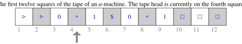
In this section we will discuss the machines that were introduced by Turing’s original article [28]. As we will see these machines are rather different from the modern Turing Machines we have discussed in the previous sections. According to the historical research by Copeland in [13] the best name for these machines is ‘logical computing machines’. Since this name is not well known, we will mostly refer to his machines as ‘Turing’s original machines’ or, in this section, just as ‘machines’. Figure 1.3 shows an example of such a machine.
Figure 1.3– Turing’s original machine
The first twelve squares of the tape of ana-machine. The tape head is currently on the fourth square.
1 2 3 4 5 6 7 8 9 10 11 12
B B 0 ∗ 1 $ 0 ∗ 1
Definition 1.36(machine). A ‘machine’ has the following properties • A machine has finitely many states (or ‘m-configurations’).12
• A machine has a tape divided into squares that can contain one symbol at a time.13
• The machine has a ‘tape head’ that reads one symbol at a time, called the ‘scanned symbol’.14 • The machine makes ‘moves’: go to a new state and erase the symbol, write the symbol or move one
square to the left or right.15
• The possible moves of the machine at any stage are fully determined by the ‘scanned symbol’ and them-configuration. This pair is called the ‘configuration’.16
Definition 1.37(a-machine). If at all stages of movement, the machine has at most one possible move, we call it ana-machine (‘automatic machine’).17
R1.38 (c-machine). If at any stage the machine has at more than one possible move, Turing calls it a
c-machine (‘choice machine’). This choice is determined by something external to the machine.18 Such a machine is closely related to what is commonly known as a ‘non-deterministic Turing Machine’; whereas a-machines can be thought of as ‘deterministic Turing Machines’.
Turing distinguishes two kind of symbols: symbols ‘of the first kind’ (called figures) and symbols ‘of the second kind’. We shall call the second kind ‘auxiliaries’. The auxiliaries are “rough notes to assist the memory” and are “liable to erasure”. Figures, once printed, are not liable to erasure.19
Definition 1.39(Computing machine). A ‘computing machine’ is ana-machine that only prints the figures ‘0’ or ‘1’ (and possibly some auxiliaries).
Definition 1.40(Computed sequence). We say that a machine is ‘properly started’ if it is set in motion from an initial state, supplied with a blank tape. The subsequence of figures on the tape of ana-machine that was properly started, is called the ‘sequence computed by a machine’.
12[28, Section 1]: “We may compare a man in the process of computing a real number to a machine which is only capable of a finite
number of conditionsq1,q2, . . . ,qRwhich will be called ‘m-configurations’.”
13[28, Section 1]: “The machine is supplied with a ‘tape’ [. . . ] running through it, and divided into sections (called ‘squares’) each
capable of bearing a ‘symbol’.”
14[28, Section 1]:“The symbol on the scanned square may be called the ‘scanned symbol’. The ‘scanned symbol’ is the only one of
which the machine is, so to speak, ‘directly aware’.”
15[28, Section 1]: “In some of the configurations in which the scanned square is blank (i.e. bears no symbol) the machine writes down
a new symbol on the scanned square: in other configurations it erases the scanned symbol. The machine may also change the square which is being scanned, but only by shifting it one place to right of left. In addition to any of these operations them-configuration may be changed.”
16[28, Section 1]: “The possible behaviour of the machine at any moment is determined by them-configurationq
nand the scanned
symbol. . . ”
17[28, Section 2]: “If at any stage the motion of a machine [. . . ] iscompletelydetermined by the configuration, we shall call the
machine an ‘automatic machine’ (ora-machine).”
18[28, Section 2]: “For some purposes we might use machines (choice machines ofc-machines) whose motion is only partially
determined by the configuration.[. . . ].When such a machine reaches one of these ambiguous configurations, it cannot go on until some arbitrary choice has been made by an external operator.”
The definition of a ‘computed sequence’ is somewhat unsatisfactory. First of all, it defines a start of moves, but no end. Implicitly, we have to look at the subsequence of figuresin the limit of the moves, i.e. ‘after infinitely many moves’. The question arises if such a subsequence exists (in the limit). Turing remedies this issue with the following (unnamed) convention.
Definition 1.41(Alternation convention). Uneven squares are calledF-squares and even squaresE-squares. A machine shall only write figures on F-squares. “The symbols on F-squares form a continuous se-quence”.20 We call this sequence theF-sequence. Only “symbols onE-squares will be liable to erasure”.
The intuition behind this convention is that each square with ‘real’ content (F-square) is accompanied by an auxiliary square (theE-square to it’s immediate right). The auxiliary squares are just used to make notes to aid the computation.
The alternation convention gives rise to two kind of machines. One: machines whoseF-sequence is finite, called ‘circular’. Two: machines whoseF-sequence is infinite, called ‘circle-free’.21 According to Turing, a machine may be circular because “it reaches a configuration from which there is no possible move, or if it goes on moving and possibly printing [auxiliaries], but cannot print any more [figures]”. Here “configuration” can mean any of three things:
• An ‘m-configuration’: the ‘state’ of the machine.
• A ‘configuration’: the ‘state’ of the machine combined with the scanned symbol.
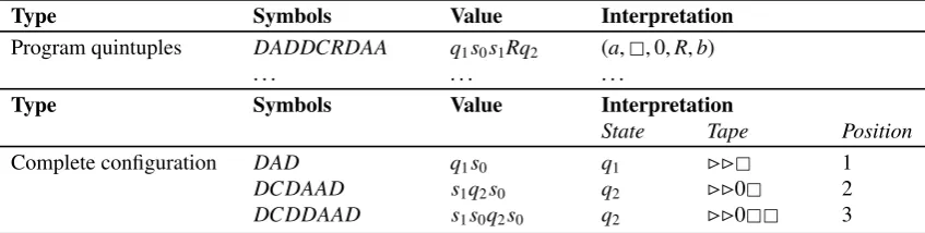
• A ‘complete configuration’, consisting of “the number of the scanned square, the complete sequence of all symbols on the tape, and them-configuration”.
Considering ‘configurations’, we can conclude that Turing allows for machines whose moves are not deter-mined forall m-configurations. In terms of a ‘transition function’: the function may be partial. Considering ‘complete configurations’, we can conclude that Turing, in principle, does not disallow the tape head ‘falling offthe left end of the tape’: if the only possible move on the first square would go to the left the machine breaks down.
The issue of falling offthe left side is addressed by Turing in his second example [28, Section 3]. Although he never explicitly formulates the following convention, his examples stick to it.
Definition 1.42(Left-hand convention). The first moves of a machine printBBon the tape.22 A machine never goes left if the scanned symbol is the leftmostB. A machine never changes or erases aB.
Turing does not explicitly disallow machines to print auxiliaries onF-squares. Once an auxiliary symbol is printed on anF-square, however, it cannot be erased. (This partially supports the left-hand convention.) Notice that thecomputed sequenceand theF-sequence are not exactly the same: thecomputed sequence is the figures-subsequence of theF-sequence. Either sequence can only become longer. Therefore, if a machine is circle-free and obeys the alternation convention, then the computed sequence is guaranteed to exist in the limit of the moves.
1.4.1
Turing’s Conditions
Summarizing the previous section, Turing’sa-machine is subject to the following conditions. 1. Figures can only be written onF-squares.
2. Fsquares are ‘write-once’ (not “liable to erasure”). 3. TheF-squares form a continuous sequence.
20Where ‘continuous’ means: “There are no blanks until the end is reached”.
21[28, Section 2]: “If a computing machines never writes down more than a finite number of symbols of the first kind, it will be
called ‘circular’. Otherwise it is said to be ‘circle-free’ .”
22Turing uses the symbol ‘ e ’. His examples consistently use two such symbols at the start of the tape, even though one would
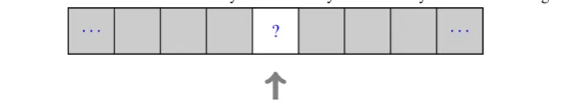
Figure 1.4– The move of a machine is only determined by the current symbol andm-configuration.
. . . ?? . . .
4. The firstF-square and firstE-square contain an ‘B’ symbol that signals the left end of the tape. The
Bsymbol is also ‘write once’. The machine should not move to the left when it reads the leftmostB
symbol.
In the definition of Turing’s machine, we stated that the possible moves of a machine are determined by the configuration (scanned symbol andm-configuration). A move is now (re)defined (in accordance with [28, Section 5]) as consisting of three things: anm-configuration (state) the machine transitions to, a symbol that is to be printed on the current scanned square, and a direction for the tape head to move to. Erasure is expressed as writing a ‘blank’ symbol (). We can think of ‘the moves of ana-machine being determined’ as a transition function.
Definition 1.43(Transition function). The moves of ana-machine are determined by a ‘transition function’ tr. LetQbe the set ofm-configurations (states),Fthe set of figures,Athe set of auxiliaries andL,N,Rbe the possible movements (left, no movement, right). Thentris defined as:
tr:Q×(F∪· A)→Q×(F∪· A)× {L,N,R}
When we write down the function as a list of quintuples, we call it a ‘program’.
Can we determine if an arbitrary function is a ‘valid’ program, i.e. satisfies Turing’s conditions? If we ‘run’ the machine (defined by the program) and it violates the conditions, we know that the function is not a valid program. But how can we be sure that it willneverviolate a condition? We would like to express Turing’s conditions as a property of the transition function, without having to run the machine. We shall now show, however, that this is not possible.
Let us regard the transition function (program) decoupled from the tape. It its most unrestricted form we have a transition functiontr: Q×Σ→Q×Σ× {L,N,R}(directly mirroring Turing’s quintuples). We assume without loss of generality thattris a total function (for each partial function there is an equivalent total one w.r.t. computable sequences). Thus the result of the transition function is fully determined by the input: the current state and the symbol on the scanned square. Notably, we do not give the position of the tape head as input to the function. From the point of view of the transition function, the tape extends arbitrarily many squaresto both sides. This situation is depicted in Figure 1.4.
In order to satisfy Turing’s conditions, we have to distinguish at least six (two times three) situations: • Is the tape head positioned on aF-square orE-square?
• Are we in one of three positions:
– On the leftmost blankF-square? The machine is allowed to write on theF-square.
– To the left of the leftmost blankF-square? The machine is not allowed to write on anyF-square until we move enough squares to the right to reach the leftmost blankF-square.
– To the right of the leftmost blankF-square? The machine is not allowed to write on anyF -square until we move enough -squares to the left to reach the leftmost blankF-square.
Figure 1.5– Blank tape with left hand markers and distinctFandEmarkers.
B B− . . .
Figure 1.6– A machine with a distinct ‘left most blank symbol’.
. . . . . .
the conditions “left of”, “on the leftmost blank” and “right of”; similarly, letqE,l, qE,b, qE,r ∈ Q0be the
three states that signify being on anE-square.
We should then add the appropriate transitions to keep track of the changes of situation; for example if the tape head moves to the rightqF,rshould transition to qE,r. So every move causes a change in state
since the tape head moves from an E-square to an F-square or vice versa. Only now can we check if the transformed function satisfies the conditions. We can guarantee a correctF-sequence if the transition function is the identity function w.r.t. the scanned symbol, if the machine is in the statesqF,landqF,r.
You may have noticed that we could do with less states if we also look at the information carried by the current symbol. For example, we could do with 2 x 2 states by purging the 2 states for “On the leftmost blankF-square”. It is enough to know that we are “not to the right of the leftmost blank F-square”and the current square is blank. In any case, for an arbitrary program, the states do not carry all this information.
Do the symbols on the tape carry the needed information? Let us denote the set of symbols that may appear on theF-squares andE-squares byAF ⊃F andAE ⊃ Arespectively. For any auxiliary that we
wish to write on anF-square (notablyB) we can introduce a new symbol that we only use forE-squares, and use the original forF-squares. In essence, we may assume thatAE andAF are disjoint. Let us at least
distinguish betweenF-blanks () andE-blanks () (similarly for left-hand markers:BandB−respectively). SoAF ⊇F∪ {,B}andAE=A∪ {,B−}. Figure 1.5 exemplifies this idea.
Now if we encounter anF-blank we still have to distinguish between the left-mostF-blank and other F-blanks. Suppose we can and that the left-mostF-blank is marked by a new symbol. This symbol can appear on the tape only once. So if we are in the situation depicted by Figure 1.6, we have sufficient information to know that the machine may write an output symbol. This leaves us with one problem: once the machine writes over the symbol, we have noleft on the tape, so we do not have a marker for the left most blank symbol on the tape. In fact, we cannot place the marker again because we have lost track of its position.
Wrapping up: by making the symbols forF-squares distinct from those onE-squares we have a partial solution. Since the states do not necessarily carry any information, we can not express Turing’s conditions as properties of the configuration, and therefore of transition functions.
We envisage several solutions.
1. We can provide the transition function with more information.
If we let the sets of symbols forF- andE-squares be disjoint, we only have to provide the function with exactly enough information:truefor being on the left-most blankF-square andf alseotherwise. This seems to defeat the purpose of the separation of program and tape: we can only provide the value of this Boolean by keeping track of the ‘complete configuration’ (including the whole tape content and tape head position). Nevertheless, let:
tr:Q×(AF∪· AE)× {true,f alse} → Q×(AF∪· AE)× {L,N,R}
Boolean is correct): tr(qi,,f alse)=
qj,,m
tr(qi,s,b)=
qj,s0,m
such that eithers,s0∈AF ors,s0∈AE tr(qi,s,b)=
qj,s,m
ifs∈ {B,B−} tr(qi,B,b)=
qj,B,m
, such thatm,L
tr(qi,s,b)=
qj,s,m
ifs∈AF
2. We can restrict the movement of the tape head on blankF-squares so that a machine can only move to the right if it writes a non-blank symbol. Let:
tr:Q×(AF∪· AE)→ Q×(AF∪· AE)× {L,N,R}
Then the following restrictions ensures that such a machine adheres to Turing’s conditions: tr(qi,)=
qj,s,m
such that eitherm,Ror (m=R∧s,)
tr(qi,s)=
qj,s0,m
such that eithers,s0∈AF ors,s0∈AE tr(qi,B)=
qj,B,m
, such thatm,L
tr(qi,s)=
qj,s,m
ifs∈ {B−} ∪AF
This approach has the drawback that we cannot write on anE-square without having written to allF -squares to its left. It is unclear if machines with this restriction are as expressive as Turing’s original machines.
We propose a third alternative in the next section.
1.4.2
Relaxing Turing’s conditions
We shall drop all of Turing’s conditions but one. We still enforce the condition that the F-squares are write-once. Now the question arises if the class of such machines also characterises the set of computable sequences. Clearly, the set of all such machines is a superset of the set of machineswithTuring’s condi-tions, so the corresponding set of computable sequences contains at least the set of computable sequences according to Turing. We need only be concerned if such machines do not compute more sequences. That all depends on the interpretation of machines. Turing only gives meaning to ‘circle-free’ machines, the meaning of ‘circular’ machines is undefined.
Definition 1.44(Computable sequence). “A sequence is said to be computable if it is computed by a circle-free machine.” [28, Section 2]
By prescribing thatF-squares are write-once, we ensure that theF-sequence always has a continuous (though possibly finite) initial segment, even in the limit of infinitely many moves. We will use that prop-erty later on. If, in the limit, there are still intermittent blanks in theF-sequence (i.e. the initial continuous segment is not infinite), the machine does not compute a sequence according to Definition 1.44. We need not, therefore, be concerned about such machines. What if, in the limit, the machine does produce a proper continuous, infiniteF-sequence? We have to prove that we can find an equivalent machine that adheres to Turing’s conditions and produces the same computed sequence.
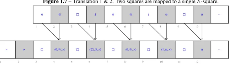
Suppose we have a machine M with the relaxed condition. We will create a new machine from
M. The first step is to translate to a machine M0 that does all the computation on the E-squares and leaves theF-squares intact. We have to explode the set of symbols. We define a set of symbolsAT =
(AF×AE×AM)∪· F∪ {· ,,B,B−}whereAM={∗,×}.
23 The set
AMis used later on as a Boolean marker.
23The set
ATis not a ‘flat’ set of symbol; we could however choose a real set of symbolsA0T that is in bijection withAT. For
![Figure 1.1 – Three stages of a Turing Machine according to [1]](https://thumb-us.123doks.com/thumbv2/123dok_us/8386562.322110/15.595.99.490.167.387/figure-stages-turing-machine-according.webp)