The commodity price and exchange rate dynamics

ISSN Print: 2162-2078

DOI: 10.4236/***.2017.***** **** **, 2017 1 Theoretical Economics Letters

The Commodity Price and Exchange Rate

Dynamics

Liping Zou

, Boliang Zheng

, Xiaoming Li

1_{School of Economics and Finance, Massey University, Auckland, New Zealand}

2_{School of Accountancy, Jiangxi University of Finance and Economics, Nanchang, China}

Email: *[email protected]

Abstract

This paper investigates the dynamic relationship between the commodity price and the exchange rate in Australia and New Zealand. We focus on

Aus-tralia and New Zealand. Not only do their primary commodities account for

significant shares of their exports, but also their currencies share some dis-tinctive characteristics that are unique from other commodity currencies. Us-ing country-specific commodity price indices, we examine the relationship between the departure of currency value from its fair value and fundamental macroeconomic variables. Evidence of a strong and robust relationship be-tween the exchange rate and the commodity price has been found. Results in-dicate that the commodity price can be used to improve the forecast ability of the future exchange rate. Our commodity-price-augmented exchange rate

fo-recasting model consistently outperforms the random-walk model, for both

in-sample and out-of-sample forecasting. These results shed some extra lights on policymaking for countries that rely on primary commodity production, and attempt to move towards floating exchange rate regimes as part of their global market liberalization process.

Keywords

Exchange Rate, Commodity Price, Forecasting

1. Introduction

In past few decades, many attempts to investigate the relation between funda-mental macroeconomic variables and exchange rates have been proven to be failed, not to mention numerous unsuccessful endeavours that economists have made on building various types of exchange rate forecasting models. In early 1970s, after the post-war Bretton Woods system of fixed exchange rates

col-How to cite this paper: Author 1, Author 2 and Author 3 (2017) Paper Title. Theo-retical Economics Letters, 7, *-*.

https://doi.org/10.4236/***.2017.*****

Received: **** **, *** Accepted: **** **, *** Published: **** **, ***

Copyright © 2017 by authors and Scientific Research Publishing Inc. This work is licensed under the Creative Commons Attribution International License (CC BY 4.0).

http://creativecommons.org/licenses/by/4.0/

DOI: 10.4236/***.2017.***** 2 Theoretical Economics Letters

lapsed, a large number of industrialized economies shifted to floating exchange rate regimes. Thus, lots of interests have been put on foreign exchange markets studies. Majority of these work focused on the development of macroeconomic variables based empirical models when forecasting future exchange rates. Meese and Rogoff [1] [2] concluded that there are no exchange rate forecasting models

that could outperform a simple naïve model, i.e. a random walk model, for short

to medium time horizons. Subsequent attempts have been undertaken to de-velop a suitable model to forecast exchange rate, but many failed to do so. Therefore, a simple random walk model has become a benchmark when evalu-ating exchange rate forecasting performance.

Recent literatures on exchange rate determination and forecasting are in line with the propositions found decades ago. Many empirical results conclude that the exchange rate follows a random walk process, changes in exchange rate are unpredictable and currencies for high-inflation countries tend to depreciate in long term with the magnitude being approximately the inflation differential. Movements of the actual exchange rate appear to be sometimes overshot and then followed by a smooth adjustment to the equilibrium [3] [4] [5] [6].

There has been a strand of research investigating countries with differing ex-change rate regimes and economic structures. In particular, countries with “Commodity Currencies” have been given more attentions, evidences have been found that there exists a long-run relationship between the real exchange

rate and the real commodity price for commodity-exporting countries1 _[7],

in-cluding Australia, Canada, Chile, New Zealand2_{, and South Africa. Similar}

re-sults are confirmed by Chen and Rogff [8] for Australia, Canada and New Zea-land. In addition, Chen [10] found that for three major OECD (The Organiza-tion for Economic CooperaOrganiza-tion and Development) primary commodity produc-ers (Australia, Canada, and New Zealand), nominal exchange rates exhibit a ro-bust response to movements in prices of their corresponding commodity prices. Chen and Rogff [11] then subsequently identified two countries from the OECD regime—Australia and New Zealand, as the “exceptions to the rule” when con-sidering exchange rate determination and forecasting. They confirm and extend previous findings that for major commodity exporters with market-based ex-change rates, the price of their primary commodity exports is an important and robust determinant for the real exchange rates. However, the commodity price itself tells little about subsequent exchange rate movements. But when combin-ing various macroeconomic fundamentals with the commodity price, results suggest that it can help to predict quarterly exchange rate changes, however, no single specification emerges as the clear winner across both countries and time period. Other literatures for selective developed and developing nations looking at the same issue include: Amano and van Norden [12], Gruen and Wilkinson 1_{For countries that are heavily relied on commodity products to gain export earnings, the price}

movements in the world commodity markets would then be the changes in the relative demands for their corresponding currencies.

2_{For New Zealand in particular, it refers to Luo and Plantier [9], which focuses on the persistence of}

DOI: 10.4236/***.2017.***** 3 Theoretical Economics Letters

[13], De Gregorio and Wolf [14], Chinn and Johnston [15], and Montiel [16]. However, none was able to offer conclusive evidence to answer why these com-modity currencies are unique and may require further investigation. Therefore, our study serves to answer these questions.

Australia and New Zealand are two open economies in the OECD regime. They both share a number of distinctive features in economic structures and policy settings. These special features have made the two nation’s currencies demonstrate a remarkable strong “commodity currency phenomenon” and to

stand out among other commodity currencies3_{. Australia is an export-oriented}

economy, whose exports in primary commodity products take a significant por-tion of their gross domestic producpor-tion. Characterized by mainly mineral (or “hard”) commodity exporting, the primary commodity products exported by Australia include iron ore, metallurgical coal, thermal coal, gold and various other metal products. These non-energy products, along with other commodities account for more than 60% of Australian total exports. New Zealand, in con-trast, its exports are heavily dependent on agricultural products such as dairy products, wools, meats and other “soft” commodities. Commodity products ex-porting contribute about 67% of its total exports in the late 80s. Primary com-modity products still take about 50% of New Zealand’s total exports today. Moreover, New Zealand is a well-known key player of its commodity products in the global market, in spite of its relatively small economy. It supplies nearly 50% of the total world exports of lamb and mutton where only a fraction of less than 20% of its meat production is consumed domestically. Given both countries are heavily dependent on commodity products to gain export earnings, the price movement in world commodity market would then have an impact on the rela-tive demand for the corresponding currency. Neither of the two countries is big enough to influence the world market, they both also have adopted a sufficiently

long period of a floating exchange rate regime under the inflation targeting

sys-tem4_{, central banks normally have very limited controls and interventions over}

exchange rate movements. Commodity price fluctuations can then essentially represent a source of exogenous shocks to their terms-of-trade, which eventually channel up and trigger the exchange rate responses. Therefore, the introduction of the country-specific commodity prices indices in Australia and New Zealand’s commodity exporting in early 1980s, has offered an opportunity to identify and measure exchange rate fluctuations using these indices.

Motivated by Chen and Rogff [8] [11] studies, we try to investigate if move-ments in commodity prices can explain the fluctuation in exchange rates. We develop an exchange rate forecasting model by putting the commodity price into the structural forecasting model and to examine if this improves the accuracy of 3_{Cashin, Cespedes, and Sahay [7] have classified 58 countries as the “commodity economies” that}

have a significant commodity dependency. In addition to Australia and New Zealand, these coun-tries include Finland, Iceland, Norway, and numerous other developing councoun-tries.

4_{Australia and New Zealand abandoned their exchange rate pegs in 1983 and 1985, respectively, as}

DOI: 10.4236/***.2017.***** 4 Theoretical Economics Letters

exchange rate forecasting. A three-step process is followed in this paper: firstly, we test if the country-specific commodity price index has explanatory power when modelling exchange rates movements in Australia and New Zealand. Our results indicated that the country-specific commodity price index does have some explanatory power and our results are robust. We therefore conclude that the commodity price index should be considered as one of the determinants when forecasting exchange rates. Secondly, we use the cross-rate between Aus-tralian Dollar and New Zealand Dollar to examine the relationship between the cross rate and the commodity price. Results indicate that the commodity price offer an exceptional explanatory power when forecasting the cross-exchange rate movements. Thirdly, once including commodity prices index into the forecast-ing model, the forecastforecast-ing performance of the modified model can be evaluated both in-sample and out-of-sample against a simple random walk model. Our results suggest a remarkable in-sample forecasting performance. For out-of-sample forecasts, the modified exchange forecasting model is also able to provide more consistent forecasting performance than the benchmark random walk model. Therefore, our study contributes to the existing literatures that the commodity price is an important determinant of the current exchange rate and the future exchange rate movements in Australia and New Zealand.

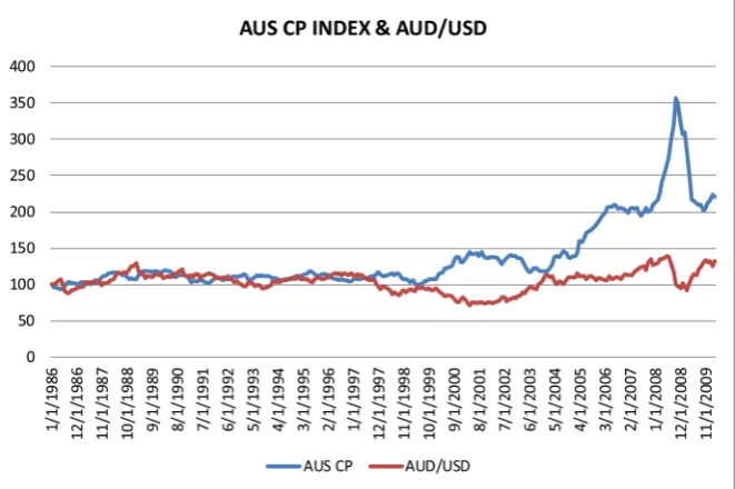
2. Commodity Price Indices in Australia and New Zealand

Figure 1. Relationship between the Australian Commodity Price and the Value of Aus-trian Dollar. Figure 1 illustrates the relationship between the Australian commodity price and the value of Australian Dollar from 1986 to 2010, the base level is set at 100 as of January 1986.

5_{See Appendix A for more information about the commodity indices in Australia and New}

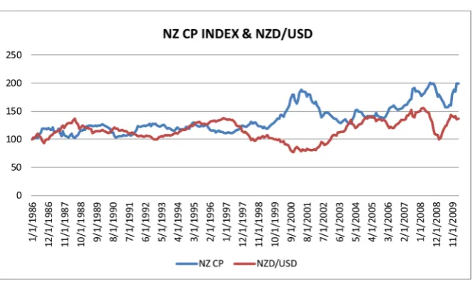
DOI: 10.4236/***.2017.***** 5 Theoretical Economics Letters Figure 2. Relationship between the NZ Commodity Price and the Value of NZ Dollar. Figure 2 illustrates the relationship between the NZ commodity price and the value of New Zealand Dollar from 1986 to 2010, the base level is set at 100 as of January 1986.

Australian and New Zealand commodity price index and their corresponding quoted exchange rate against US dollar from 1986 to 2010, respectively. The commodity index is the monthly time series and its base value is set at 100 as of

1st _{January 1986.}

In Figure 1, we observe that the Australian commodity price and the AUD/USD exchange rate appear to have an inverse relationship. This suggests that when the commodity price is moving up, the AUD/USD exchange rate is going down. Thus, Australian dollar is appreciating when the Australian com-modity price goes up. This implies that the value of the Australian dollar is moving in line with prices of its commodity exporting. Similar pattern is ob-served from Figure 2 for New Zealand. The New Zealand commodity price in-dex also appears to have an inverse relationship with the value of its currency,

especially after late 1990s6_.

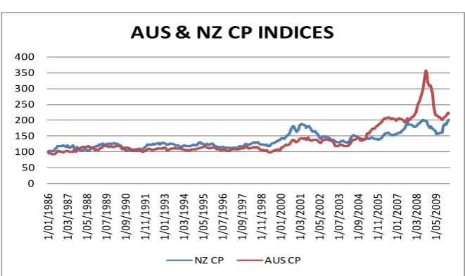
Figure 3 below illustrates the relationship between Australian and New Zea-land commodity price indices. The nature of the underlying commodities which two indices represent is fundamentally different. However, the commodity prices in Australia and New Zealand are having a high level of co-movements from mid 1980s to early 2000s. From late 1990s to 2004, the price of New Zea-land soft commodities enjoyed a relatively higher growth rate compared to Aus-tralian commodity prices. However, with the increasing demand for metal products from developing countries (China in particular) and global economic expansions, Australia has enjoyed the rapid growth in their commodity prices since 2005.

Previous studies have found that some economics models, i.e. PPP, UIP, can

only provide valid information when forecasting exchange rates in the long run. Results from these models usually are not better than a simple random walk

DOI: 10.4236/***.2017.***** 6 Theoretical Economics Letters Figure 3. Relationship between NZ and Australian Commodity Prices. This figure illus-trates the relationship between the commodity price in Australia and New Zealand over time, the base level is set at 100 as of January 1986 for both countries.

model. Since the term “Commodity Currency” has been introduced and brought to the attention of international finance, researchers have found some promising evidences that commodity price may play some roles in determining and

fore-casting exchange rates7_{. A recent study by Luo and Plantier [9] has estimated the}

half-life of NZD/AUD cross rates deviation is about 0.6 years (the time it takes for actual exchange rate to return to its theoretical fundamental value, in this case its PPP value). Whereas a study conducted by Chen and Rogoff [8] reports a more than 1.6 years half-life for the NZD/USD pair and an average of 3 to 5 years reported for various pairs of the commodity currencies in simple PPP-based regression models.

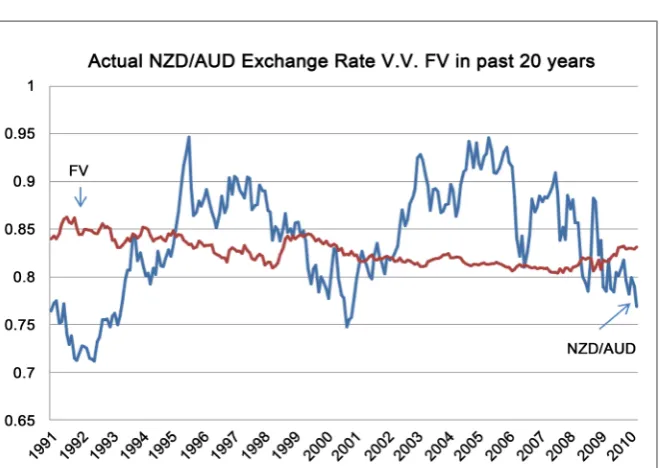
If a random walk is what the exchange rate movement follows, then effects of innovations on the exchange rate are highly persistent and the time series can fluctuate without bounds [7]. Figure 4 below presents the exchange rate behav-iour of NZD/AUD cross rate from 1991 to 2010. The graph indicates that the

actual exchange rate moves within the 10% bounds of its “Fair value”8 _for

major-ity of the sample period. Moreover, there is a clear tendency of the actual cross- exchange rates to return to their long-term “Fair Value” over time. Since the “Fair Value” is usually determined by fundamental macroeconomic variables, it is therefore reasonable to believe that NZD/AUD cross rates may be predicted if shocks are identified and included into an exchange rate forecasting model with possible structural breaks.

In Figure 4, the NZD/AUD long-term “Fair Value” (or the long-term “Equi-librium Value”) is within the 0.8 and 0.85 NZ dollar per Australia dollar range in the past 20 years. The actual exchange rates, on the other hand, fluctuate from as

0 50 100 150 200 250 300 350 400 1/ 01 /1 98 6 1/ 03 /1 98 7 1/ 05 /1 98 8 1/ 07 /1 98 9 1/ 09 /1 99 0 1/ 11 /1 99 1 1/ 01 /1 99 3 1/ 03 /1 99 4 1/ 05 /1 99 5 1/ 07 /1 99 6 1/ 09 /1 99 7 1/ 11 /1 99 8 1/ 01 /2 00 0 1/ 03 /2 00 1 1/ 05 /2 00 2 1/ 07 /2 00 3 1/ 09 /2 00 4 1/ 11 /2 00 5 1/ 01 /2 00 7 1/ 03 /2 00 8 1/ 05 /2 00 9

AUS & NZ CP INDICES

NZ CP AUS CP

7_{For more comprehensive background information and empirical evidences, see Chen [10], Chen}

and Rogoff [11], Chen, Rogoff and Rossi [17].

8_{The fair value is defined as the exchange rate that would be predicted according to PPP and UIP, as}

DOI: 10.4236/***.2017.***** 7 Theoretical Economics Letters Figure 4. The NZD/AUD Exchange Rate and the Corresponding “Fair Value”. This fig-ure illustrates the NZD/AUD cross exchange rate over time. It also presents the ‘Fair Value’ of the cross rate determined by fundamental macroeconomic variables. The hori-zontal axis represents the value of New Zealand dollar per Australian dollar.

high as 0.7 around 1992 to as low as 0.95 in 1995 and 2005. In addition, the fair value appears to be relatively constant overtime and failed to pick up any major ‘break’ of actual exchange rate movements. The lacking correlation between the nominal exchange rate and its underlying long-term equilibrium value from ex-isting literatures may be due to the fact that many attempted to model move-ments of nominal exchange rates using long-term equilibrium value as the ex-planatory variable. Therefore, in our model, we propose to use the “departure from currency’s long-term equilibrium value” (the difference between the nominal exchange rate and its long-term equilibrium value) rather than the long-term equilibrium value itself. This makes our methodology superior to pre-vious studies.

3. Data Descriptions

The exchange rate and the commodity price index are monthly time series for the period from 1986 to 2010. Data are obtained from three sources: Federal Re-serve of the U.S., DataStream database and the ReRe-serve Bank of Australia. The Australian and New Zealand direct exchange rates against the US dollar are monthly mid-rate and obtained from the Federal Reserve Bank of the United States. The cross exchange rates between AUD and NZD are fixed at 4:00 p.m. (6:00 GMT) and loaded at approximately 4:30 p.m. (6:30 GMT) for daily re-cords. The monthly series is the mid-point determined by the Reserve Bank of Australia on the basis of quotations in the Australian Foreign Exchange market (Source: Reserve Bank of Australia).

indi-DOI: 10.4236/***.2017.***** 8 Theoretical Economics Letters

ces of commodity export prices. These indices are constructed in a way to reflect the specific characteristics of the respective country’s commodity trading with the rest of the world. The CBA NZ Commodity Price Index and The RBA Commodity Index SDR are the two commodity price indices for New Zealand and Australia. They were developed by the Commonwealth Bank of Australia (CBA) and The Reserve Bank of Australia (RBA) in 1980s. For the US, we use

S & P GSCI Non-Energy Spot Price Index9_{. There are other indices potentially}

can be used as well. These include, the price of individual primary commodities, terms of trade indices and aggregate (non-country-specific) indices of commod-ity-price. The country-specific commodity exports price index is used due to the following reasons. Firstly, neither New Zealand nor Australia has the export price of a single commodity can well mirror the movements of overall commod-ity-export prices. Secondly, terms-of-trade indices could be affected not only by the composition of the country’s exports but also the composition of the coun-try’s GDP. This is because terms-of-trade indices are typically calculated using exports and unit values. Thirdly, prices of individual commodities do not tend to move together on global-commodity-markets; the movements in aggregate commodity-price indices are likely to be a poor proxy of movements compared to the country-specific commodity export prices [7].

4. Theoretical Framework and Methodology

Purchasing Power Parity (PPP) states a relationship between the nominal ex-change rate and the inflation (price level) differences between two countries. Such a relationship can be expressed in a basic form as the following:

country A country B

t t t t

S =P −P +ε (1)

where St is the nominal exchange rate; Pt is the price level, both in logarithm

forms. Equation (1) simply defines that the change of the exchange rate can be approximated by the difference of the price levels between two counties and the purchasing power parity holds to a certain degree of error.

The Uncovered Interest Parity (UIP) condition gives an approximation that:

( )

(

)

t t t t t

E S+ =S + i −i (2)

where i is the nominal interest rate; Et represents the expected spot exchange

rate at time t. Notes this setting is only valid under the risk-neutral assumption.

If we relax this assumption and we get Equation (3):

( )

t t t t t t

E S+ =S i+ −i +RP (3)

where RP is the risk premium on country A’s interest bearing assets over

coun-try B’s assets. As expectations are not necessarily rational, we therefore rearrange

9_{As in Chen and Rogoff [8], we focus only on non-energy commodity due to its underlying}

DOI: 10.4236/***.2017.***** 9 Theoretical Economics Letters

Equation (3) as following:

( )

(

)

t t t t t t

S =E S+ + i −i −RP (4)

Equation (4) differs from Equation (2) as it takes into consideration of the risk premium that the investor seeks in order to be willing to hold foreign assets. Equation (4) can be carried forward for the infinite future and can then be pre-sented as: the current exchange rate equals the current interest rate differentials subtracted from the current risk premium and plus the future expected exchange

rate. For example, the term St can be further expressed as following:

(

)

(

)

1 1 1 1 1 2

t t t t t t

S+ = i+ −i+ −RP+ +E+ S+ (5)

2

t

S+ then can be further expressed as:

(

)

(

)

2 2 2 2 2 3

t t t t t t

S+ = i+ −i+ −RP+ +E+ S+ (6)

We therefore derive the following equation:

(

)

( )

country B country A country B country A

1

t t t t t k t k t k t k t

K

S i i RP ∞ E+ i+ i+ RP+ E S∞

=

= − − +

∑

The term S∞ above can be represented by the PPP condition as Equation (1)

and prevail in the infinite future under the assumption that there was no interest

rate differential between two counties. In this case S∞ can be expressed as:

country A country B

S_∞ =P_∞ −P_∞ +ε_∞ (8) Furthermore, we can then express the expected future PPP exchange rate as

the sum of the current (today’s at time t) PPP exchange rate plus the sum of

fu-ture expected inflation rate differentials and any expected changes of ε_∞:

(

)

country A country B country B country A

1

t t t t k t k t k t k

K

S_∞ P P ε ∞ E₊ P₊ P₊ ε₊

=

= − + +

∑

If we substitute Equation (9) into Equation (7) and rearrange the equation, we

can then derive the current exchange rate St:

(

) (

)

(

)

(

)

(

)

country B country A country A country B

country B country A 1

country A country B 1

t t t t t t t

t k t k t k t k K

t k t k t k t k K

S i i P P RP

E i i RP

E P P

ε ε ∞ + + + + = ∞ + + + + = = − + − − + + − − + ∆ − ∆ + ∆

∑

∑

Equation (10) above represents a dynamic relationship between two countries’ exchange rates, interest rates and price levels (inflation). The spot exchange rate is dependent on a number of observable factors as well as various unobservable factors. We define observable factors (interest rates and price levels in Equation (10)) as the “Fair Value” described in Equation (11) below:

(

) (

)

(

)

Fair Value= it −it + Pt −Pt − RP+ε (11)

DOI: 10.4236/***.2017.***** 10 Theoretical Economics Letters

t

i is the monthly average one-year interbank swap rates10 _{from Jan 1986 to Mar}

2010. Pt is the logarithm form of monthly CPI over the same period, RP is

the average risk premium between the two countries, in this case, the difference

in the interest rates. The term

ε

We calculate the term “Departure from Fair Value” by subtracting Equation (11) from Equation (10) and arrives at the following reduced form:

(

)

(

)

(

)

(

)

1 1

Departure from Fair Value t

countryA countryB

t k t k t k t k t k t k t k t k

K K

RP RP

E i i RP E P P

ε ε ε ∞ ∞ + + + + + + + + = = = + − + − − + ∆ − ∆ + ∆

∑

∑

Define “Error” as the departure of the actual exchange rate from its long term fair value at time t, derive from Equation (12), we then use the following regres-sion specification to examine the relationship between ‘Error’ and the following independent variables:

(

)

(

)

(

)

(

)

(

)

1 1 2 1 3 3

country A country B

4 1 5 1

.

. .

t t t t t

t t t

Error Error Error Ral GDP

Comm Pr Comm Pr

α β β β

β β ε

− − −

− −

= + + ∆ + ∆

+ ∆ + ∆ +

Data in Equation (13) are monthly data and in logarithm forms except the relative GDP which is the logarithm difference between two underlying

coun-tries’ GDP growth rates and the data is quarterly. αt is the constant term.

(

)

β _{− is the momentum term, where if the exchange rate appreciates in}

one month, it is more likely to continues the appreciation in the subsequent

month, β∆

(

)

captures the tendency of currency value reverse back towards its long term fair

value over time11_.

(

)

3

. t

Ral GDP

β∆ _{− captures the effects of the difference in}

rela-tive GDP growth rates between two underlying countries. Notes it is lagged 3

months as the GDP data is quarterly other than monthly. β∆

(

)

captures the change of commodity prices.

In order to estimate significant shocks that cause the “Error” (the “departure” from the fair value), we take a reduced-form approach by adopting a gener-al-to-specific search among potential variables that may have an impact on the currency value. We investigate a few macroeconomic variables that are relevant and significant both economically and statistically in determining the nominal value of NZD/AUD cross exchange rate. The specification for approximating NZD/AUD cross exchange rate is marginally different from the specification for NZD/USD and AUD/USD exchange rates estimations. This is due to differences in economic structures, policy marking and government regulations between Australia, New Zealand and the U.S. Therefore, impacts from shocks on

under-10_{The selection of representative interest rate has taking into considerations of the fact that normally}

the short-term interest rate variation is often anticipated by the market, and any fully anticipated monetary policy on the interest rate changes should not affect the value of exchange rate. Moreover, we have realized that a longer term interest rate maybe even better, after considering other factors, i.e. data availability and liquidity (particularly in NZ market), one-year interbank swap rate was chosen.

11_{The momentum term and the reversion-to-fair-value terms in equation 13 represent}

DOI: 10.4236/***.2017.***** 11 Theoretical Economics Letters

lying exchange rates may differ substantially. Specifically, we examine how do fluctuations in country-specific commodity prices translate into movements in the exchange rate? We give special emphasis on the determination of NZD/AUD cross-exchange-rate and the importance of its corresponding commodity prices. To illustrate this, we modify equation 13 as follows:

(

)

(

)

(

)

(

)

(

)

(

)

&

1 1 2 1 3 3

4 1 5 1 6 1

.

. .

NZ AU

t t t t t

NZ

t t t t

Error Error Error Ral GDP

NZ ComPr AU ComPr Migration

α β β β

β β β ε

− − −

− − −

= + + ∆ + ∆

+ + + + (14)

The above specification follows an error-correction framework; it is con-ducted in a way that ensures the consistency of the robustness relationship of dependent variables with the exchange rate. The equation, therefore, established to estimate coefficients that are not sensitive to minor variations for the chosen sample period.

5. Results and Discussion

5.1. Regression Results

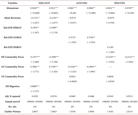
Table 1 below reports parameter coefficients and corresponding t-statistics from Equation (14), three models have been estimated using NZD/AUD, NZD/USD and AUD/USD exchange rates as dependent variables. Results are remarkably consistent across all currency pairs. First, the effects of momentum and com-modity prices movements are uniformly strong and consistent in all three spe-cific models. Second, majority of coefficients from respective regression models are in the theoretically correct sign and are statistically significant, with only two exceptions which is the US commodity price and the GDP change between US and New Zealand. Third, there is no evidence to support the significance of US commodity prices that could be related to the movements of either the NZD/USD or the AUD/USD exchange rate dynamics. Therefore, these results confirm the hypothesis that Australian and New Zealand commodity prices should be applied to measure the exchange rate movement. In addition, results indicate that when putting macroeconomic variables into the regression model, the NZD/AUD cross rate model does provide superior results than others.

DOI: 10.4236/***.2017.***** 12 Theoretical Economics Letters Table 1. Exchange Rates and Commodity Prices Dynamics: General to Specific Models. This table reports coefficients and t-statistics from Equation (14). We conduct both the “general” model (Columns 2, 4 and 6) and the ‘specific model (columns 3, 5 and 7). We eliminate variables that are insignificant from the “general” model until all remaining variables are significant in the “specific” model. The dependent variable is the actual exchange rates between NZD/AUD, AUD/USD and NZD/USD. The cor-responding t-statistics are reported in parentheses. All variables are in logarithm forms. We have included NZ Migration as an explanatory variable because of the general-to-specific search indicated that it is statistically significant. The relative GDP is lagged for three periods as GDP data is quarterly. *, ** and *** indicate statistical significant at the 10%, 5%, and 1% level, respectively.

Variables NZD/AUD AUD/USD NZD/USD

Momentum 0.9429*** 0.9521*** 0.9867*** 0.9849** 0.9822*** 0.9789***

(−55.809) (−56.805) −70.463 (−72.490) (−73.800) (−74.520)

Mean Reversion −0.1521** −0.1301** −0.0751 −0.0579

(−2.437) (−2.077) (−0.957) (−0.794)

Ral.GDP.NZ&AU 0.1876** 0.1890**

(−2.187) (−2.178)

Ral.GDP.AU&US 0.3733* 0.3749**

(−1.955) (−1.976)

Ral.GDP.NZ&US 0.1205

(−1.304)

NZ Commodity Prices −0.1977*** −0.2099*** −0.2192*** −0.2131***

(−3.560) (−3.748) (−3.923) (-4.583)

AU Commodity Prices 0.1906*** 0.1798*** −0.3326*** −0.2994*** −−

(−3.771) (−3.526) (−5.323) (−5.995)

US Commodity Prices 0.0423 0.0030

(−0.9828) (−0.078)

NZ Migration 0.0000***

(−2.727)

Adj. R-squared 0.9293 0.9276 0.9485 0.9486 0.9543 0.9515

Sample period 1986M1-2010M1 1986M1-2010M1 1986M1-2010M1 1986M1-2010M1 1986M1-2010M1 1986M1-2010M1

No. obs. 291 291 291 291 291 291

Durbin-Watson 2.0057 1.9823 1.9336 1.9903 1.9181 2.0135

DOI: 10.4236/***.2017.***** 13 Theoretical Economics Letters

possible explanation is that the flow of migrant funds may affect supply and de-mand of both currencies, hence the net effect of migration is expected to play an

active role in determining the cross-exchange rate dynamic12_{. Munroe [18]}

found that “migration flows (between New Zealand and Australia) have an out-sized effect on the housing market, which causes large flows of funds, and affect the exchange rate indirectly via interest rates”. Despite the fact that New Zealand net migration towards Australia is a statistically significant variable in the model, we excluded it from our further analysis as it is deemed to be economically in-significant because the coefficient is 0.0000019.

5.2. Regression Models with Structural Breaks

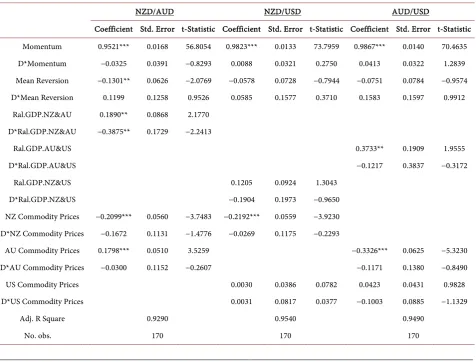
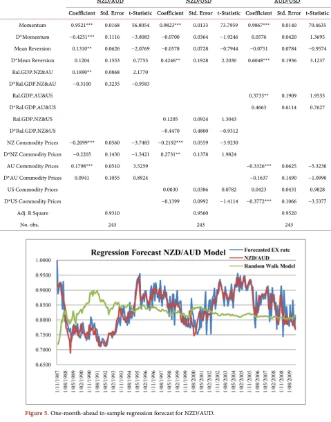
We now turn to examine possible structural breaks during our sample period. Two possible structural breaks are chosen to reflect two most recent major fi-nancial crises; early 2001 and late 2007. We simply give the time-dependent dummy variable a value of “one” for the period before the break date and a value of “zero” for the period after the break date. Results in Table 2 and Table 3 sug-gest that coefficients of time dependent variable provide relatively little evidence of any structural break. We therefore conclude that we may have some possible small parameter shifts for the sample period, and the expected sign and magni-tude of coefficients are stable over the entire sample period without systematic structural breaks. We now turn to explore in-sample and out-of-sample fore-casting performances for the NZD/AUD cross rate model.

5.3. In-Sample and Out-of-Sample Forecasting

In this section, the following regression equation is going to be used to perform the in-sample forecasting for NZD/AUD cross rate:

(

)

(

)

(

)

(

)

(

)

&

1 1 2 1 3 3

4 1 5 1

.

. .

NZ AU

t k t k t k t k

t k t k t k

Error Error Error Ral GDP

NZ ComPr AU ComPr

α β β β

β β ε

+ + − + − + −

+ − + − +

= + + ∆ + ∆

+ + + (15)

Figure 5 below presents the performance of the commodity-price-augmented regression model we developed for forecasting NZD/AUD cross exchange rate movements (Equation 15). It provides us a visual observation for the in-sample

NZD/AUD cross rate forecasting test14_{. We include results from a random walk}

model and the actual NZD/AUD cross market exchange rate. All parameters are estimated using data from January 1986 to January 2010. The movement of the blue-line (representing the in-sample one-month-ahead forecasted NZD/AUD cross exchange rates) is remarkably close to the red line (the actual NZD/AUD market cross exchange rate). This indicates an excellent in-sample forecasting of our NZD/AUD cross rate model. This model not only picks up every major 12_{According to Statistic NZ, the biggest destination for New Zealand emigrants is by far its best}

neighbor—Australia. Moreover, Australia is the second in line among the countries that listed as the biggest source of New Zealand’s immigrants with account for 20% of all migrant arrivals.

13_{See Appendix B for an illustration of the out-of-sample forecasting in details.}

14_{In-sample forecasting period is from the 1}st _{month of year 1986 to 1}st _{month of 2010, of which 219}

DOI: 10.4236/***.2017.***** 14 Theoretical Economics Letters

trends of the exchange rate movement in past two decades, but also accurately measures exchange rate turning point, represented by peaks and troughs in Fig-ure 5. Results from the Random Walk (RW) model (represented by the green line) show no signs of any predictability of actual NZD/AUD cross rates over the entire sample period. From early 1987 to the beginning of 1991, the Random Walk model completely mis-specified the underlying exchange rate movement. The Random Walk model also underestimates the volatility of NZD/AUD cross rate over time. It offers no prediction of the changes of direction on the currency movement after 1991.

However, despite the superiority of our NZD/AUD cross rate in-sample fore-casting model, it is necessary for us to use contemporaneous data when con-ducting such estimates. Therefore, an out-of-sample forecast performance test is to be conducted. For out-of-sample forecasting, we first adopt standard quantit-ative procedures involved in forecasting the departure from the fair value from

Equation (12), where the forecasting errors are defined as: FEt k+ =St k+ −St k+ ,

where k≥1 _and S_{t k}+ represents the k-step-ahead forecast.

We measure forecasting errors for four time intervals, 1-month-ahead,

Table 2. OLS with Possible Structural Break. This table provides the regression results for possible structural breaks with the break point set at January 2001. This break point is selected as at the first month of year 2001 to reflect the most recent major global financial crisis. *, **, and *** indicate significance at the 10%, 5%, and 1% levels, respectively.

NZD/AUD NZD/USD AUD/USD

Coefficient Std. Error t-Statistic Coefficient Std. Error t-Statistic Coefficient Std. Error t-Statistic

Momentum 0.9521*** 0.0168 56.8054 0.9823*** 0.0133 73.7959 0.9867*** 0.0140 70.4635

D*Momentum −0.0325 0.0391 −0.8293 0.0088 0.0321 0.2750 0.0413 0.0322 1.2839

Mean Reversion −0.1301** 0.0626 −2.0769 −0.0578 0.0728 −0.7944 −0.0751 0.0784 −0.9574

D*Mean Reversion 0.1199 0.1258 0.9526 0.0585 0.1577 0.3710 0.1583 0.1597 0.9912

Ral.GDP.NZ&AU 0.1890** 0.0868 2.1770

D*Ral.GDP.NZ&AU −0.3875** 0.1729 −2.2413

Ral.GDP.AU&US 0.3733** 0.1909 1.9555

D*Ral.GDP.AU&US −0.1217 0.3837 −0.3172

Ral.GDP.NZ&US 0.1205 0.0924 1.3043

D*Ral.GDP.NZ&US −0.1904 0.1973 −0.9650

NZ Commodity Prices −0.2099*** 0.0560 −3.7483 −0.2192*** 0.0559 −3.9230

D*NZ Commodity Prices −0.1672 0.1131 −1.4776 −0.0269 0.1175 −0.2293

AU Commodity Prices 0.1798*** 0.0510 3.5259 −0.3326*** 0.0625 −5.3230

D*AU Commodity Prices −0.0300 0.1152 −0.2607 −0.1171 0.1380 −0.8490

US Commodity Prices 0.0030 0.0386 0.0782 0.0423 0.0431 0.9828

D*US Commodity Prices 0.0031 0.0817 0.0377 −0.1003 0.0885 −1.1329

Adj. R Square 0.9290 0.9540 0.9490

DOI: 10.4236/***.2017.***** 15 Theoretical Economics Letters Table 3. OLS with Possible Structural Break. This table provides the regression results for possible structural breaks with the break point set at December 2007. This break point is selected as at the last month of year 2007 to reflect the most recent major global financial crisis. *, **, and *** indicate significance at the 10%, 5%, and 1% levels, respectively.

NZD/AUD NZD/USD AUD/USD

Coefficient Std. Error t-Statistic Coefficient Std. Error t-Statistic Coefficient Std. Error t-Statistic

Momentum 0.9521*** 0.0168 56.8054 0.9823*** 0.0133 73.7959 0.9867*** 0.0140 70.4635

D*Momentum −0.4251*** 0.1116 −3.8083 −0.0700 0.0364 −1.9246 0.0576 0.0420 1.3695

Mean Reversion 0.1310** 0.0626 −2.0769 −0.0578 0.0728 −0.7944 −0.0751 0.0784 −0.9574

D*Mean Reversion 0.1204 0.1553 0.7753 0.4246** 0.1928 2.2030 0.6048*** 0.1936 3.1237

Ral.GDP.NZ&AU 0.1890** 0.0868 2.1770

D*Ral.GDP.NZ&AU −0.3100 0.3235 −0.9583

Ral.GDP.AU&US 0.3733** 0.1909 1.9555

D*Ral.GDP.AU&US 0.4663 0.6114 0.7627

Ral.GDP.NZ&US 0.1205 0.0924 1.3043

D*Ral.GDP.NZ&US −0.4470 0.4800 −0.9312

NZ Commodity Prices −0.2099*** 0.0560 −3.7483 −0.2192*** 0.0559 −3.9230

D*NZ Commodity Prices −0.2205 0.1430 −1.5421 0.2731** 0.1378 1.9824

AU Commodity Prices 0.1798*** 0.0510 3.5259 −0.3326*** 0.0625 −5.3230

D*AU Commodity Prices 0.0941 0.1055 0.8924 −0.1637 0.1490 −1.0990

US Commodity Prices 0.0030 0.0386 0.0782 0.0423 0.0431 0.9828

D*US Commodity Prices −0.1399 0.0992 −1.4114 −0.3772*** 0.1066 −3.5377

Adj. R Square 0.9310 0.9560 0.9520

No. obs. 243 243 243

DOI: 10.4236/***.2017.***** 16 Theoretical Economics Letters

3-month-ahead, 6-month-ahead and 12-month-ahead. The estimation involves the prediction of the long term Fair Value (FV) of NZD/AUD cross rate, this FV is not constant over time. We first need to define the FV before the forecasting error can be derived. To ensure a theoretically sound process of approximating FVs, we apply four methods to predict FVs over the testing time horizon. Firstly, we assume the Fair Value (FV) is known for the out-of-sample period. Hence, FVs are directly taken from the in-sample forecasting models which have been

done in the previous section15_{. Secondly, FVs are assumed to be unknown for the}

out-of-sample period, and are therefore predicted using an AR(1) model, an ARMA(1, 1) model and a random walk model, respectively. To evaluate the fo-recasting performance, four fofo-recasting measures are applied: Root Mean Square Error (RMSE), Mean Absolute Error (MAE), Mean Absolute Percentage Error (MAPE) and Theil Inequality Coefficient (THEIL).

These measurements offer a set of quantitative values, which specifically measure how far the forecasted fair values are away from the actual observed exchange rates. A lower value indicates a better fit, hence, higher accuracy of the forecasting model. The out-of-sample forecasting involves re-estimating the NZD/AUD cross rate for each historical period, using only data that would have been available to us at that time. Appendix B provides a detailed illustration for a 3-month-ahead out-of-sample forecasting.

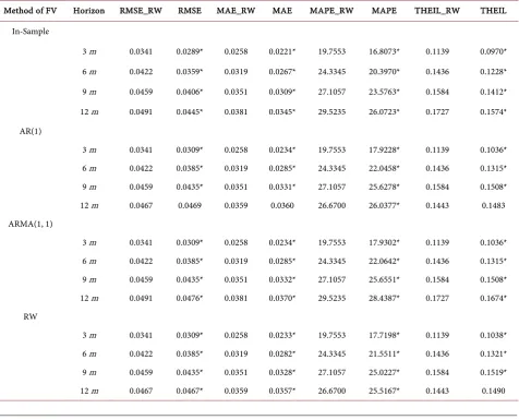
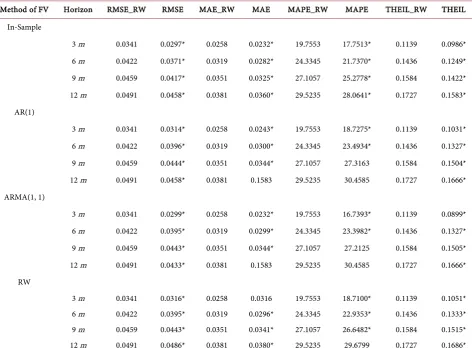
Table 4 and Table 5 present forecasting errors for the out-of-sample perfor-mance. Results suggest that our commodity price augmented forecasting model remarkably beat the random walk model in every setting under 3- and 6-month testing periods. For 9- and 12-month period, results also suggest that forecasting errors are constantly smaller in most cases. This indicates that our NZD/AUD cross exchange rate forecasting model outperforms the random walk model in majority of the testing time periods. It is necessary to mention that the Random Walk model has been widely considered as the benchmark for exchange rate fo-recasting models. Based on existing literatures, the Random Walk model works superior compared to other forecasting models. We pick up two sample starting points when conducting out-of-sample forecasting performances: (1) February 1990; and (2) March 1993. These starting points are chosen for the following reasons: New Zealand and Australia both adopted inflation-targeting monetary

policyfor period between 1990 and 1993. Therefore, it is theoretically sound for

future exchange rate forecasting to use the data set available before and after the exchange rate regime shift. In addition to the exchange rate regime shift, the out-of-sample period also spans a period of sharp exchange rate depreciation as well as the sustained appreciation, which began in 1992. Thus, our exchange rate model is believed to better facilitate a more comprehensive model evaluation across the out-of-sample forecasting period. Contrary to previous findings, our fundamental macroeconomic variable exchange rate model has a better fore-casting accuracy in short-time horizons (3-month and 6-month) relative to

15_{The in-sample forecasting period is from the 1}st _{month of year 1986 to 1}st _{month of 2010, which}

DOI: 10.4236/***.2017.***** 17 Theoretical Economics Letters

longer time horizons (9-month and 12-month).

6. Conclusion

The relationship between the exchange rate and fundamental macroeconomic variables has drawn lots of attentions to many researchers for many years, yet, no clear consensus has been emerged. In this paper, we focus on a set of selective currencies which are considered as the “Commodity Currencies”, namely the New Zealand and the Australian dollars. We incorporate commodity prices from these two countries into the exchange rate forecasting model. Results shed extra light on two main issues. Firstly, commodity currencies are not the same across

countries. Some are more of “commodity currencies” than others, i.e. more

pro-nounce in New Zealand and Australia than in the U.S. This is due to the fact that

Table 4. Out-of-Sample Forecasting (from Mar. 1993). This table reports Out-of-Sample forecasting performance compared to the Random Walk model. The sample period starts from March 1993 to May 2002, and forecasting period is from May 2002 to January 2010. The evaluation results of RW model are reported in columns 3, 5, 7 and 9 and the ‘built in’ models (Equation (15)) are reported in columns 4, 6, 8 and 10. Root Mean Square Error (RMSE), Mean Absolute Error (MAE), Mean Absolute Percentage Error (MAPE) and Theil Inequality Coefficient (THEIL) offer a set of quantitative values, which specifically measure how far away the model forecasted exchange rates are to the actual exchange rates observed later. A lower value indicates a better fit (higher accuracy) of the tested model. * indicates forecasting superiority over RW model.

Method of FV Horizon RMSE_RW RMSE MAE_RW MAE MAPE_RW MAPE THEIL_RW THEIL

In-Sample

3 m 0.0341 0.0289* 0.0258 0.0221* 19.7553 16.8073* 0.1139 0.0970*

6 m 0.0422 0.0359* 0.0319 0.0267* 24.3345 20.3970* 0.1436 0.1228*

9 m 0.0459 0.0406* 0.0351 0.0309* 27.1057 23.5763* 0.1584 0.1412*

12 m 0.0491 0.0445* 0.0381 0.0345* 29.5235 26.0723* 0.1727 0.1574*

AR(1)

3 m 0.0341 0.0309* 0.0258 0.0234* 19.7553 17.9228* 0.1139 0.1036*

6 m 0.0422 0.0385* 0.0319 0.0285* 24.3345 22.0458* 0.1436 0.1315*

9 m 0.0459 0.0435* 0.0351 0.0331* 27.1057 25.6278* 0.1584 0.1508*

12 m 0.0467 0.0469 0.0359 0.0360 26.6700 26.0377* 0.1443 0.1483

ARMA(1, 1)

3 m 0.0341 0.0309* 0.0258 0.0234* 19.7553 17.9302* 0.1139 0.1036*

6 m 0.0422 0.0385* 0.0319 0.0285* 24.3345 22.0642* 0.1436 0.1315*

9 m 0.0459 0.0435* 0.0351 0.0332* 27.1057 25.6551* 0.1584 0.1508*

12 m 0.0491 0.0476* 0.0381 0.0370* 29.5235 28.4387* 0.1727 0.1674*

RW

3 m 0.0341 0.0309* 0.0258 0.0233* 19.7553 17.7198* 0.1139 0.1038*

6 m 0.0422 0.0385* 0.0319 0.0282* 24.3345 21.5511* 0.1436 0.1321*

9 m 0.0459 0.0435* 0.0351 0.0328* 27.1057 25.0227* 0.1584 0.1519*

DOI: 10.4236/***.2017.***** 18 Theoretical Economics Letters Table 5. Out-of-Sample Forecasting (from Feb. 1990). This table reports Out-of-Sample forecasting performance compared to the Random Walk model. The sample period starts from Feb. 1990 to May 2002, and forecasting period is from May 2002 to January 2010. The evaluation results of RW model are reported in columns 3, 5, 7 and 9 and the “built in” models (Equation (15)) are re-ported in columns 4, 6, 8 and 10. Root Mean Square Error (RMSE), Mean Absolute Error (MAE), Mean Absolute Percentage Er-ror (MAPE) and Theil Inequality Coefficient (THEIL) offer a set of quantitative values, which specifically measure how far away the model forecasted exchange rates are to the actual exchange rates observed later. A lower value indicates a better fit (higher accuracy) of the tested model. * indicates forecasting superiority over RW model.

Method of FV Horizon RMSE_RW RMSE MAE_RW MAE MAPE_RW MAPE THEIL_RW THEIL

In-Sample

3 m 0.0341 0.0297* 0.0258 0.0232* 19.7553 17.7513* 0.1139 0.0986*

6 m 0.0422 0.0371* 0.0319 0.0282* 24.3345 21.7370* 0.1436 0.1249*

9 m 0.0459 0.0417* 0.0351 0.0325* 27.1057 25.2778* 0.1584 0.1422*

12 m 0.0491 0.0458* 0.0381 0.0360* 29.5235 28.0641* 0.1727 0.1583*

AR(1)

3 m 0.0341 0.0314* 0.0258 0.0243* 19.7553 18.7275* 0.1139 0.1031*

6 m 0.0422 0.0396* 0.0319 0.0300* 24.3345 23.4934* 0.1436 0.1327*

9 m 0.0459 0.0444* 0.0351 0.0344* 27.1057 27.3163 0.1584 0.1504*

12 m 0.0491 0.0458* 0.0381 0.1583 29.5235 30.4585 0.1727 0.1666*

ARMA(1, 1)

3 m 0.0341 0.0299* 0.0258 0.0232* 19.7553 16.7393* 0.1139 0.0899*

6 m 0.0422 0.0395* 0.0319 0.0299* 24.3345 23.3982* 0.1436 0.1327*

9 m 0.0459 0.0443* 0.0351 0.0344* 27.1057 27.2125 0.1584 0.1505*

12 m 0.0491 0.0433* 0.0381 0.1583 29.5235 30.4585 0.1727 0.1666*

RW

3 m 0.0341 0.0316* 0.0258 0.0316 19.7553 18.7100* 0.1139 0.1051*

6 m 0.0422 0.0395* 0.0319 0.0296* 24.3345 22.9353* 0.1436 0.1333*

9 m 0.0459 0.0443* 0.0351 0.0341* 27.1057 26.6482* 0.1584 0.1515*

12 m 0.0491 0.0486* 0.0381 0.0380* 29.5235 29.6799 0.1727 0.1686*

Australia and New Zealand are commodity-export dependent countries. They

also share some distinctive economic structures and policies, comparing to other

countries. In this regard, considerations should not be solely given to commod-ity export components, but various other factors as well. Results in our study confirmed that there is a strong and robust relationship between the exchange rate and commodity prices in Australia and New Zealand.

consistent-DOI: 10.4236/***.2017.***** 19 Theoretical Economics Letters

ly outperforms a random walk at short horizons according to four evaluating methods. However, there are some evidences suggest that, in out-of-sample forecasts, the superiority of such a model does slightly deteriorate as the fore-casting horizon increases.

The attributes behind our empirical results are likely to be the “Enhanced Commodity Currencies Phenomenon”, represented by the fact that both under-lying currencies (NZD and AUD) are commodity currencies, and they are both subject to the “Commodity Currencies Phenomenon” discovered in recent lit-eratures. In addition, there is a unique underlying economic relationship be-tween these two OECD nations: close geographically, free from trade

restric-tions, high co-movement in financial markets, are contributing to our

findings.

Results in this paper have provided further understanding of exchange rate dynamics to commodity prices. In addition, the superior and potential exploit-able forecast ability of commodity-price-augmented exchange rate forecasting model may provide important information for nations that heavily rely on pri-mary commodity production, and wish to develop the capital market liberaliza-tion by moving towards floating exchange rate regimes. The model developed in this paper can also benefit portfolio managers in better modeling NZD/AUD cross rates, hence, making better strategic decisions on currency trading and portfolio rebalancing.

References

[1] Meese, R.A. and Rogoff, K. (1983) Empirical Exchange Rate Models of the Seven-ties: Do They Fit out of Sample? Journal of International Economics, 14, 3-24. [2] Meese, R.A. and Rogoff, K. (1983) The Out-of-Sample Failure of Empirical

Ex-change Rate Models. In: Frenkel, J.A., Ed., Exchange Rates and International

Mac-roeconomics, University of Chicago Press, Chicago, 67-112.

[3] Mussa, M. (1979) Empirical Regularities in the Behavior of Exchange Rates and Theories of the Foreign Exchange Market. In: Brunner, K. and Meltzer, A.H., Eds.,

Policies for Employment, Prices, and Exchange Rates, North-Holland Pub. Co.,

New York, 9-57.

[4] Calvo, G. and Rodriguez, C. (1977) A Model of Exchange Rate Determination under Currency Substitution and Rational Expectations. Journal of Political Economy, 85, 617-626.https://doi.org/10.1086/260586

[5] Stockman, A.C. (1980) A Theory of Exchange Rate Determination. Journal of

Po-litical Economy, 88, 673-698.https://doi.org/10.1086/260897

[6] Lucas, R. (1982) Interest Rates and Currency Prices in a Two-Country World.

Journal of Monetary Economics, 10, 335-359.

[7] Cashin, P., Cespedes, L. and Sahay, R. (2004) Commodity Currencies and the Real Exchange Rate. Journal of Development Economics, 75, 239-268.

[8] Chen, Y. and Rogoff, K. (2003) Commodity Currencies. Journal of International

Economics, 60, 133-160.

DOI: 10.4236/***.2017.***** 20 Theoretical Economics Letters [10] Chen, Y. (2004) Exchange Rates and Fundamentals: Evidence from Commodity

Economies. University of Washington, Working Paper.

[11] Chen, Y. and Rogoff, K. (2006) Are the Commodity Currencies an Exception to the Rule? University of Washington, Working Paper.

[12] Amano, R. and Norden, S. (1995) A Forecasting Equation for the Canada—U.S. Dollar Exchange Rate. The Exchange Rate and the Economy (207-65), Bank of Canada, Ottawa.

[13] Gruen, D.R. and Wilkinson, J. (1994) Australia’s Real Exchange Rate—Is It Ex-plained by the Terms of Trade or by Real Interest Differentials? Economic Record, 70, 204-219.https://doi.org/10.1111/j.1475-4932.1994.tb01839.x

[14] De Gregorio, J. and Wolf, H.C. (1994) Terms of Trade, Productivity, and the Real Exchange Rate (Working Papers 94-19). New York University.

[15] Chinn, M. and Johnston, L. (1996) Real Exchange Rate Levels, Productivity and Demand Shocks: Evidence from a Panel of 14 Countries. Working Paper 5709, NBER.

[16] Montiel, P.J. (1997) Exchange Rate Policy and Macroeconomic Management in ASEAN Countries. In: Hinklin, J., Robinson, D. and Singh, A., Eds.,

Macroeco-nomic Issues Facing ASEAN Countries, International Monetary Fund, Washington

DC, 253-298.

[17] Chen, Y., Rogoff, K. and Rossi, B. (2008) Can Exchange Rates Forecast Commodity Prices? Working Paper 13901, NBER.

[18] Munroe, A. (2004) What Drives the New Zealand Dollar. Reserve Bank of New

DOI: 10.4236/***.2017.***** 21 Theoretical Economics Letters

Appendix A

CBA NZ Commodity Price Index (base at 01/01/1986 = 100)

The Commonwealth Bank New Zealand Commodity Price Index is based on 18 different commodities that make up over 60% of New Zealand’s total mer-chandise exports. The index includes: the major forestry products (logs, pulp, paper); dairy products (e.g. whole & skim milk powder, butter, cheese, and casein); other livestock products (e.g. wool, lamb, & beef, leather and skins); as-sorted commodities such as aluminium, fruit, fish, and crude petroleum prod-ucts. The commodity weights are determined by the importance of each

com-modity in New Zealand’s trade, i.e. Dairy 35%, Forestry 20%, Livestock 30%,

Fi-shery 8%, Aluminum 7%. For example, in 2010 the CBA NZ Commodity Price Index weights are based on contributions to merchandise exports in the previous year (2009). The weights for 2010 are: Wool 0.033; Beef 0.093; Lamb 0.150; Venison 0.013; Skins 0.019; Dairy 0.383; Apples 0.021; Kiwifruit 0.053; Logs 0.049; Sawn Timber 0.045; Wood Pulp 0.030; Seafood 0.065; Aluminium 0.046.

RBA Commodity Index SDR (Index of Commodity Prices)

The ICP is a Laspeyres index, which means that the index is a weighted aver-age of recent changes in commodity prices. While the initial weight given to each commodity reflects its relative importance in total commodity export earnings in the base period, at any point in time thereafter the effective weight of each commodity in the index reflects the impact of subsequent changes in its price. However, since export values change as a result of movements in quantities ex-ported as well as changes in prices, it is necessary to update periodically the base-period weights to reflect changes in export volumes. In addition, since the importance of individual commodities in Australia’s export values changes over time—with the weight of some commodities becoming very small while others rise in importance—it is necessary to periodically review the commodities that are included in the index. RBA staffs have recently completed such a review, with up-dating conducted in 2003. As a result, the following changes have been made:

• _{the ICP will be re-based from 2001/02 to 2008/09;}

• crude oil will be reintroduced to the index and the whole history of the ICP

back-cast accordingly; and

• milk powder will be added and rice will be excluded from the index,

back-cast to July 2008.

The updated index will include the prices of 20 of Australia’s key commodity exports, which currently account for around 85 per cent of primary commodity export earnings. The re-basing to 2008/09 and addition of crude oil have a noti-ceable effect on the weights of each sub-index and individual commodity; adding milk powder and excluding rice have only small effects on the ICP.

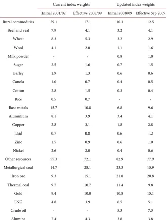
The following table shows the weights of each component in the RBA Com-modity Index SDR.

USA S&P GSCI Non-Energy Spot—Price Index

DOI: 10.4236/***.2017.***** 22 Theoretical Economics Letters Table A1. Commodity Price Weights (in %).

Current index weights Updated index weights

Initial 2001/02 Effective 2008/09 Initial 2008/09 Effective Sep 2009

Rural commodities 29.1 17.1 10.3 12.5

Beef and veal 7.9 4.1 3.2 4.1

Wheat 8.3 5.3 3.2 2.9

Wool 4.1 2.0 1.1 1.6

Milk powder - - 0.8 1.0

Sugar 2.5 1.6 0.7 1.5

Barley 1.9 1.3 0.6 0.6

Canola 1.0 0.7 0.4 0.5

Cotton 2.8 1.5 0.3 0.4

Rice 0.5 0.7 - -

Base metals 15.7 10.8 6.8 9.6

Aluminium 8.1 3.9 3.4 4.1

Copper 2.8 3.1 1.8 2.8

Lead 0.7 0.8 0.6 1.2

Zinc 1.5 0.9 0.6 1.0

Nickel 2.6 2.0 0.4 0.6

Other resources 55.3 72.1 82.9 77.9

Metallurgical coal 14.7 28.1 23.3 15.9

Iron ore 9.3 15.1 21.8 20.8

Thermal coal 9.7 10.7 11.4 9.8

Gold 9.4 10.0 10.8 15.1

LNG 4.8 3.9 6.5 5.1

Crude oil - - 5.3 7.3

Alumina 7.4 4.3 3.8 3.8

in the index is determined by the average quantity of production in the last five years of available data. Such weighting provides the S&P GSCI with significant advantages, both as an economic indicator and as a measure of investment per-formance. Below is a table from Goldman Sachs shown the most recent S&P GSCI index components and weight. For more detail about this index, readers can refer to following web address:

http://www2.goldmansachs.com/services/securities/products/sp-gsci-commodity -index/tables.html

S & P GSCI™ Components and Weights

DOI: 10.4236/***.2017.***** 23 Theoretical Economics Letters Table A2. AS&P GSCI™ Components and Dollar Weights (%) (October 6, 2010).

Energy 68.3 Industrial

8.57 Precious 3.56 Agriculture 15.18 Livestock 4.39

Crude Oil 35.65 Metals Metals Wheat 3.53 Live Cattle 2.57

Brent Crude Oil 14.58 Aluminium 2.6 Gold 3.13 Red Wheat 0.73 Cattle 0.42

RBOB Gas 4.3 Copper 3.88 Silver 0.42 Corn 3.8 Lean Hogs 1.4

Heating Oil 4.66 Lead 0.49 Soybeans 2.29

Gas Oil 5.92 Ni

0.92 Cotton 1.4

Natural Gas 3.21 Kel Sugar 2.29

Zinc 0.69 Coffee 0.85

Cocoa 0.31

Appendix B

An out-of-sample forecasting example: 3-month-ahead forecast

First, as we mentioned in the in-sample forecasting section, our sample period of in-sample forecasting is the full data set from January 1986 to January 2010. However, due to the consideration of the exchange rate regime shift, we define out-of-sample forecasting period as from February 1990/March 1993 to January 2010. We set May 2002 as time “t”, we assume it is the last month of the “in-sample” period and it is 3-month before the “out-of-sample” forecasting pe-riod. Next, we derive NZD/AUD long term fair value by adopting either one of the four methods we mentioned in the paper. Here, for simplicity, we assume FVs are all known and same as the FV values estimated in the in-sample fore-casting. Having the FVs, we can then generate a series of values termed “depar-tures from NZD/AUD Fair Value” by subtract the actual NZD/AUD exchange rates from corresponding FVs. This will give us 148 observations (from February 1990 to May 2002). We then perform the following regression for the departure from NZD/AUD cross rate fair value on independent variables:

(

)

(

)

(

)

(

)

(

)

&

1 1 2 1 3 4

4 1 5 1

.

. ( .

NZ AU

t k t k t k t k

t k t k t k

Error Error Error Ral GDP

NZ ComPr AU ComPr

α β β β

β β ε

+ + − + − + −

+ − + − +

= + + ∆ + ∆

+ + +

We then use corresponding parameters from above regression model to fore-cast the departure value of 3 month-ahead. And the forefore-casted departure is added to the corresponding FV value to derive the “3 month-ahead-forecasted

exchange rate”. Hence, the forecasting error at time t+3 is: FEt+3=St+3−St+3,

where St+3 represents the 3-month-ahead forecast. To do the out-of-sample

forecast of further 3 month-ahead NZD/AUD exchange rate from time “t + 3”,

the same process is repeated, but with 3 more set of observations added into the

initial 148 observations as they become available at time “t + 3”.

DOI: 10.4236/***.2017.***** 24 Theoretical Economics Letters Table A3. OLS tests of possible structure break.

NZD/AUD NZD/USD AUD/USD

OLS Test OLS + Break dummy OLS Test OLS + Break dummy OLS Test OLS + Break dummy

Momentum 0.952 *** 0.962 *** 0.965 *** 0.982 *** 0.996 *** 0.976 *** 0.987 *** 0.983 *** 0.957 ***

(56.805) (57.909) (44.763) (73.795) (66.960) (34.829) 70.46345 65.06186 35.41659

Mean Reversion −0.130 ** −0.127 * −0.204 ** −0.058 −0.177 ** −0.113 −0.075 −0.190 ** −0.140

(−2.077) (−1.848) (−2.364) (−0.794) (−2.043) (−0.895) −0.95738 −2.16437 −1.22082

Ral.GDP.NZ&AU 0.189 ** 0.221 ** 0.365 ***

(2.177) (2.492) (2.982)

Ral.GDP.AU&NZ 0.373 * 0.303 0.449 *

(1.955) (1.544) (1.615)

Ral.GDP.NZ&US 0.120 0.161 * 0.188 *

(1.304) (1.722) (1.615)

NZ Commodity Prices −0.210 *** −0.208 *** −0.118 −0.219 *** −0.289 *** −0.209 **

(−3.748) (−3.312 (−1.381) (−3.922) (−4.516） (−2.257)

AU Commodity Prices 0.179824 *** −0.1846 *** 0.228426 ** −0.33262 *** −0.29504 *** −0.23721 **

(3.526) (2.782) (2.341) (−5.323) (−3.879) (−2.071)

US Commodity Prices 0.003 0.019 0.004 0.042 0.089 * 0.086

(−0.078) (0.416) (0.059) (0.982) (1.816) (1.288)

Breakpoint 2007M12 2000M1 2007M12 2000M1 2007M12 2000M1

Adj.R^2 0.928 0.931 0.929 0.954 0.956 0.954 0.948 0.952 0.949

No. obs. 268 243 170 268 243 170 268 243 170

Sample period 1986M1-2010M1

This table reports the original OLS regression results as well as the OLS results

after each breaking point is added into the regression models, where βt = 1 if t ≥

1 Breakpoint and βt = 0 otherwise. Breakpoints are selected as the starting of the

Massey Documents by Type Journal Articles

The commodity price and exchange rate dynamics

Zou, L

2017-10-02