The many lives of active galactic nuclei II: the formation and evolution of radio jets and their impact on galaxy evolution

The many lives of active galactic nuclei–II: The formation and evolution

of radio jets and their impact on galaxy evolution

Mojtaba Raouf,

Stanislav S. Shabala,

Darren J. Croton,

Habib G. Khosroshahi

and Maksym Bernyk

1_{School of Astronomy, Institute for Research in Fundamental Sciences (IPM), Tehran 19395–5531, Iran}

2_{Centre for Astrophysics and Supercomputing, Swinburne University of Technology, PO Box 218 Hawthorn, Victoria 3122, Australia} 3_{School of Physical Sciences, Private Bag 37, University of Tasmania, Hobart TAS 7001, Australia}

Accepted 2017 June 22. Received 2017 June 20; in original form 2016 November 16

A B S T R A C T

We describe new efforts to model radio active galactic nuclei (AGN) in a cosmological context using the Semi-Analytic Galaxy Evolution (SAGE) semi-analytic galaxy model. Our new method tracks the physical properties of radio jets in massive galaxies including the evolution of radio lobes and their impact on the surrounding gas. This model also self consistently follows the gas cooling–heating cycle that significantly shapes star formation and the life and death of many galaxy types. Adding jet physics to SAGE adds new physical properties to the model output, which in turn allows us to make more detailed predictions for the radio AGN population. After calibrating the model to a set of core observations we analyse predictions for jet power, radio cocoon size, radio luminosity and stellar mass. We find that the model is able to match the stellar mass-radio luminosity relation atz∼0 and the radio luminosity function out toz∼1. This updated model will make possible the construction of customised AGN-focused mock survey catalogues to be used for large-scale observing programs.

Key words: methods: numerical – galaxies: active – galaxies: evolution – galaxies: haloes – galaxies: jets.

1 I N T R O D U C T I O N

The paradigm of hierarchical galaxy formation provides a re-markably successful framework to explain many properties of the observed galaxy population, particularly at intermediate masses (Press & Schechter1974; White & Rees1978; White & Frenk1991; Lacey & Cole 1994). With early models over-predicting galaxy counts at both the bright and faint end of the luminosity function, it was quickly realized how important feedback processes were for reproducing the observations. At the low mass end, heating due to the reionization of the Universe at early times, and supernovae ejecta from the most massive stars, became critical to explain the deficit of faint galaxies with respect to the number of low mass haloes (Efstathiou1992). However in the most massive haloes such feedback modes proved insufficient to offset rapid cooling of the hot gas, leading to a subsequent overproduction of massive ellip-tical galaxies by many orders of magnitude.1_{Furthermore, optical}

_{E-mail:[email protected]}

1_{The ratio of galaxy stellar mass to dark matter halo mass decreases with}

increasing mass. Hence, even at a constant specific star formation rate the efficiency with which supernova can eject gas out of the gravitational poten-tial decreases with mass. In reality, massive ellipticals have lower specific

observations showed these massive ellipticals to have formed only a small fraction of their stars over the last half of the Hubble time (Bender & Saglia1999), in sharp contrast to the models which predicted that these objects should be rapidly forming stars at the present epoch.

A closely related problem was presented by galaxy clusters. Ob-servations of X-ray emission suggested that there should be runaway cooling of the hot (∼107_{K) gas (the so-called ‘cooling catastrophe’;}

Cowie & Binney1977; Fabian & Nulsen1977), however no such rapidly cooling gas at temperatures below about a third of the virial temperature was found (Tamura et al.2001; Peterson et al.2003). A new mechanism was required to offset gas cooling on scales of tens of kpc, and suppress excessive galaxy growth from star formation.

Silk & Rees (1998) pointed out that the presence of a super-massive black hole (SMBH) at the centre of every super-massive galaxy provides such a mechanism, through conversion of a fraction of accreted mass to thermal or kinetic energy (Penrose & Floyd1971; Blandford & Znajek1977; Blandford & Payne1982); this is the mechanism invoked to explain the presence of active galactic nuclei (AGN). By coupling a fraction of the AGN energy output to the

star formation rates than spirals, and the impact of the supernova is even smaller.

rapidly cooling hot halo gas, a new generation of galaxy formation models (Granato et al.2004; Bower et al.2006; Croton et al.2006; Monaco et al.2006) succeeded in reproducing the quenching of late epoch star formation in the most massive galaxies. While suc-cessful in the sense of reproducing the observed galaxy properties, these models do not make detailed predictions for the mechanisms through which AGN energy couples to the gas.

Broadly speaking, AGN feedback can be either mechanical (through radio jets) or radiative (see reviews by Cattaneo et al.2009; Somerville & Dav´e2015), with radiative feedback affecting the in-terstellar medium of the host galaxy, and radio jets doing feedback on the larger halo scales. For this reason, Croton et al. (2006) re-ferred to the mode of AGN feedback responsible for suppressing star formation sincez∼1 as ‘radio’ or ‘maintenance’ mode feed-back. Dramatic evidence for this mode of feedback in action was found in the Perseus (B¨ohringer et al.1991; Fabian et al.2003) and Virgo (Churazov et al.2001; Forman et al.2005) clusters, where lobes of radio emitting plasma were observed to displace the X-ray emitting gas away from the rapidly cooling central regions.

Observationally, the radio loud AGN fraction is found to be a strong function of host galaxy properties: Sadler, Jenkins & Kotanyi (1989) found more than 40 per cent of massive ellipticals to host low-luminosity radio sources. Best et al. (2005) showed that this fraction scales strongly with stellar mass, and this scaling is con-sistent with a picture of ‘maintenance mode’ feedback, in which massive galaxies with rapidly cooling hot haloes are more likely to host AGN, which can in turn provide the feedback needed to offset the otherwise imminent cooling catastrophe. In clusters, the state of the cooling gas appears to be intimately connected to the probability of finding an AGN in the cooling gas: Burns (1990) reported that over 70 per cent of cool core clusters hosted radio sources, com-pared to only 23 per cent of non-cool core clusters. Other authors (e.g. Mittal et al.2011) have found similar results.

While many of these sources are compact (Shabala et al.2008; Sadler et al.2014), when the jets are powerful enough they can break through the galaxy disc and inflate pairs of lobes of radio emitting synchrotron plasma, with the largest lobes up to a Mpc in size (Laing, Riley & Longair1983; Saripalli et al.1986, see Banfield et al.2016for an example of a recent discovery). Mor-phologically, extended radio lobes are observed to be either core or edge-brightened; such sources are classified as Fanaroff–Riley type I and type II, respectively (Fanaroff & Riley1974).

Large radio sources can do feedback well outside the host galaxy disc via two channels. First, powerful radio sources can drive strong shocks through the surrounding gas (Schoenmakers et al. 2000; Rawlings & Jarvis2004; Shabala, Kaviraj & Silk2011), heating and uplifting it to large radii. Secondly, lower power sources in galaxy clusters are often observed to give rise to buoyant bubbles of radio plasma, which displace the hot X-ray emitting gas as they rise through the cluster (B¨ohringer et al.1991; Churazov et al.2001; Fabian et al.2003; Forman et al.2005).

Multiple lines of evidence suggest that radio AGN activity must be episodic. Theoretically, AGN intermittency is expected in a self-regulating feedback process (e.g. Bahcall et al.1997; Kawata & Gibson2005; Novak, Ostriker & Ciotti2011; Gaspari, Brighenti & Temi2015). Observationally, the presence of multiple shocks and ripples around the X-ray cavities in the Perseus (Fabian et al.2003) and Virgo (Forman et al.2005) clusters have been interpreted as remnants of multiple AGN outbursts. Perhaps the most dramatic evidence for recurrent radio AGN activity is provided by sources with multiple pairs of radio lobes (e.g. Schoenmakers et al.2000). In these ‘double–double’ radio sources, the inner pair of lobes is

interpreted to correspond to the most recent AGN outburst, while the outer pair of lobes is due to a previous episode of AGN activ-ity. In a number of sources (e.g. Centaurus A; Israel1998; Feain et al.2009, a similar suggestion has also been made for Cygnus A, Chon et al.2012), the jet directions are often misaligned between outbursts, providing a mechanism for isotropizing the coupling of jet energy to cluster gas.

The interaction between radio jets/lobes and the hot atmospheres into which they expand sets both the properties of the observed AGN, such as their sizes, morphologies, luminosities and radio spectra; and through feedback, those of their host galaxies. The ef-fect of environment on both AGN properties and the amount of feed-back they do has been extensively studied through radio source dy-namical models (Scheuer1974; Begelman & Cioffi1989; Kaiser & Alexander1997; Alexander2002; Shabala et al.2008; Turner & Shabala2015), and numerical simulations (Norman et al.1982; Reynolds, Heinz & Begelman 2002; Basson & Alexander2003; Krause 2005; Mendygral, Jones & Dolag 2012; Hardcastle & Krause2013,2014). Recently, Godfrey & Shabala (2016) pointed out that the often quoted relationship between jet kinetic power and radio luminosity (derived from observations of X-ray deficient cavities, e.g. Birzan et al. 2004, 2008; Cavagnolo et al. 2010) is in fact driven by strong selection effects, and the true rela-tionship is more complicated due to environmental effects (e.g. Barthel & Arnaud1996; Kaiser & Alexander1997; Hardcastle & Krause 2013, 2014). Observationally, Khosroshahi et al. (2017) found that quantities such as the radio luminosity of the brightest group galaxies strongly depend on their environment such that the brightest group galaxies in dynamically young (evolving) groups are an order of magnitude more luminous in the radio than those with a similar stellar mass but residing in dynamically old (evolved) groups (for a definition of old and young groups see Raouf et al.2014). This finding is consistent with results of hydrodynamical simula-tions (Raouf, Khosroshahi & Dariush 2016), which suggest that the intergalactic medium (IGM) in dynamically evolved groups is hotter for a given halo mass than that in evolving groups.

Despite the importance of feedback from radio jets, to date no galaxy formation model has attempted to predict simultaneously the properties of both galaxies and AGN in detail. Fanidakis et al. (2012) produced an AGN radio luminosity function, however they employed both an arbitrary scaling between jet power and radio luminosity, and an arbitrary normalization of the radio luminosity function; they therefore, did not properly account for the intermit-tency of the feedback process. Shabala & Alexander (2009) used a dynamical radio source model to quantify the feedback from jets on the hot gas, however they made no predictions for the resulting AGN properties.

for intermittent AGN feedback in the Semi-Analytic Galaxy Evo-lution (SAGE) galaxy formation model (Croton & Stevens2016), updating the more simplistic ‘radio mode’ model introduced in Croton et al. (2006). Our code is publicly available as a fork of the original SAGE repository.2

This paper is organized as follows. In Sections 2 and 3, we describe our N-body and semi-analytic framework, respectively. In Section 4, we describe the major features of our model for AGN feedback. Model constraints and predictions are discussed in Section 5. We present the summary of our results in Section 6.

2 T H E DA R K M AT T E R S I M U L AT I O N : M I L L E N N I U M

In this work, we use the Millennium Simulation (Springel et al. 2005) N-body dark matter halo merger trees as input into theSAGEgalaxy formation model (Croton & Stevens2016), which

we update with new AGN physics (described below). This simula-tion is important as it provides the structural backbone on to which galaxies (and hence black holes) can be evolved.

The Millennium Simulation was run using the popularGADGET-2

code and adopted a cosmological model consistent with the first yearWilkinson Microwave Anisotropy Probe(WMAP1) data (Spergel et al.2003, with parametersm=0.25,=0.75 and H0=100h kms−1Mpc−1, whereh=0.73). The simulation box of

(500h−1_Mpc)3_{contained 2160}3_{particles and had a mass resolution}

of 8.6×108_h−1_M

per particle. 64 snapshots of the particle evo-lution were written to disc, spaced approximately logarithmically in scale factor betweenz=127 andz=0. Dark matter haloes were then found amongst the mass distribution in each output, characterized as associations of 20 or more bound particles. For this, a combination of the Friends-of-Friends (Davis et al.1985) andSUBFIND(Springel

et al.2001) halo finding algorithms were applied. After all dark matter haloes had been identified, they were then linked into their respective merger trees using theL-HALOTREEcode. From this the

full growth history of eachz=0 object in the box could be inferred. For more information on the Millennium Simulation see Springel et al. (2005).

Note that the exact simulation and cosmology used is somewhat secondary for the goals of this paper. SAGE, and our new AGN

model coupled to it, can be run on any simulation and the model parameters allow it to be calibrated to match key observations in physically sensible ways.

3 T H E G A L A X Y F O R M AT I O N M O D E L : S AG E

We only give a brief introduction to the baseSAGEgalaxy formation

model here and refer the interested reader to Croton & Stevens (2016) for a full description. Beyond this, the rest of the paper will focus on the model changes, primarily related to supermassive black hole growth and outflows, that lead to a more physically motivated coupling between AGN feedback and galaxy evolution. This includes the key observables those working in this area of research might want such a model to predict.

SAGEis an updated version of the semi-analytic model first intro-duced in Croton et al. (2006). It analytically follows the movement of baryons through different mass reservoirs, computed on top of the numerically determined evolving dark matter halo mass distri-bution, characterized by a set of N-body simulation halo merger

2_{https://github.com/mojtabaraouf/sage}

trees. Baryonic reservoirs include the hot halo gas, cold disc gas, stars in the disc, black holes and gas ejected from the halo due to feedback events.Howthis mass moves between the reservoirs is de-termined by a series of coupled differential equations that describe each physical process believed important. These include hot gas cooling into the disc (hot→cold), star formation (cold→stars), gas heating from supernova or AGN feedback (cold→hot), ejection (cold/hot→ejected) and later reincorporation (ejected→hot), the effects of reionization and so on. Most processes have one or more efficiency parameters that allow us to individually control their rel-ative importance, although in reality the different components of galaxy and AGN evolution are highly intertwined and not so easily broken up (see e.g. Mutch, Croton & Poole2013).

To ensureSAGEproduces a galaxy population akin to that observed

around us, it is calibrated by hand to statistically match a set of key observables. Our primary observable is the local stellar mass func-tion, with a set of secondary observables being the star formation rate density history, net cooling rate–temperature relation and the AGN radio luminosity function (part of the new model extension), shown and discussed below in Section 5.1. All model results assume a Universe whereh=0.73, and when relevant, a Chabrier initial mass function (Chabrier2003) to compare the model to observed stellar masses.

4 A N E W M O D E L O F AG N F E E D B AC K I N S AG E

The impact of an AGN jet on the surrounding gas outside of a galaxy was captured by the model of Shabala & Alexander (2009), who calculated the dynamics of jet-inflated radio lobes that propagate supersonically and shock heat the surrounding gas. Their work is applicable both for ‘hot mode’ and ‘cold mode’ black hole accretion that produces AGN jets with different efficiencies and hence lends itself nicely for incorporation intoSAGE. In the hot mode, also called

the radio mode (Croton et al.2006), accretion occurs at low Edding-ton rates and the accretion disc is geometrically thick and optically thin. This results in longer cooling times and more powerful jets. In contrast, the cold mode is associated with high Eddington rates and is described via the standard Shakura–Sunyaev geometrically thin, optically thick disc. The cold mode is radiatively efficient and produces a quasi-blackbody spectrum, including optical/UV con-tinuum and narrow-line AGN emission.

Both radio lobe dynamics and associated feedback are sensitive to the environment into which the lobes expand (Kaiser & Alexander

1997; Willott et al. 1999; Turner & Shabala 2015). For self-consistently between the new AGN and existing galaxy model, we therefore first need to update theSAGEhot halo gas density profile

into which the jets propagate. This in turn has an effect on the hot gas cooling rates into the galaxy. We then analytically describe the AGN jet evolution itself and how this replaces the existing more simplisticSAGEradio mode feedback.

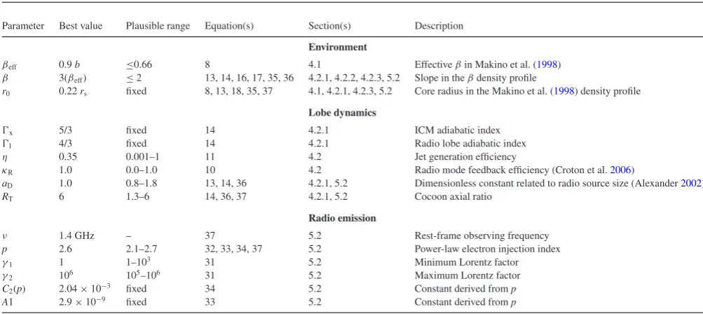
Table 1. The new AGN model parameters, their best values, plausible ranges, equation number(s), section(s) and a brief description, as used throughout this paper.

Parameter Best value Plausible range Equation(s) Section(s) Description Environment

βeff 0.9b ≤0.66 8 4.1 Effectiveβin Makino et al. (1998)

β 3(βeff) ≤2 13, 14, 16, 17, 35, 36 4.2.1, 4.2.2, 4.2.3, 5.2 Slope in theβdensity profile

r0 0.22rs fixed 8, 13, 18, 35, 37 4.1, 4.2.1, 4.2.3, 5.2 Core radius in the Makino et al. (1998) density profile

Lobe dynamics

x 5/3 fixed 14 4.2.1 ICM adiabatic index

l 4/3 fixed 14 4.2.1 Radio lobe adiabatic index

η 0.35 0.001–1 11 4.2 Jet generation efficiency

κR 1.0 0.0–1.0 10 4.2 Radio mode feedback efficiency (Croton et al.2006)

aD 1.0 0.8–1.8 13, 14, 36 4.2.1, 5.2 Dimensionless constant related to radio source size (Alexander2002)

RT 6 1.3–6 14, 36, 37 4.2.1, 5.2 Cocoon axial ratio

Radio emission

ν 1.4 GHz – 37 5.2 Rest-frame observing frequency

p 2.6 2.1–2.7 32, 33, 34, 37 5.2 Power-law electron injection index

γ1 1 1–103 31 5.2 Minimum Lorentz factor

γ2 106 105–106 31 5.2 Maximum Lorentz factor

C2(p) 2.04×10−3 fixed 34 5.2 Constant derived fromp

A1 2.9×10−9 _{fixed 33 5.2 Constant derived fromp}

AGN observations. Beyond a certain point, adding more parameters typically makes the model harder to calibrate.

4.1 The hot gas density profile and cooling

InSAGEevery dark matter halo is assumed to carry its cosmic share of

baryons, taken to befb=0.17, consistent with the WMAP1 results

of Spergel et al. (2003). These baryons begin their life as diffuse hot gas with primordial composition around the galaxy. However, as mentioned above, with time the gas transforms under the action of the many and varied physical processes of galaxy evolution to populate gas reservoirs of several different phases, as well as stars, black holes and the heavy elements (Baugh et al.2007).

Considering first this hot gas in virial equilibrium, its temperature can be described by (Sutherland & Dopita1993)

Tvir=

1 2

μmp

kB

V_circ2 , (1)

wherempis the mass of proton,μis the mean molecular weight of

gas,kBis the Boltzmann constant, andVcircis the circular velocity

at the virial radius of halo. In what follows we approximateVcircby

Vvirof the halo. Of course, after an AGN jet ploughs through this

gas it is unlikely to be in equilibrium, at least for a time. The new hot temperature of such gas is discussed in the following sections by taking into account the size and properties of an expanding shocked gas bubble due to an AGN outflow.

The hot gas density profile is similarly important as it directly determines the cooling (i.e. feeding) rate of gas into the galactic disc gas, which ultimately leads to the formation of new stars. The originalSAGEmodel, like many other semi-analytic models before it,

assumed that this hot gas can be represented as a simple isothermal sphere with temperature given above, and having a density profile (White & Frenk1991)

ρ(r)= mhot 4πRvirr2

. (2)

Heremhotis the total hot gas mass in the halo within the virial radius,

Rvir.

However this approximation is clearly an oversimplification, es-pecially when compared to X-ray observations of nearby cluster systems which show that the density profile is better described by an isothermalβmodel (Cavaliere & Fusco-Femiano1978; Fukazawa, Makishima & Ohashi2004; Pointecouteau et al.2004; Vikhlinin et al.2006),

ρ(r)= ρ0 [1+(r/rc)2]3β/2

, (3)

whererc defines a characteristic core radius andβdescribes the

changing inner and outer slopes of the profile.

For the purpose of this study, we adopt the density profile described by Makino, Sasaki & Suto (1998). The Makino pro-file closely matches the observationally fit β model given by equation (3), albeit based on a better theoretical foundation. It char-acterises the mass distribution that arises from isothermal gas in hy-drostatic equilibrium analytically embedded in a universal ‘NFW’ (Navarro, Frenk & White1996) dark matter halo. Again we assume that the gas is at the virial temperature of the halo. While a more re-alistic model would include a clustercentric radius-dependent tem-perature (e.g. Arnaud et al.2010), we adopt a single-temperature model to minimize the number of free parameters. Using this model, Makino et al. (1998) predict the core density, core radius,β param-eter and X-ray luminosity of clusters as function of halo mass and temperature. The Makino profile is given by

ρ(r)=ρ0e−27b/2(1+r/rs)27b/(2r/rs). (4)

Hereρ0is the core density of hot gas, whilersis the usual NFW

scale radius. If one assumes the hot gas is at the virial temperature of the halo (equation 1), thebparameter can be written as

b= 2C 9γ

ln (1+C)− C 1+C

−1

(5)

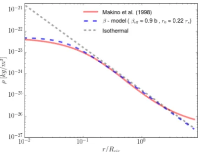
Figure 1. The hot gas density profile as a function ofr/Rvirfrom Makino

et al. (1998) (red solid line) and the original SAGE isothermal profile (grey short-dashed line). Densities are normalized to have the same total hot gas mass (mhot=1013h−1M). The best-fittingβprofile, withβeff=0.9band

r0=0.22rs, is also plotted with the blue long-dashed line for comparison.

C=Rvir/rs, was empirically determined by Bullock et al. (2001) to

be

C= 4 1+z

Mvir

1.4×1014_M

−0.13

(6)

withzthe halo’s redshift. Finally, the central density of the hot gas, ρ0, can be determined by integrating the Makino density profile out

to the halo virial radius and requiring the total mass equalmhot:

ρ0=

mhot

4πr3 s

e27b/2

C

0

x2(1+x)27b/2x_dx −1

, (7)

where we have used the change of variablex≡r/rs.

We can combine the above Makino profile representations forb (equation 5),rs=Rvir/C(using equation 6) andρ0(equation 7) to

obtain aβ-model-type expression,

ρ(r)= ρ0A(b) [1+(r/rc,eff)2]3βeff/2

. (8)

The parameters completing the profile are:A(b)= −0.178b+0.982, r0 ≡ rc, eff = 0.22rs and βeff = 0.9b, all valid over scales

0.01rs<r<10rs.

In Fig.1we compare the density profile of Makino et al. (1998) (equation 4, red solid line) to that of theβmodel (equation 3, blue long-dashed line) as function of radius (in units ofRvir) for the same

total hot gas mass (mhot=1013h−1M). Also overplotted is the

original isothermal profile (∝1/r2_{) used inSAGE(equation 2, grey}

short-dashed line). The Makino andβ-model profiles agree com-fortably well across the entire range plotted, while the isothermal profile is seen to deviate significantly from the other two on scales less than∼0.1Rvir, where cooling is most significant.

4.2 Jet generation and propagation

Following the original model described in Croton et al. (2006), the accretion rate of gas feeding the black hole is approximated by the Bondi–Hoyle formula (Bondi1952),

˙ mBH=

2.5πG2_m2 BHρ0

c3 s

, (9)

wheremBHis the black hole mass andρ0is the density of accreting

hot gas around the black hole.cs≡VvirandGare the speed of sound

in the gas and the gravitational constant, respectively.

The key unknown above is the central gas density, which can be approximated by assuming a maximal cooling flow in this region, as explained in section 9.1 of Croton & Stevens (2016). This leads to an expression forρ0that can be inserted back into equation (9),

after which the accretion rate simplifies to

˙ MBH=κR

15 16πGμmp

kT

λ MBH. (10) Equation (10) is now written in terms of quantities thatSAGE

nat-urally produces. Note that the efficiency parameter,κR, was

intro-duced by Croton & Stevens (2016) to modulate the effectiveness of the feedback within the cooling–heating cycle.

Moving beyond this original accretion implementation, we look to build a physical model of the outflows produced as a result of gas accretion on to a black hole. There are two different accretion states that can both happen when removing angular momentum from the accretion disc by viscosity (Narayan, Mahadevan & Quataert1998; Meier2001; K¨ording, Jester & Fender 2006; Fender, Belloni & Gallo2004). The ‘hot mode’ occurs for low accretion rates with respect to the Eddington rate ( ˙MBH< αcritM˙edd). Here, the flow

is geometrically thick and optically thin, which results in longer cooling times and more powerful jets (for a given black hole mass and accretion rate). The thermal energy of the inflowing gas is advected inward, known as an advection dominated accretion flow (ADAF; Narayan & Yi1995).

We relate ‘hot mode’ jet power to the accretion rate via the following relation:

Qjet,hot=ηM˙BHc2, (11)

wherecis the speed of light andηis the jet efficiency, estimated using relativistic magnetohydrodynamical simulations of jet gen-eration to have typical values between 0.002 and 1; the exact value is largely set by black hole spin (Benson & Babul2009). In Section 5.3, we use observations to constrain the best-fitting value ofηto 0.35.

In contrast, the ‘cold mode’ of AGN accretion occurs when inflow rates are high compared with the Eddington rate ( ˙MBH> αcritM˙edd).

Here, the accretion flow can be described by the standard thin disc solution of Shakura & Sunyaev (1973), where the disc is geomet-rically thin and optically thick. This produces outflows that are radiatively efficient and hence the AGN has weaker jets (for a given black hole mass and accretion rate) in comparison to the ADAF case (Narayan2002). The cold mode jet power is given by (Shakura & Sunyaev1973; Meier2001, Equation 5)

Qjet,cold=6.3×10−5

MBH

109_M

−0.1

˙

m0_BH.2( ˙MBHc2)[W], (12)

where ˙mBH≡ ˙

MBH ˙

Medd.

Note that the parameterαcrit defines the transition from hot to

cold accretion in units of the Eddington rate and is set at 0.03 throughout this work (see also Merloni & Heinz2008; Shabala & Alexander2009). In our model we generate both ADAF and thin disc jets with different jet generation efficiencies.

4.2.1 Radio source expansion

radio lobes to expand supersonically; this characterises the cocoon expansion, the evolution of which we now quantify.

Using the gas density profile described in Section 4.1, and as-suming a cocoon axial ratioRTfor a jet with kinetic powerQjet/2,

the dynamical model of Kaiser & Alexander (1997) characterises the evolution of the cocoon radius as

rcocoon(t)=aDr0

t τ

3/(5−β)

. (13)

Here time, t, is normalized to a characteristic time-scale, τ=

r₀5ρ0

Qjet

1/3

, while the dimensionless constant,aD, follows from the

work of Kaiser & Alexander (1997) and Shabala & Alexander (2009):

aD =

R4

T (x+1)(l−1)(5−β)3

18π9l+(l−1)R2T/2

−4−β 1/(5−β)

. (14)

Assuming a power-law density profile ofρ =ρ0(r/r0)−β for the

cocoon expansion where 0 < β < 2, and axial ratio between 1.3< RT < 6, the value foraD is in the range of 0.8–1.8 (see

Table1). We adoptaD=1, a value typical for radio sources in the

inner regions of clusters.

4.2.2 The cocoon shock radius

Following Kaiser & Alexander (1997), the relation between the maximum radius of the shocked gas and the radius of radio emitting cocoon plasma is given by

rshock=

1

λrcocoon, (15)

where the maximum radius is calculated using the AGN active time (ton, described below in Section 4.2.4) and the cocoon radius

(equation 13).λis dependent on the density profile, and we have assumed a self-similar solution for the shape of the cocoon,

1−λ3= 15

4(11−β). (16)

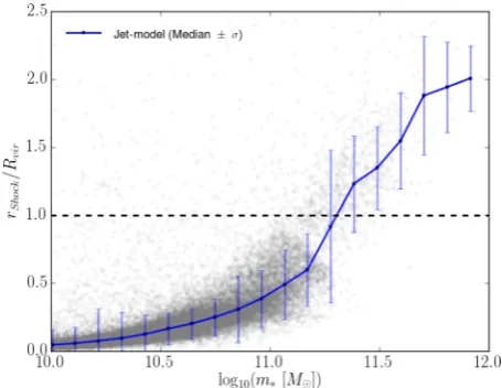
Observations show the existence of somewhat rare, extremely powerful AGN outbursts in massive galaxies (Rawlings & Jarvis 2004; Miley & De Breuck 2008; Shabala et al. 2011; Fabian2012). Their size extends many hundreds of kpc and their lifetimes can be up to 108_{yr (Shabala et al.2008). Radio sources}

sizes, denotedD, have a typical range of between 1 and∼1000 kpc (Willott et al.1999; Sadler et al.2007). In our model the shocked gas expands up to∼900 kpc, as can be seen in Fig.2, approximately consistent with such observations. Similarly, in Fig.3we show the distribution of shock radii as function of stellar mass. Together, these figures indicate that the AGN feedback can clear hot and cooling gas out to large radii. In our model, larger radio sources should preferentially be found in more dense environments. On the one hand, denser environments imply slower expansion speeds (through equation 13); on the other hand, more massive black holes found in such environments have both higher jet powers (equations 11, 12) and are longer lived (equation 24). As shown in Fig.2, the net effect is for larger radio sources to preferentially inhabit dense en-vironments in our model. Observationally, many large double-lobed radio galaxies are found in poor environments; on the other hand, many small-scale jets are also associated with Seyfert galaxies (e.g. Ulvestad & Wilson1984; Kaviraj et al.2015). The apparent com-pactness of many radio AGN may at least in part be due to the lack

Figure 2. Distribution of shocked radius as function of virial radius. The blue solid line presents the median of the individual model points, with standard deviation given by the error bar. The dashed black line indicates the limiting case when the shock radius extends out to the virial radius.

Figure 3. Shocked radius in units ofRviras function of stellar mass, as

shown by the grey data points for model central galaxies. The blue solid line presents the median of the individual model points, with standard deviation given by the error bar. The dashed black line indicates the limiting case when the shock radius extends out to the virial radius.

of sensitivity to diffuse low-surface brightness features in Fanaroff– Riley type I (FR I) radio galaxies (Shabala et al.2017). Our simple model cannot address this selection effect, which is deferred to future work. Given the simplicity of our model we resist the temp-tation to make more quantitative predictions than this, but it is an area for future work. The feedback is done in two ways, through heating of the gas and uplifting of the gas, which we describe in the following sections.

4.2.3 Gas heating and cooling

According to Alexander (2002), and following the study by Shabala & Alexander (2009), the difference between the mean isothermal temperature in the shocked gas and the post-shock temperature can be described by

Tshock=

15 16

3−β 11−β

μmH

kB

˙

Figure 4. New hot gas temperature in units ofTviras a function of stellar

mass. Results are show for central galaxies only, with the blue line and error bars indicating the median and standard deviation of the distribution in each stellar mass bin, respectively. The dashed black line indicates where the temperature remains at the virial value.

where the shock velocity is given by ˙rshock= ₅₋3_βrshock_ton , wheretonis

the active time of the AGN and is defined below in Section 4.2.4. We can then obtain the following integrated hot gas mass using the Makino et al. (1998) profile for a spherical shocked mass distribu-tion, given by

mshock(rshock)=16πρg0r03

ln

1+rshock r0

− rshock

rshock+r0

. (18)

The shocked mass can never exceed that of the mass of hot gas. When the gas is shock heated we assume an instantaneous mixing of this gas with the hot gas of the halo, resulting in a new hot halo temperature of

Tnew−hot=Thot+

mshock

mhot

(Tshock−Thot). (19)

Fig.4shows the distribution of this new hot gas temperature in units of the original virial temperature, given as a function of stellar mass. In general, AGN in our model act to raise the temperature of the gas by a few to 20 per cent, depending on the stellar mass of the central galaxy in the halo. In this model, we only change the temperature ifTshock>Tvir.

Hot halo gas is not static but cools over time. The cooling time of this gas at each radius is taken as the ratio of its specific thermal energy to the cooling rate per unit volume,

tcool(r)=

2 3

μmpkBTnew−hot

ρ(r)(Tnew−hot, Z)

, (20)

where(T,Z) is the cooling function and depends on the temper-ature,T, and metallicity,Z. In such models a cooling radiusrcool

is then defined as the radius at whichtcoolis equal to a

character-istic timescale of the system, such as its age, time since last major merger, or dynamical time. Following the standard implementation of SAGE we take the last of these.

For the so-calledhot accretion mode, whenrcool<Rvir, the

cool-ing rate of the hot gas is calculated uscool-ing

˙

mcool=4πρg(rcool)rcool2 r˙cool, (21)

Figure 5. A schematic of our intermittent physically motivated model for AGN feedback. The red line shows the time evolution of the jet. During the ‘on’ and ‘return’ phases only gas that has not been overrun by the shock can cool. During the ‘quiet’ phase cooling is allowed to proceed as usual (equation 29).

whereρg(rcool) is the Makino et al. (1998) profile gas density at the

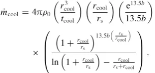
cooling radius. With this, the cooling rate can be rewritten as

˙

mcool=4πρ0

rcool3

tcool

rcool

rs

e13.5b 13.5b

×

⎛ ⎜ ⎜ ⎝

1+rcool

rs

13.5b

rs rcool

ln

1+rcool

rs

− rcool

rs+rcool

⎞ ⎟ ⎟

⎠. (22)

Alternatively, in the so-called cold accretion mode, when rcool >Rvir, the hot halo never forms and any infalling gas

cap-tured in the dark matter halo potential falls towards the centre on a free fall timescale,Rvir/Vvir, given by

˙ mcool=

mhot

Rvir/Vvir

. (23)

4.2.4 The AGN duty cycle and its effect on cooling

Left unchecked, massive dark matter haloes in particular can collect prodigious amounts of hot gas which will lead to runaway cooling at rates that are unsupported by the observations. Our AGN model provides an energy counterbalance to such cooling through the heating resulting from an AGN jet. Over long timescales (100s of Myr to many Gyr), such energy injection can be approximated as uniform and constant, as assumed in Croton et al. (2006). However, a more realistic model will attempt to describe the intermittent nature of black hole accretion and their resulting outflows and properties. To this end, suppose that we have a black hole of a given mass being fed gas from its surrounding medium through an accretion disc. We simplify the otherwise complicated resulting AGN duty cycle by breaking it into four primary parts: the time that the jet is on,ton, inflating the cocoon as described above; the switching off of

the AGN and hence jet when accretion stops; the time it takes for the cocoon to disappear once the jet pressure has been removed,treturn;

and finally the subsequent period of quiescence after the cocoon has dissipated but before the next episode of accretion reignites the AGN and jet,tquiet. This cycle is illustrated in Fig.5, and we

Observationally, the AGN fraction as a function of stellar mass was used by Turner & Shabala (2015) to estimate an expression for ton, approximately given by

ton=120

m∗

1011_M

0.7

Myr. (24)

Characteristic timescales forton range from between 2×107 to

5×108_{years for stellar masses between 10}10_{and 10}12_M

. For very-low mass galaxies this expression implies radio sources that are so small as to do no feedback.

Once support from the jet for the cocoon has been removed, the time for it to collapse back down can be estimated using the free fall time from the shock radius, which we parametrize as

treturn=2

rshock

cs

≈2rshock Vvir

. (25)

Here,csis the sound speed in the gas which we approximate

us-ing the virial velocity of the parent halo,Vvir. The factor of 2 is

an empirically chosen value we use to prevent overcooling in our model. Physically, the slow (slower than the sound speed) return of the shocked gas is due to processes we do not model here, such as the movement of buoyant bubbles once the jet switches off and the slow mixing of the heated gas throughout the cluster (Basson & Alexander2003; Soker2015; Yang & Reynolds2016).

The total time the AGN is off,toff, can be calculated from ton

using the observed duty cycle of AGN in the local Universe. Best et al. (2005) and Shabala et al. (2008) both measured the radio loud AGN fraction as a function of galaxy mass; using Fig.3of Best et al. (2005) the duty cycle can crudely be approximated as

δ=0.05

m∗

1011_M

1.5

, (26)

from whichtoffis simply

toff(m∗, ton)=ton

1 δ−1

. (27)

It then follows thattquietis just the difference between the total AGN

off time and the cocoon return time,

tquiet=toff−treturn. (28)

The presence of inflated cocoons from the AGN is expected to modify the cooling rate in the hot halo in multiple ways. For our model we make a simple approximation and suppress cooling whenever a cocoon is present, with the degree of suppression pro-portional to the hot gas mass fraction between the shock radius and cooling radius. In other words, only gas that has not been overrun by the shock can cool. This approximation is reasonable, as the active phase corresponds to at most a third of the total cycle time (see equation 26) and significantly less for lower mass galaxies. Further-more, jet driven bubbles uplift the shocked gas further away from the galaxy centre, thus stopping it from cooling. Once the cocoon expansion stops, gas can re-fill the evacuated cavity. If this ‘return’ time is less than the ‘off’ time, the system will experience a period of quiescence and cooling will be restored. Across the entire cycle the cooling rate may be further modified through the altered hot gas temperature (see Fig.4).

In summary, the time-averaged fraction of cooling in the presence of the AGN duty cycle is

fcool=

tquiet

ton+toff

+

ton+treturn

ton+toff

m(rcool)−m(rshock)

m(rcool)

. (29)

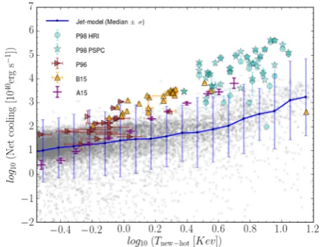
Figure 6. Net cooling rates as function of hot halo gas temperature atz=0. Grey data point show model central galaxies, with the blue line and error bars indicating their median plus standard deviation. Circled and starred points with error bars show the observational data of galaxy clusters from Peres et al. (1998, P98), measured with the High Resolution Imager and Position Sensitive Proportional Counter on ROSAT, respectively. Triangular points with errors show the observational data of galaxy groups from Ponman et al. (1996, P96) and Bharadwaj et al. (2015, B15). Stacked X-ray observations surrounding local brightest cluster galaxies from Anderson et al. (2015, A15) are shown with the horizontal lines with errors.

We include only the first term in the case of modified cooling due to jet heating that leads to higher hot gas temperatures, only the second term in the case of feedback and altered cooling from gas uplifting and both terms in the full model. The new cooling rate is given by

˙

mcool=fcoolm˙cool. (30)

5 R E S U LT S

5.1 Model constraints

Our AGN jet model makes three important changes to the previous SAGE radio-mode prescription. Namely, it uses a more realistic hot gas density profile to calculate cooling, the AGN jet can heat the hot gas to higher temperatures than before and the combined effect of this new temperature and the jet inflated cavities act to alter the cooling rate in a more realistic way. To calibrate this model we use a set of observables that the output must reasonably compare with, and that too in a physically sensible way. Only then can we extend our analysis to explore predictions and consequences that can be compared with future observations.

To start, in Fig.6we show the cooling rates from our model at z=0 as function of their hot halo gas temperature (equation 19). We compare with a number of X-ray observations of gas surrounding lo-cal galaxy clusters and groups: Ponman et al. (1996) and Bharadwaj et al. (2015), who evaluate the bolometric luminosity withinr500;

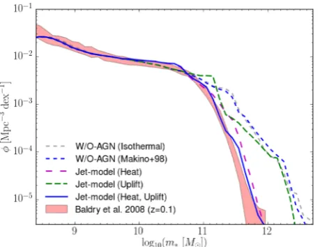
Figure 7. The stellar mass function of model galaxies for a range of different AGN assumptions. We highlight the local observed function from the SDSS using the red shaded region, as measured in Baldry, Glazebrook & Driver (2008). The original isothermal and Makino et al. (1998) density profiles with all AGN switched off are given by the grey dashed line and blue dashed line, respectively. The effect of using the new hot gas temperature (‘heat’) and AGN duty cycle (‘uplift’) are shown with the red and green long-dashed lines, respectively. The ‘heat’ and gas ‘uplift’ (see Section 4.2.4) prescriptions together are given by the blue solid line, our final model.

haloes, where we tend to under-predict cooling somewhat. The jet model fares considerably better than the original Croton et al. (2006) and Croton & Stevens (2016) models, which over- and under-predict these observations by a significant amount, respectively (Croton & Stevens2016, see e.g. their fig. 7).

The consequence of cooling is a pooling of cold gas in the galactic disc which then leads to star formation (see e.g. Croton et al.2006). A key motivator to include AGN feedback in semi-analytic models is to understand how the suppression of this infalling gas then leads to a suppression of the formation of new stars. The effectiveness of this feedback, and at the right mass scale, is usually quantified using the galaxy stellar mass function, the shape of which is moulded by both AGN and supernovae. As in previous works, we use the high mass end and knee of the local stellar mass function to constrain our jet model (the low mass end is constrained by other feedback processes and not the focus of the present work).

Fig.7shows the effect of the jet model on the formation of high mass galaxies compared to the Sloan Digital Sky Survey (SDSS) observations of Baldry et al. (2008). First we present the stellar mass function for the original SAGE model without any AGN feedback (grey dashed line) then systematically add the changes described in the previous sections until we arrive at our default version. This version includes the updated hot gas density profile (blue short-dashed line) and both gas heatings by the AGN jet (red long-short-dashed line) and also mass transport through uplifting (blue solid line, our final model).

Lastly, we consider the star formation rate density evolution of the galaxy population with time. In Fig.8we plot the final model by the blue line and two bounding cases: the original SAGE model (magenta long-dashed line) and our model but with AGN feedback turned off (grey short-dashed line). As can be seen, both SAGE and our new jet model matches the observational compilation of Somerville, Primack & Faber (2001) reasonably well. This is in contrast to when AGN feedback is turned off, which overproduces star formation at all redshifts except the highest.

Figure 8. The average star formation rate density history of the Universe produced using our jet model (blue line), compared to observational com-pilation from Somerville et al. (2001) (red points), the Croton & Stevens (2016) model (magenta long-dashed line) and our model with AGN feedback switched off (grey short-dashed line).

5.2 Deriving radio luminosities

We now consider the AGN properties of our model galaxies, a new feature of this work, with a focus on comparing with observables. In particular, we look at the cocoon shock size, jet power, and 1.4 GHz radio luminosity.

In our model the jet is assumed to expand into a hot atmosphere with a Makino density profile, characterized by core radiusr0, core

densityρ0and power-law outer slopeβeff (see Section 4.1). The

resulting radio lobes can be seen by their synchrotron emission. This depends on the cocoon magnetic field energy density,uB, the

distribution of Lorentz factorsγof the emitting electrons,n(γ) and cocoon volume,V. The energy due to the emission of synchrotron radiation is mostly injected at the hotspot between a minimum and maximum Lorentz factor,γ1 andγ2, with the initial energy

distribution given by

n(γi)=keγ−

p

i . (31)

The electrons inflate the radio-emitting cocoon and lose energy through adiabatic expansion, synchrotron emission and inverse Compton upscattering of cosmic microwave background photons.

Following Kaiser & Best (2007) and Shabala & Godfrey (2013) under the assumption of equipartition between particle and magnetic field energy density the cocoon radio luminosity at frequencyνcan be written

Lν =A1u 5+p

4

B V ν

1−p 2 ₍₁+_z)

(3−p)

2 _{, (32)}

wherepis the power-law index of the electron energy distribution andα=(1−p)/2. Using the definition of the spectral index for synchrotron emission,Fν∝να, a reasonable hotspot value for radio galaxies withαbetween−0.55 and−0.85 isp=2.1−2.7.

A1is a numerical constant given by

A1=

16π2_r e

c

q me

(p+1) 2

(2μ0) (p+1)

4 C2(p)

f(p, γ1, γ2)

, (33)

wherere is the classical electron radius, qand me are the

Figure 9. The distribution of radio luminosity as a function of shock radius weighted by AGN active time,ton, and colour coded by the abundance of

size-luminosity pairs in each bin size. The blue line and error bars indicate the median and standard deviation of the central galaxies in the model atz

=0, respectively.

space andf(p, γ1, γ2)=

γ2

γ1 γ

1−p_{dγ. The functionC}

2(p) can be

expressed as

C2(p)=

3p/2

2p+213π p+2

2

fn

p+1 4

fn

p

4+ 19 12

fn

p

4− 1 12

fn

p+7 4

. (34)

Here,fn(z)=

∞ 0 t

z−1_e−t_{dtis the Gamma function (Worrall2009)} and forp=2.6,C2(p)=2.04×10−3. The results explored in this

paper assume the best values described in Table1.

For self-similar expansion, the cocoon volume isV =πR2 TD

3_,

whereRTis the axial ratio of the source taking values between 1.3

and 6 (Leahy & Williams1984; Leahy, Muxlow & Stephens1989), andD=2rshockis the diameter of the cocoon. It can be shown that

the magnetic field energy density, which is proportional to the co-coon pressure, can be written (Kaiser & Alexander1997; Kaiser & Best2007,2008; Shabala & Godfrey2013) as

uB=

rfp (r+1)(l−1)

ρ0r

β

0

Qjet

2 21/3

(2rshock)−(4+β)/3, (35)

wherer= p+1₄ , and the constantfpis taken from Kaiser & Best

(2007),

fp=

18a2(5_D−β)/3 (x+1)(5−β)2RT2

. (36)

The radio luminosity is then

Lν =A1πRT2

rfp (r+1)(l−1)

(5+p) 4

ν(1−p)/2

×(1+z)3−2p

ρ0r0β

Qjet

2

25+12p

×(rshock) 3−4+β

3 _5+p

4

, (37)

Here,Qjetis the total kinetic power from both radio jets.

For a given ton, higher jet powers yield both larger sizes

(equations 13 and 15) and radio luminosity (equation 37). In Fig.9

we show the predicted luminosity-size relation, weighted by AGN

Figure 10. The model relationship between derived 1.4 GHz radio lumi-nosity and jet power,Qjet. Grey data points show the prediction for central

galaxies in the model, while the blue line and error bars show the median and standard deviation of the points, respectively. This is compared to the observed cavity relation derived by Cavagnolo et al. (2010) (black dashed line) and Heckman & Best (2014) (black solid line).

active time,ton. This figure illustrates that most sources have

pre-dicted sizes between 30–100 kpc and luminosities <1023_W/Hz.

In calculating the radio luminosities below, we adopt the final lu-minosity at ageton, rather than sampling different points along the

size-luminosity track. We adopt this simple treatment due to the lim-ited time resolution (260 Myr) of the SAGE output. In future work, we plan to include a more accurate sampling of the luminosity-size tracks. Furthermore, we have made the standard assumption that the synchrotron emitting electrons in the radio lobes are in the minimum energy state, i.e. there is approximate equipartition between the magnetic field and particle energy densities. Obser-vational evidence (e.g. Croston et al. 2005; Shelton, Hardcastle & Croston2011; Hardcastle & Krause2014) suggests that most sources have sub-equipartition magnetic fields, and the departure from the equipartition value depends on a number of factors includ-ing radio source morphology. Croston et al. (2005) quote median magnetic field values that are marginally sub-equipartition, 0.7Beq.

Adopting this in our work would decrease the radio luminosities by a factoru(5B+p)/4∼0.5, i.e. a factor of 2 lower.

5.3 Radio AGN properties

Fig.10shows the relation between jet power,Qjet, and 1.4 GHz radio

luminosity. Our results are consistent with that found by Cavagnolo et al. (2010) and Heckman & Best (2014) given by the solid and dashed black lines, respectively. We note that Heckman & Best (2014) estimate the jet mechanical energy of radio sources from the observed cavities and bubbles in the X-ray gas.

Figure 11. The model radio luminosity function in two redshift bins ofz= 0 andz=1. We compare to the observational results of Best & Heckman (2012) in the local volume (red shading) and 0.7–1.0 (blue shading).

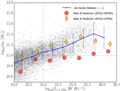
Figure 12. The model stellar mass-radio luminosity relation distribution compared with the observations of HERGs and LERGs from Best & Heckman (2012). Grey data points show the prediction for central galax-ies in the model (which we expect to be LERGs), while the blue line and error bars indicate the median and standard deviation of the points, respec-tively. Dashed lines show the approximate completeness limits of the Best & Heckman (2012) sample.

it produces roughly the right abundances atz=1 is encouraging. Of course, the model is built from parts which approximate highly complex physical phenomena, and in the future we plan to use better ones – for example a more holistic density profile for cooling and AGN expansion. Such sophisticated approaches to predicting the radio AGN properties (e.g. Turner & Shabala2015) are deferred to future work.

In Fig. 12 we investigate the observed radio luminosity as a function of stellar mass, again comparing our model against the data of Best & Heckman (2012). Here the grey symbols show the model AGN distribution, with the line and error giving the median and scatter. As can be seen, our model is more aligned with the observed properties of low excitation radio galaxies (LERGs) across most of the stellar mass range plotted, which are fuelled by cooling flows, although at the lowest masses our model galaxies could be made up of a mix with high excitation radio Galaxies (HERGs). The Best

& Heckman (2012) sample extends toz=0.3, which corresponds to a completeness of approximately 1024_{W/Hzat 1.4 GHz in radio}

luminosity (using the 99 per cent NRAO VLA Sky Survey (NVSS) completeness cutoff of 3.4 mJy), and 1011_M

in stellar mass (using a SDSSr-band magnitude limit of 17.77 and the relations of Bell et al.2003). These observations are therefore likely to be complete in stellar mass for the bulk of the bright LERG population, however not for HERGs where the observed median masses should be treated as upper limits.

6 D I S C U S S I O N A N D C O N C L U S I O N S

In this work we present a new prescription for AGN feedback that models in a more realistic way the intermittent nature of black hole accretion in the galaxy population and its resulting outflows. This update is built upon the SAGE semi-analytic galaxy formation model described in Croton & Stevens (2016), which itself was an update to the model that introduced the original ‘radio mode’ semi-analytic prescription in Croton et al. (2006). Our enhancements extend to gas cooling from the hot halo to make the cooling–heating cycle self-consistent, and include a new hot gas density profile that is better aligned with that observed in X-ray clusters. Overall, and after some minor parameter retuning, our additions retain the good fit SAGE has to a number of key galaxy population statistics, like the stellar mass function (for which AGN heating is critical at the high-mass end) and star formation rate density evolution, while expanding the number of observables it can make predictions for, in particular for AGN and radio galaxies.

Unlike most semi-analytic approaches, the AGN energy injec-tion in our model is spatially distributed. Omma & Binney (2004) pointed out that, for large radio sources, much of the AGN kinetic power can be wasted by coupling to hot gas at large cluster-centric radii, which has long cooling times. By modelling the dynamical evolution of jet-inflated structures explicitly, we address this issue. In this, new model AGN and its resulting feedback are followed through a number of key phases with time: (1) black hole accretion acts to turn on a jet, which quickly expands into the surrounding hot halo gas and inflates a cocoon; (2) after a period of time the accre-tion stops, and hence also the jet, which removes pressure support from the cocoon leading to its deflation (return), and ultimately dissipation; and finally (3) the galaxy then undergoes a period of quiescence, which lasts until accretion on to the black hole is re-established, after which the cycle begins again. Importantly, only during the quiet phase do we allow cooling of gas on to the galaxy, with the duration of this time set by our prescriptions for the AGN jet on, off and cocoon return times.

Within our model, gas heating from an AGN jet acts to raise the mean temperature of the hot halo by up to∼20 per cent above the virial temperature (Fig.4). When compared to the previous SAGE model, we obtain a superior match to the observed cooling luminosity X-ray hot gas temperature relation, although we tend to under-predict the observations for the most massive clusters (Fig.6). Our more realistic cooling rates follow from the combined effect of the modified hot gas temperature and the influence that the jet inflated cavities have on the movement of this gas.

with the LERG population, rather than the HERG population, when compared with the observations of Best & Heckman (2012). In-deed, we can match the stellar mass function in a number of ways, but to match the radio luminosity function as well we find our free parameters, as given in Table1, must be chosen to produce AGN with LERG-like properties.

However our model is not without its simplifications and areas for improvement. For example, the model only follows the active phase of jet inflated cavities and not the rising buoyant bubbles that can influence the hot gas long after the AGN has switched off (as seen from X-ray cavities with radio emission). Thus, our sources may better represent a population of FR IIs, and our model mayunderestimatethe total amount of feedback done by the AGN. In addition, we ignore the possibility of sound waves distributing heating to large radii. On the other hand, we have also assumed that all cavities have simple morphology with a covering factor of 1. In reality, cavities show complicated shapes, with material constantly falling back in behind. As such, these assumptions will tend tooverestimatethe efficiency of feedback. Alexander (2002) considered the evolution of the swept-up shell of shocked gas, and showed that the cooling time of the swept up gas depends sensi-tively on the thermal conductivity of the cluster. In the case that the shocked gas evolves isothermally (as would be the case for clusters in which thermal conductivity is not suppressed), radiative cooling was shown to only be significant in the centres of cool core clusters. On the other hand, the shocked gas can cool rapidly if it evolves adiabatically. Our results suggest that thermal conductivity in clus-ters may provide an important feedback mechanism, as previously suggested by other authors (e.g. Narayan2002; McCourt, Quataert & Parrish2013).

Finally, it is important to note that although there is a consistency between our model predictions and observations in theQjet−Lradio

relation (Fig.10), this relation derived from observations of X-ray cavities suffers strongly from selection effects (Godfrey & Shabala2016). A relation based on dynamical models of radio AGN (Turner & Shabala2015) is not subject to such selection effects, but most likely provides a lower limit on the jet power for a given radio luminosity because of the assumption of an equipartition mag-netic field in the radio cocoon. Inverse-Compton observations (e.g. Croston et al.2005; Shelton et al.2011; Hardcastle & Krause2014) suggest that this assumption may overestimate the magnetic field strength by as much as a factor of 4. According to equation (35), a lower magnetic field would give a higherQjetfor the same radio

luminosity.

Despite these shortcomings, this paper presents a new effort to in-corporate the effects of AGN jet and cavity production into a cosmo-logical model of galaxy formation. Before we can make predictions for future radio surveys we first need to have a well-constructed cosmological radio AGN model that produces a population which matches a baseline set of key statistics. The majority of our figures are calibration plots, demonstrating that our model construction and parameter choices by-and-large achieve this (for the properties considered at least).

This model is able to produce catalogues of both normal and ra-dio galaxies across a wide range of mass scales and environments, describing their evolution from high redshift down to the present day. Such catalogues offer a valuable resource for survey teams as they analyse current data and plan for the future. Extensions to our current work will focus on the geometry of bubble evolution (e.g. how do bubbles ‘pancake’ and sweep out the gas), how gas refills behind the bubble as it evolves and how the local magnetic field helps stabilize the bubble and delays gas from returning. To achieve

such detail we will employ more sophisticated high resolution nu-merical simulations, with the results then generalized and folded into our semi-analytic model, expanding its predictive power and usefulness to the community.

AC K N OW L E D G E M E N T S

We thank the anonymous referee for their constructive comments and suggestions which helped to improve the paper. MR is grateful to Swinburne University and its Centre for Astrophysics and Su-percomputing for hosting his stay during which much of this work was carried out. SS thanks the Australian Research Council for an Early Career Fellowship (DE130101399).

The Semi-Analytic Galaxy Evolution (SAGE) model that served as a basis for this work is a publicly available codebase that runs on the dark matter halo trees of a cosmological N-body simulation. It is available for download at https://github.com/

darrencroton/sage. The Millennium Simulation on which the

semi-analytic model was run was carried out by the Virgo Supercomput-ing Consortium at the ComputSupercomput-ing Centre of the Max Plank Soci-ety in Garching. It is publicly available online at

http://www.mpa-garching.mpg.de/Millennium/ through the German Astrophysical

Virtual Observatory.

R E F E R E N C E S

Alexander P., 2002, MNRAS, 335, 610

Anderson M. E., Gaspari M., White S. D. M., Wang W., Dai X., 2015, MNRAS, 449, 3806 (A15)

Arnaud M., Pratt G. W., Piffaretti R., B¨ohringer H., Croston J. H., Pointe-couteau E., 2010, A&A, 517, A92

Bahcall J. N., Kirhakos S., Saxe D. H., Schneider D. P., 1997, ApJ, 479, 642 Baldry I. K., Glazebrook K., Driver S. P., 2008, MNRAS, 388, 945 Banfield J. K. et al., 2016, MNRAS, 460, 2376

Barthel P. D., Arnaud K. A., 1996, MNRAS, 283, L45 Basson J., Alexander P., 2003, MNRAS, 339, 353

Baugh C. M., Lacey C. G., Frenk C. S., Granato G. L., Silva L., Bres-san A., Benson A. J., Cole S., 2007, in Baker A. J., Glenn J., Harris A. I., Mangum J. G., Yun M. S., eds, ASP Conf. Ser. Vol. 375, From Z–Machines to ALMA: (Sub)Millimeter Spectroscopy of Galaxies. As-tron. Soc. Pac., Charlottesville, Virginia, p. 7

Begelman M. C., Cioffi D. F., 1989, ApJ, 345, L21

Bell E. F., McIntosh D. H., Katz N., Weinberg M. D., 2003, ApJS, 149, 289 Bender R., Saglia R. P., 1999, in Merritt D. R., Valluri M., Sellwood J. A., eds, ASP Conf. Ser. Vol. 182, Galaxy Dyanmics. Astron. Soc. Pac., San Francisco, p. 113

Benson A. J., Babul A., 2009, MNRAS, 397, 1302 Best P. N., Heckman T. M., 2012, MNRAS, 421, 1569

Best P. N., Kauffmann G., Heckman T. M., Ivezi´c ˇZ., 2005, MNRAS, 362, 25

Best P. N., Ker L. M., Simpson C., Rigby E. E., Sabater J., 2014, MNRAS, 445, 955

Bharadwaj V., Reiprich T. H., Lovisari L., Eckmiller H. J., 2015, A&A, 573, A75 (B15)

Bˆırzan L., Rafferty D. A., McNamara B. R., Wise M. W., Nulsen P. E. J., 2004, ApJ, 607, 800

Bˆırzan L., McNamara B. R., Nulsen P. E. J., Carilli C. L., Wise M. W., 2008, ApJ, 686, 859

Blandford R. D., Payne D. G., 1982, MNRAS, 199, 883 Blandford R. D., Znajek R. L., 1977, MNRAS, 179, 433

B¨ohringer H., Voges W., Ebeling H., Schwarz R. A., Edge A. C., Briel U. G., Henry J. P., 1991, NATO Advanced Science Institutes (ASI) Series C, 348, 293