Advance Access publication 2018 November 30
On the dynamics of the Small Magellanic Cloud through high-resolution
ASKAP H
I
observations
E. M. Di Teodoro ,
1‹N. M. McClure-Griffiths,
1K. E. Jameson,
1H. D´enes ,
1,2,3John M. Dickey,
4S. Stanimirovi´c,
5L. Staveley-Smith ,
6,7C. Anderson ,
2J. D. Bunton,
2A. Chippendale ,
2K. Lee-Waddell ,
2A. MacLeod
2and
M. A. Voronkov
21Research School of Astronomy and Astrophysics – The Australian National University, Canberra, ACT 2611, Australia 2CSIRO Astronomy and Space Science, PO Box 76, Epping, NSW 1710, Australia
3ASTRON – Netherlands Institute for Radio Astronomy, NL-7991 PD, Dwingeloo, The Netherlands 4School of Natural Sciences, University of Tasmania, Hobart TAS 7001, Australia
5Department of Astronomy, University of Wisconsin, Madison, WI 53706, USA
6International Centre for Radio Astronomy Research (ICRAR), University of Western Australia, Crawley, WA 6009, Australia 7ARC Centre of Excellence for All Sky Astrophysics in 3 Dimensions (ASTRO 3D), Australia
Accepted 2018 November 12. Received 2018 November 5; in original form 2018 September 26
A B S T R A C T
We use new high-resolution HIdata from the Australian Square Kilometre Array Pathfinder to investigate the dynamics of the Small Magellanic Cloud (SMC). We model the HIgas component as a rotating disc of non-negligible angular size, moving into the plane of the sky, and undergoing nutation/precession motions. We derive a high-resolution (∼10 pc) rotation curve of the SMC out toR ∼4 kpc. After correcting for asymmetric drift, the circular velocity slowly rises to a maximum value of Vc55 km s−1 at R2.8 kpc and possibly flattens outwards. In spite of the SMC undergoing strong gravitational interactions with its neighbours, its HIrotation curve is akin to that of many isolated gas-rich dwarf galaxies. We decompose the rotation curve and explore different dynamical models to deal with the unknown 3D shape of the mass components (gas, stars, and dark matter). We find that, for reasonable mass-to-light ratios, a dominant dark matter halo with massMDM(R <4 kpc)1–1.5×10⁹M is always required to successfully reproduce the observed rotation curve, implying a large baryon fraction of 30 per cent–40 per cent. We discuss the impact of our assumptions and the limitations of deriving the SMC kinematics and dynamics from HIobservations.
Key words: galaxies: dwarf – galaxies: kinematics and dynamics – Magellanic Clouds.
1 I N T R O D U C T I O N
The Large and Small Magellanic Clouds (LMC and SMC) are gas-rich dwarf satellites of the Milky Way (MW). The interactions of the Magellanic Clouds (MCs) with each other and with the MW (Besla et al.2010, 2012) have produced the Magellanic Stream (Mathewson, Cleary & Murray1974), a trail of gas extending more than 180◦across the sky, including the Leading Arm. The ongoing LMC–SMC interaction is furthermore clearly shown by the stream of gas and stars linking the two galaxies, commonly referred to as Magellanic Bridge (e.g. McGee & Newton1981). These gravita-tional interactions have had a significant impact on the history of the MCs (e.g. Putman et al.1998) and both their present-day
E-mail:[email protected]
phology and dynamics are highly complex and heavily disturbed. Studying the current properties of the MCs is the key to understand their recent evolution and interaction mechanisms with the MW.
As the least massive component of the interacting system, the SMC is the most easily affected by tidal forces and therefore shows the most peculiar features. Stars and gas in the SMC appear to behave very differently from a structural and kinematical point of view. On the plane of the sky, most of the stars lie along a bar-like structure, extending from the north-east to the south-west direction, but the real 3D shape of the SMC is still very uncertain. Old and intermediate-age stellar populations are thought to be distributed in a spheroid or ellipsoid significantly elongated along the line of sight (LOS) with the north-eastern region of the bar being closer to us than the south-western region (e.g. Hatzidimitriou & Hawkins1989; Cioni et al.2000; Glatt et al.2008; Subramanian & Subramaniam
2012). Younger stellar populations seem instead to be configured in
a flatter disc-like structure possibly following the LOS orientation of the older stars (e.g. Subramanian & Subramaniam2015; Jacyszyn-Dobrzeniecka et al.2016; Ripepi et al.2017). It is however still debated whether the stellar components, in particular the young population, have some significant rotational motion or whether the system is primarily supported by velocity dispersion (e.g. Harris & Zaritsky2006; Evans & Howarth2008; Dobbie et al.2014; van der Marel & Sahlmann2016; Gaia Collaboration et al.2018).
Unlike the stars, the gas in the SMC appears to have features in common with a uniformly rotating disc. Even the very first single-dish radio observations of atomic hydrogen (HI) in the SMC (Kerr, Hindman & Robinson1954; Hindman, Kerr & McGee1963) re-vealed that the gas has a significant velocity gradient along the stellar bar, pointing to possible circular motions, and attempts to derive the rotation curve of the SMC were soon made (Hindman
1967). More recently, interferometric data were obtained with the Australia Telescope Compact Array (ATCA, Staveley-Smith et al.
1997). This higher resolution data set (∼100 arcsec) revealed the complexity of the distribution and kinematics of the HIgas in the SMC, showing several hundred expanding shells, arcs and filaments underlying the large-scale rotation field (Stanimirovi´c et al.1999). Despite that, the ATCA data provided the best rotation curve for the SMC to date: Stanimirovi´c, Staveley-Smith & Jones (2004) showed that the SMC rotation curve linearly rises to a maximum circular velocityVc60 km s−1at a radiusR3 kpc and proposed a dy-namical model of the galaxy where stars and gas alone account for the observed rotation without the necessity of dark matter (DM). In a following paper, Bekki & Stanimirovi´c (2009) revised this dy-namical model and concluded that a dominant DM halo is instead needed to explain the rotation curve from Stanimirovi´c et al. (2004) work.
In this contribution, we update the SMC gas kinematics and dynamics using new high-resolution HIobservations carried out with the Australian Square Kilometre Array Pathfinder (ASKAP, DeBoer et al.2009). Using a generic model of a disc of arbitrary angular size and correcting for proper motion and asymmetric drift, we derive the rotation curve of the SMC with the highest linear resolution ever achieved for any extragalactic system (∼10 pc). We fit dynamical mass models to the observed rotation curve, testing the impact of assuming different density distributions for star, gas, and DM components, and we estimate the mass contribution of the DM halo within 4 kpc from the SMC centre.
The remainder of this paper is structured as follows. Section 2 describes the new ASKAP data and how we derive the kinematic maps that are used in the dynamical analysis of the SMC. Section 3 introduces the mathematical formalism and the set of equations needed to describe the velocity field of a rotating disc of non-negligible angular size onto the sky. We derive the rotation curve of the SMC in Section 4 and we decompose it into the contribution of the different mass components in Section 5. We compare our findings with previous studies of the gas kinematics in the SMC in Section 6. Approximations and caveats for our analysis and results are discussed in Section 7. We finally summarize and conclude in Section 8.
2 DATA
2.1 Observations and data reduction
The SMC was observed in the HI21-cm emission line with ASKAP as part of the Commissioning and Early Science observations. Data were obtained with 16 12-m antennas with baselines between 22 m
and 2.3 km during three consecutive nights (2017 November 3–5) for a total of approximately 36 h of integration time. Each antenna has 36 electronically formed beams arranged on a hexagonal grid on the sky, optimized for uniform sensitivity in a configuration calledClosepack36, which gives a field of view of about 20 deg2. Beams were formed with maximum signal-to-noise ratio weights determined via the method described in McConnell et al. (2016). The total bandwidth of the observations is 240 MHz divided into 12 960 channels of 18.5 kHz. Because we are only interested in a narrow band around the HIline, we immediately extract a sub-band from 1410 to 1430 MHz, which we used for the subsequent processing.
The data are calibrated using the ASKAPsoft Pipeline v0.19.51 (Whiting et al., in preparation), applied to each day of observation individually. The ASKAPsoft pipeline has two main calibration steps: (i) bandpass and absolute flux calibration and (ii) complex gain calibration, which relies on self-calibration techniques. Obser-vations with each beam of the primary calibrator PKS B1934−638 are used for bandpass and the primary flux scale. The per-beam bandpass solution measured on PKS B1934−638 is applied to the raw data. To accurately calibrate the complex gains, we mask out the channels containing bright HIemission from the SMC and the MW and form a continuum image of each beam from the remaining channels. For this masking we simply use the default 4σrms flag-ging threshold, beingσrmsthe root mean square (rms). We iteratively use the continuum images to solve for self-calibration solutions to the complex antenna-based gains. The self-calibration module of ASKAPSoft has three main steps: (i) the SELAVYsource-finding algorithm is run with an 8σrmsthreshold on the continuum image; (ii) the identified source components are used as input for the cali-bration to create a new gain solution; and (iii) the latest gain table is applied to the data and a new continuum image is produced . We repeat this self-calibration loop twice before creating the final continuum image and the final gain solutions, which are eventually applied to the unmasked, bandpass, and amplitude calibrated HI
visibility data. The self-calibration is only applied to the phases, while amplitudes are calibrated exclusively on PKS B1934−638. The calibrated data are used to image the HIemission line within theMIRIADdata reduction package (Sault, Teuben & Wright1995). We treat independent beams as individual pointings and image them with traditional linear mosaicking techniques and jointly decon-volve. During imaging, we use a Briggs’ visibility robustness pa-rameter of 0.8, which guarantees a good balance between natural and uniform weighting (Briggs 1995). The image is cleaned us-ing the maximum entropy deconvolution algorithm implemented in MOSMEM (Sault, Staveley-Smith & Brouw 1996), which is particularly appropriate for extended emission, unlike traditional Steer–Dewdney–Ito (Steer, Dewdney & Ito1984) clean. We allow
MOSMEMto run for 100 iterations or until the residuals reached the expected noise level of 1 mJy per beam. For most channels, the clean converges and no clean boxes are used. The restored ASKAP data cube was converted to a local standard of rest (LSR) spectral frame of reference and combined in Fourier space with the single-dish Parkes data from the HI4PI survey (HI4PI Collaboration et al.
2016). We note that the HI4PI single-dish data set is superior both
1The official release of ASKAPsoft can be foundhttps://doi.org/10.422
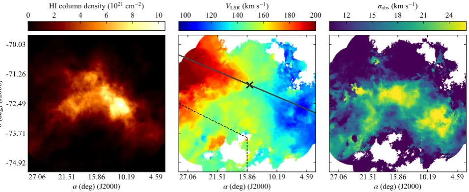
Figure 1. Maps extracted from the HIASKAP data cube of the SMC. From the left to the right, the column density map, the velocity field, and the observed velocity dispersion field. Maps have been derived as described in Section 2. On the velocity field, we show the best-fitting kinematic centre (black cross) and position angle of the LON (dark grey line) derived with the MCMC sampling (Section 4.1). The dashed line delimits the region toward the Magellanic Bridge masked out during the entire fitting procedure.
in coverage and sensitivity to the older Parkes data used in previous kinematic studies of the SMC (e.g. Stanimirovi´c et al.1999,2004). The final SMC data cube (ASKAP+Parkes) has a pixel size of 7 arcsec and a spectral channel width of 3.9 km s−1, with a restored beam size of 35 arcsec×27 arcsec full width at half-maximum (FWHM). The rms noise in brightness temperature per spectral channel isσrms=0.7 K.
2.2 Kinematic maps
We use the ASKAP+Parkes data cube to derive the HIcolumn density map, the velocity, and the velocity dispersion fields of the SMC to be used in the kinematic analysis. Regions of genuine emission are identified through the following procedure. We first convolve the data cube with a circular Gaussian kernel with FWHM of 70 arcsec, i.e. twice the beam major axis. A mask is then obtained using a flood fill algorithm, which starts from pixels with flux higher than 10σS, whereσSis the rms of the smoothed data cube, and floods regions down to 4σS. We visually check the mask and apply it to the original data cube to extract the moment maps. The zeroth moment M0is used to obtain the HIcolumn density map, i.e.NHI[cm−2]= 1.82×10¹⁸M0[K km s−1] (Roberts1975), under the assumption that the gas is optically thin. The first moment (i.e. the intensity-weighted mean velocity along the LOS) and the second moment are taken as velocity field and observed velocity dispersion field, respectively.
The derived maps are displayed in Fig. 1. The velocity field (central panel) shows a clear velocity gradient, with the LSR ve-locities going from about 90 km s−1in the south-west region to about 210 km s−1in the north-east region. This strong gradient and the quite regular iso-velocity contours perpendicularly to the major axis suggest that the large-scale motions of the gas are dominated by rotation. However, the velocity field looks disturbed, especially in the south-east region connecting to the Magellanic Bridge and along the galaxy minor axis, suggestive of non-circular motions possibly related to tidal interactions with the LMC and/or to gas outflowing from the SMC (McClure-Griffiths et al.2018). To avoid the areas with disturbed kinematics that might hamper our attempts
of deriving the underlying regular rotation, in our following kine-matic analysis, we mask out the south-east region enclosed by the black dashed line in Fig.1(the SMC ‘wing’) and we apply appropri-ate weighting functions to downweight regions close to the minor axis (see Section 4.2). The observed velocity dispersion (right-hand panel) varies between 10 and 25 km s−1, with the highest values towards the Magellanic Bridge and in correspondence of regions of star formation and supershells (Stanimirovi´c et al.1999). These val-ues include (i) the broadening due to thermal and turbulent motions, i.e. theintrinsicvelocity dispersion of the gas, (ii) the broadening due to geometrical effects when projecting onto the plane of the sky (e.g. in the case of a thick gas layer), and (iii) the instrumental broadening due to the finite spatial and spectral resolutions of a telescope. We finally stress that the maps shown in Fig.1do not include any correction for geometrical projection effects or proper motions of the SMC: those are directly taken into account during the modelling as described in the next section.
3 T H E O R E T I C A L F R A M E W O R K
Most kinematic studies of external galaxies assume that the ob-served object is at large distance, such that its angular size is small and a flat geometry over the area of the galaxy can be assumed (e.g. Begeman1989; Swaters1999; de Blok et al.2008). Although this is an appropriate assumption for most galaxies, the usual equa-tions used to model the velocity field in distant systems can be unsuitable to properly describe the observed kinematics of both the LMC and the SMC, which respectively subtend about 20◦and 6◦ on the sky. The geometric formalism to describe the velocity field of a rotating disc of arbitrary angular size was first introduced in the seminal papers by van der Marel & Cioni (2001) and van der Marel et al. (2002). Here, we summarize their main equations and we refer to these previous works for a comprehensive description of the geometry and the derivation of equations.
der Marel et al.2002, equation 24):
Vlos(ρ, )=Vsyscosρ+Vtsinρcos(−t)
+D0(∂i/∂t) sinρsin(−)
+f Vrot(R) sinicos(−) (1)
where the ingredients of the equation are as follows:
(i)ρ andare angular coordinates that identify the position on the celestial sphere of a point in a frame of reference centred on the CM:ρ is the angular distance from the CM andis the position angle with respect to the CM, measured anticlockwise from the north direction. Spherical trigonometry allows us to derive the angular coordinates from the equatorial coordinates (right ascension αand declinationδ) of any point for a fixed position of the CM (van der Marel & Cioni2001, equations 1– 3):
cosρ =cosδcosδ0cos(α−α0)+sinδsinδ0
sin=cosδsin(α−α0)/sinρ (2)
where (α,δ) and (α0,δ0) are the coordinates of the point and the CM, respectively.
(ii) Vsys,Vt, andtdescribe the motion of the CM in a frame of reference where the Sun is at rest:Vsysis the component along the LOS (positive when receding), often referred to assystemic velocity, Vtis the component perpendicular to the LOS, usually called trans-verse velocity, andtis the angle indicating the direction of the transverse motion on the celestial sphere, measured anticlockwise from north. For the SMC, the transverse velocity causes correc-tions ranging between±25 km s−1 across the velocity field (see Section 4.1).
(iii)D0is the distance of the CM from the Sun.
(iv)i and describe how the disc plane is viewed from our observing position:iis the inclination angle of the galaxy rotation axis with respect to the LOS (i= 0 for face-on view) andis the position angle of the line of nodes (LON), which identifies the intersection of the plane of the galaxy disc with the plane of the sky. In this work, we measureas the angle between the north direction and the receding part of the LON, taken counterclockwise.
(v)∂i/∂tis the time derivative of the inclination angle describing precession and nutation motions. We note that, unlike the inclination angle, variations of the position anglewith time do not affect the observed LOS velocity.
(vi) fis a geometrical factor, defined as:
f = cosicosρ−sinisinρsin(−)
(cos2icos2(−)+sin2(−))1/2 . (3)
(vii)Vrot(R) is the rotational velocity in the disc plane at cylin-drical radiusR=D0sinρ/f.
In practice, equation (1) tells us the expected value of the velocity field at each position (ρ,) for a rotating and precessing disc that is moving across the sky. In particular, the first two terms represent the LOS component of the CM velocity vector, the third term is the LOS component due to precession and nutation of the disc, and the last term is the LOS component of the rotation.
Equation (1) can be rewritten to take advantage of the knowledge on the measured galaxy proper motions towards the northμN≡ dδ/dtand towards the westμW≡ −(dα/dt)cosδdirections. Rear-ranging equation (1) leads to (equation 31 in van der Marel et al.
2002):
Vlos(ρ, )=Vsyscosρ+Wtssinρsin(−)
+(Vtcsinρ+f Vrot(R) sini) cos(−) (4) where:
Wts=Vts+D0(∂i/∂t) (5a)
Vts=Vtsin(t−)=D0μs (5b)
Vtc=Vtcos(t−)=D0μc (5c)
μs= −μWcos−μNsin (5d)
μc= −μWsin+μNcos . (5e)
In the above equations,VtcandVtsrepresent the projections of the tangential velocity along and perpendicularly the LON, respec-tively. Similarly,μcandμsare the projections of the CM proper-motion vector (μW,μN) along and perpendicular to the LON.
4 T H E HI K I N E M AT I C S O F T H E S M C
Equations (1) and (4) are functions of 10 unknown parameters: the centre coordinates (α0,δ0), the distanceD0, the inclinationiand LON position angle, the systemic velocityVsys, the transverse velocityVtand its directiont, the rotation velocityVrot and the precession/nutation term∂i/∂t. All these quantities but the rotation velocity refer to the disc in its entirety and can in principle be determined by fitting equations (1) or (4) to the observed velocity field. Conversely, the rotation velocity depends on the radiusR.
We therefore divided the problem of fitting the kinematics of the SMC in two steps. We first derive the global geometrical and kinematic properties of the SMC disc by comparing the observed velocity field to the modelledVlosvia a Monte Carlo Markov Chain (MCMC) sampling (Section 4.1). We then perform a tilted-ring analysis, where we decompose the velocity field in concentric rings at different radii and derive the rotation velocity as a function of R (Section 4.2). We finally correct the HIrotation curve for the asymmetric drift and obtain the circular velocity of the SMC (Section 4.3).
4.1 Global parameters of the SMC disc
Olszewski2008; Vieira et al.2010; Costa et al.2011), we decided to use the valuesμW = −0.772 ± 0.063 mas yr−1 and μN = −1.117±0.061 mas yr−1of Kallivayalil et al. (2013), based on three epochs ofHubble Space Telescopedata spanning 7 yr. Proper motions are used to calculate the transverse motion parametersVt, t,Vtc, andVtsthrough equations (5), reducing therefore the degen-eracy betweenVrot,Vtc, andi. We stress that the values of distance and proper motions assumed are much more accurate than what we may achieve with only the HIdata.
This first fitting step is meant to derive the global kinematic properties of the SMC disc and does not require a precise knowledge of the variation of the rotation velocity with radius. We make use of a simple, empirically motivated, and commonly used parametrization of the rotation curve:
Vrot(R)= 2
πVf arctan
R Rf
(6)
which rises nearly linearly until some scale radius Rf and then turns over and flattens to an asymptotic velocityVf. The function in equation (6) can describe the overall rotation pattern of a dwarf galaxy like the SMC with just two parameters,VfandRf.
The comparison between simulated and observed velocity fields is performed via an MCMC sampling, using the PYTHON im-plementation EMCEE by Foreman-Mackey et al. (2013). Differ-ently from a least-squares fitting, an MCMC estimates the pos-terior probability function for unknown parameters and gives a better handling of the correlations and uncertainties. We recall that the Bayes’ theorem states that, given a set of parameters x, the probability P(Vmod(x)|Vobs) of a model Vmod(x) given the observable Vobs is proportional to the product of the likelihood P(Vobs|Vmod(x)) and thepriorP(Vmod(x)) . An MCMC samples the parameter spacexin a way proportional to theP(Vmod(x)|Vobs), given the likelihood and the prior functions. In our case, x=
(α0, δ0, Vsys, i, , ∂i/∂t, Vf, Rf),Vmod(x)≡Vlos(x, ρ, ) given by equation (4) andVobsis the observed velocity field (Fig.1). We as-sume constant uninformative priors for all parameters and we define the likelihood function as:
logP(Vobs|Vmod(x))= − N
j=1 M
k=1
(Vlos(x, ρi, j)−Vobs(ρi, j))2 N×M
(7)
where the sums run over all theρandin the data [see equation (2)] andN×Mis the total number of non-blank pixels. We sample the posterior probability distribution with 500 walkers running 10 000 steps for each parameter, including a warm-up phase of 1000 steps. We check chains convergence using the integrated autocorrelation time as a diagnostic tool (e.g. Goodman & Weare2010).
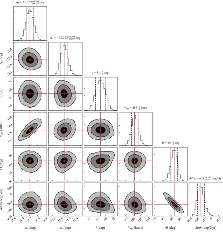
Fig. 2shows 2D marginalized posterior distributions (density plots) and the 1D joint posterior distributions (histograms on the di-agonal) for the MCMC sampling. Contours on the 2D distributions show the 1σ, 2σ, and 3σ confidence levels. We take the 50thper-centile value of the 1D posterior distributions as representative of the central value for each parameter (red solid lines), while lower and upper errors are taken at the 15.87th and 84.13thpercentiles (dashed lines), respectively. These values correspond to the mean and the standard deviation for a Gaussian distribution. Posterior distributions approach a Gaussian function for all parameters, in-dicating a well-attained sampling. The evident correlation between and∂i/∂tis due to the fact that the precession/nutation motions change the position angle of the LON.
The central value and error of each parameter are reported in Table1. Typical 1σuncertainties range between a few per cent (e.g. centre,Vsys) to about 40 per cent (∂i/∂t) of the central values. Some parameters estimated with our MCMC sampling appear to slightly differ from those previously derived by Stanimirovi´c et al. (2004) using HIATCA observations, although they are consistent within the errors. In particular, our kinematic centre is offset by 13 arcmin from theirs, we find a lower systemic velocity (157 versus 160 km s−1) and larger inclination (51◦versus 40◦) and position angle
(66◦versus 40◦). The position angle of 40◦used in Stanimirovi´c et al. (2004) is aligned with the stellar bar, but the HIgas major axis looks offset by more than 20◦from that value. The MCMC sampling returns a precession term of|∂i/∂t|=281 deg Gyr−1. This value represents the first attempt to derive the rate of change of the disc inclination angle from HIdata and it is a factor two larger than the value of 140 deg Gyr−1found by Dobbie et al. (2014) from the kinematics of red giant stars. However, given the large uncertainties associated with this parameter (see Table1and next paragraph), it is not possible to assert whether stars and gas are truly undergoing different precession motions or not.
Values given in Table1have been obtained by using proper mo-tions of Kallivayalil et al. (2013). In order to check the dependence of our best kinematic parameters on the assumed proper motions, we repeated the MCMC sampling using the measurements by Pi-atek et al. (2008), i.e. μW= −0.754 and−1.252 mas yr−1. We found that the central values of all parameters except∂i/∂tare in agreement to within<10 per cent. With proper motions from Piatek et al., we obtain a∂i/∂t= −171±120 deg Gyr−1, barely consistent with the one obtained with the values from Kallivayalil et al.. This is a further confirmation that the magnitude of precession/nutation motions is not well constrained with the present analysis and should be read as a rough estimate rather than a precise measurement. We finally stress that the value of∂i/∂tdoes not affect the derivation of the SMC rotation curve in the next section, since the precession term in equation (1) is null on the kinematic major axis and we exclude regions close to the minor axis.
4.2 Tilted-ring model and HIrotation curve
We use the parameters derived in the previous section to fit a tilted-ring model to the observed velocity field and derive the rotation curve of the SMC. In a tilted-ring model (e.g. Rogstad, Lockhart & Wright1974; Begeman1987), the galactic disc is decomposed in a number of concentric rings at different radii and each ring orbits about the galaxy centre with a constant rotation velocity. Rings are allowed to tilt, i.e. to change inclinationiand position anglewith radius.
In this work, we develop a new routine to fit the SMC kinematics with a tilted-ring model. In our case, the modelled velocity field in each ring is given by equation (1), which is different from all other tilted-ring fitters, likeROTCUR(e.g. van Albada et al.1985; Begeman
Figure 2. Results of the MCMC sampling. For each pair of parameters, 2D posterior distributions are shown as contours plots. Contours are at 1σ, 2σ, and 3σconfidence levels. Histograms denote the 1D posterior distributions of each parameter. Full red lines indicate the 50thpercentile values, and dashed lines are the 15.87th and 84.13thpercentiles.
to avoid reflections of non-physical oscillations of the geometrical angles on the derived rotation curve. Finally, a second tilted-ring fit is performed, keeping only the rotation velocity free and fixing the inclination and position angles to their best-fitting parametrized forms.
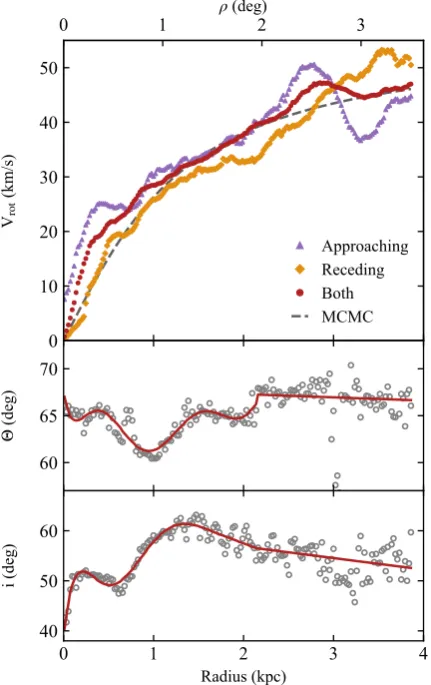
During the entire fitting procedure, we set the ring width to 35 arcsec, i.e. equal to the beam size of the observations and cor-responding to about 10 pc at the distance of the SMC. We use a cos (−) weighting function to give more importance to pixels near the kinematic major axis (i.e.=), which is where most of the information on the rotation velocity lies. We also exclude regions of the velocity field where−<20◦, i.e. close to the minor axis. After the first fitting step with rotation velocity, position angle, and inclination free, we regularizeiandwith a
seventh-degree polynomial function out toR=2 kpc and a straight line forR>2 kpc. The regularizing functions are chosen to best trace the overall trends of the angles. The middle and bottom panels of Fig.3show the solutions of the first fitting step for the position and inclination angles, respectively (grey empty circles) and their regularization (red lines). The position angle scatters between 60◦ and 70◦, with a median value very close to the 66◦found from the MCMC sampling. The inclination angle shows a larger variation in the range 40◦<i<60◦, with a median of 55◦slightly higher than the central value of the MCMC sampling.
Table 1. Global properties of the SMC disc, derived through the MCMC sampling described in Section 4.1.
Property Value
Assumed:
DistanceD0a 63±5 kpc
Proper motionμWb −0.772±0.063 mas yr−1
Proper motionμNb −1.117±0.061 mas yr−1
MCMC results:
RA of kinematic centreα0(J2000) 15.237+−0.3800.376deg
Dec. of kinematic centreδ0(J2000) −72.273+−0.2900.269deg
Inclination anglei 51±9 deg
Position angle of LONc 66±8 deg
Transverse velocityVtd 405±37 km s−1
Transverse directiontc,d 145±3 deg
Systemic velocityVsys(Heliocentric) 157±2 km s−1
Systemic velocityVsys(LSR) 148±2 km s−1
Precession/nutation∂i/∂t −281+−10288 deg Gyr−1
Asymptotic velocityVfe 56±5 km s−1
Turnover radiusRfe 1.1±0.2 kpc
aMedian and standard deviation from the literature (NED). bFrom Kallivayalil et al. (2013).
cMeasured anticlockwise from the north direction. dFrom proper motions andthrough equations (5). eFor the parametrized rotation curve of equation (6).
of the SMC disc. As a reference, we plot also the parametrized ro-tation curve (equation 6) resulting from the MCMC sampling (see Table1) as a grey dashed line. The global rotation curve slowly rises to a maximum velocity of∼47 km s−1atR∼2.8 kpc and appears to flatten at larger radii, although this flattening is not well defined. The maximum rotation velocity is slightly larger than the value found in Stanimirovi´c et al. (2004) (∼40 km s−1 and with a lower inclination angle) and older HIstudies (∼36 km s−1, e.g. Hindman1967; Loiseau & Bajaja1981). The differences between the rotation curves of the approaching and receding sides reflect the asymmetries of the velocity field. The three curves are quite consistent in the region 1 R 2.5 kpc, but they show larger discrepancies in the inner and outer parts. The latter might be due to the influence of the SMC wing and Magellanic Bridge on the receding side and of the SMC tail and Magellanic Stream on the approaching side.
Fig.4shows the velocity fieldVmodof the global best-fitting tilted-ring model (top panel) and the absolute residuals between model and observations, i.e.Vres= Vobs−Vmod(bottom panel). Despite the large asymmetries in the observed velocity field, our completely symmetric tilted-ring model does a fairly good job in reproducing the overall rotation behaviour of the SMC. The approaching half seems to be better reproduced than the receding half, which might be more affected by gas in motions to/from the Magellanic Bridge. Residuals in regions close to the major axis are of the order of a few km s−1. The largest residuals (∼20–25 km s−1) are found in regions with−20◦, i.e. near the minor axis, particularly in the east side. These areas are not used during the fit and the large discrepancies from our rotation model may indicate the presence of significant non-circular motions (see discussion in Section 7). The precession/nutation term∂i/∂talso causes a distortion of the velocity field that, according to the third term of equation (1), is more pronounced near the minor axis and at large angular distances from the galaxy centre. We therefore test the response of the minor axis residuals to different∂i/∂tby producing models varying with −600< ∂i/∂t<600 deg Gyr−1. Consistent with the values found
Figure 3. Tilted-ring analysis of SMC. Top: rotation curves derived after regularization of the inclination and position angles. Rotation curves of the approaching, receding, and both sides of the galaxy are shown with purple triangles, orange diamonds and red circles, respectively. The grey dashed line denotes the parametrized curve of equation (6) obtained through the MCMC sampling. Middle: variation of the position angle of the LON as a function of radius. Grey empty circles represent the first fitting step, the red line is the regularization used to derive the final rotation curve (see Section 4.2). Bottom: same as middle panel, but for the inclination angle. The ring width is 35 arcsec, i.e. about 10 pc at the distance of the SMC. in the MCMC sampling, we find that the more balanced residuals along the minor axis are for−300∂i/∂t−100 deg Gyr−1, while more positive/negative values cause larger residuals on one side or the other of the galaxy.
4.3 Asymmetric drift correction and SMC circular velocity
The circular velocityVc, i.e. the azimuthal component of the velocity induced in the equatorial plane by an axially symmetric gravitational potentialφ, can be written in terms of the average rotation of the gas Vrotin the disc plane plus the so-calledasymmetric driftcorrection VA:
Vc2(R)= −R
∂φ(R, z) ∂R
z=0
=Vrot2(R)+V 2
A(R) (8)
Figure 4. Best-fitting tilted ring model of the SMC disc. Top: model ve-locity field, using the same colour scale of the observed veve-locity field of Fig.1. Bottom: absolute residual map. Residuals are calculated only in the regions where both the observed and modelled velocity field are defined. Black crosses denote the best-fitting kinematic centre.
Carignan2002; Oh et al.2011):
VA2(R)= −Rσ 2 g
∂ln
σ2 ginth−z1
∂R = −Rσ 2 g
∂ln
σ2 gobscosi
∂R .
(9)
In the right-hand side of equation (9), we have made the assump-tion that the scale height is constant, so that we can ignore the radial derivative ofhz, and that the HIdisc is razor-thin, which implies int=obscosi, whereobsis the observed surface density. We also assume that the observed line broadening in each spectrum is a measure of the intrinsic velocity dispersion of the gas. We discuss the effect of these assumptions in detail in Section 7.
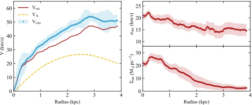
We use the surface density map (Fig.1, left) and the observed velocity dispersion field (Fig.1, right) to extractobs(R) andσg(R) profiles along the best-fitting rings found in Section 4.2. We take the median and the standard deviation of velocity dispersion and density in each ring as central values and associated errors. Right-hand panels of Fig.5show the derived surface density (bottom) and velocity dispersion (top) profiles. Similarly to many discs of star-forming galaxies, the HIsurface density follows an exponential profile with an inner core atR0.8 kpc. The velocity dispersion is quite high at all radii, ranging from about 20 km s−1in the central region and dropping to 15 km s−1in the outskirts. The H
Ivelocity
dispersion is therefore about half the rotation velocity. Assuming that such high values of dispersion are mainly due to turbulence in the SMC disc, then random motions provide a significant support to the system dynamics and the asymmetric drift correction cannot be neglected (however, see discussion in Section 7).
The radial derivative in equation (9) is very sensitive to fluctua-tions in the density and velocity dispersion profiles and it is good practice to regularize bothσg(R) and the argument of the logarithmic derivative with analytic functions to avoid meaningless discontinu-ities in the derived asymmetric drift correction. In our case, we regularize the velocity dispersion with a third-degree polynomial P3(R) and the argumentσ2
gobscosiwith a function characterized by an inner core followed by an exponential decline (see e.g. Iorio et al.2017):
f(R)=f0
Rc+1 Rc+exp(R/Rd)
(10)
wheref0is a normalization factor,Rcthe core radius, andRdthe scale radius for the exponential drop-off. With these approximations, equation (9) can be conveniently rewritten as
V2 A(R)=
RP2
3exp(R/Rd) Rd(Rc+exp(R/Rd))
. (11)
After regularizing the velocity dispersion andσ2
gobscosi, we compute the asymmetric drift correction through equation (11). We calculate the uncertainties on the final circular velocities by propa-gating the errors on the rotation velocity and the asymmetric drift based on equation (8). The uncertainty on the HIrotation veloc-ity is taken as the statistical error associated with the tilted-ring fit plus half of the difference between the rotation curves of the re-ceding and approaching halves. The latter term dominates the error budget in most cases. Following Iorio et al. (2017), we estimate the error on the asymmetric drift correction with a Monte Carlo approach: we produce 1000 realizations of the velocity dispersion σi
g(R) and intrinsic densityinti (R) profiles, where everyith realiza-tion is extracted from a normal distriburealiza-tion with mean and standard deviation given by the observed profiles. We then calculateVi
A(R) through equation (11) and take 1.48×MAD(Vi
A) as a measure of the asymmetric drift error, where MAD(Vi
A) is the median absolute de-viation about the median of all realizations. This procedure allows us to properly account for errors on the derived rotation velocity, velocity dispersion, and surface density in the final uncertainties on the derived circular velocity of SMC.
The left-hand panel of Fig.5shows the HIrotation curve derived for both galaxy halves (red full line), the asymmetric drift correction (yellow dashed line), and the resulting circular velocity through equation (8) (cyan dots). The shadowed region in Fig.5represents the uncertainties on the circular velocity formally propagated from the errors on the rotation velocity and asymmetric drift term. The correction for asymmetric drift causes an increase in the circular velocity of 7–10 km s−1between 1 R2.5 kpc and of about 5 km s−1 (∼10 per cent of the HIrotation velocity) in the outer regions. A machine-readable table with our final rotation curve is available as online Supporting Information.
5 M A S S D E C O M P O S I T I O N O F T H E S M C
In this section, we use the asymmetric-drift corrected rotation curve to construct mass models of the SMC. The observed circular velocity (equation 8) can be decomposed into the contribution of the different mass components (e.g. de Blok et al.2008) as
V2 obs=V
2 gas+ϒ∗V
2
Figure 5. Left: circular velocity of the SMC corrected for the asymmetric drift (cyan dots). Shadowed regions represent the 1σerrors, calculated as described in Section 4.3. The red curve identifies the HIrotation curve derived from both halves of the galaxy (same as Fig.3), and the yellow dashed line the asymmetric drift correction (equation 11). Right: velocity dispersion profile (top) and face-on HImass-density profile derived from the ASKAP data.
where Vgas, V∗, and VDM are the contribution of gas, stars and DM halo to the total rotation velocity. The stellar mass-to-light ratioϒ∗ rescales the contribution of the stellar component and
is needed because we measure the distribution of light rather than mass. In the following sections, we describe the density distributions that we use for the various mass components and the assumptions that we make. Unless an analytic solution exists, we numerically calculate the circular velocity in the planez=0 induced by any given density distribution integrating equation (8), where the potential φ(R,z) is computed using theGALPYNAMICSpackage (Iorio et al., in preparation).
5.1 Neutral gas distribution
We describe the mass surface-density distribution of the disc com-ponents (both stars and gas) with an exponential multiplied by a polynomial in the radial direction and a squared hyperbolic secant in the vertical direction:
d(R, z)= 0 2zd
Pn(R) exp
−R Rd
sech2
z zd
(13)
where0is the surface density in the centre,Pn(R) is ann-degree polynomial function,Rdis the disc scale length, andhzis the disc scale height. Note that equation (13) implies a constant scale height with radius, thus no flaring component is taken into account. In the case of a razor-thin pure exponential disc, i.e.zd=0 andPn=P0= 1, the circular velocity induced by the disc component is simply given by (Freeman1970):
Vd2(R)=4πG0Rdy2[I0(y)K0(y)−I1(y)K1(y)] (14)
whereGis the gravitational constant,y≡0.5R/Rd, andInandKn are modified Bessel functions ofnth kind. For the general case, the circular velocityVd(R) needs to be numerically integrated.
For the gas disc, we use a third-degree polynomial P3(R) to describe the observed inner depression in the gas distribution (see Fig.5, right). We correct the HIradial profile by a factor 1.4 to take into account the primordial abundance of helium and metals and fit it for0, gas,Rd, gas, andP3(R). We keep the scale heighthzas a free parameter and we build mass model using different scale heights (see Section 5.4).
5.2 Stellar distribution
We use two different model distributions for the stellar compo-nent: an exponential disc and an exponential prolate spheroid. The surface-density distribution of the former is described by equa-tion (13) withPn=1. We assume that gas and stellar discs always have the same scale height. The second model is meant to mimic the observed 3D structure of stars in the SMC. Several studies have used the period–luminosity relation of variable stars, in particular Classical Cepheids and RR Lyrae, to show that stars in the SMC are distributed in triaxial ellipsoids significantly elongated along the LOS (Deb et al.2015; Jacyszyn-Dobrzeniecka et al.2016,2017; Ripepi et al.2017). Here, we assume the axes ratio 1:1.10:3.30 quoted in the recent paper of Muraveva et al. (2018). Given the very small ratio of the first two axes, we approximate the triaxial shape with a prolate ellipsoid of axes ratio 1:1:3.30 and consider the exponential prolate spheroidal density distribution:
star(m)=pexp(−m/md) (15)
where, as usual,pis the central density andmdefines the isodensity surfacesm2=R2+z2/q2withq≡3.30 in our particular case. The quantitymdhas the meaning of a scale radius for the variablem.
We derive the observed stellar distribution from the mosaicked images at 3.6μm of the Surveying the Agents of a Galaxy’s Evolu-tion survey of the SMC (SAGE–SMC, Gordon et al.2011). SAGE– SMC is a survey of the full SMC system (main body, wing, and tail) covering about 30 deg2in seven bands from 3.6 to 160μm with the Infrared Array Camera (IRAC, Fazio et al.2004) and the Multiband Imaging Photometer (Rieke et al.2004) on theSpitzer Space Tele-scope(Werner et al.2004). At near-infrared (NIR) wavelengths, the light traces the old stellar populations and the effects of dust extinction and star formation (like HIIregions) are quite negligible compared to optical bands. Moreover, the mass-to-light ratioϒ∗in the NIR, in particular at 3.6μm, is almost constant over a wide range of galaxy morphologies (e.g. Bell & de Jong2001; Zibetti, Char-lot & Rix2009), reducing the uncertainties related to this unknown parameter. These characteristics make the 3.6μm light optimal to estimate the stellar mass distribution.
foreground emission in five regions nearby the SMC and subtract it from the profile. We finally convert from surface brightness to mass surface density following Oh et al. (2008):
∗
Mpc−2 =Cϒ 3.6
∗ cosi
I3.6
MJy sr−1 (16)
where ϒ3.6
∗ is the stellar mass-to-light ratio at 3.6μm and
C=696L sr MJy−1 pc−2. The constant comes from C= A/Z3.610[6+0.4(M
3.6
+21.56)], whereA = 2.35×10⁻¹¹ sr arcsec−2 is the number of steradians in one square arcsec,Z3.6=280.9 Jy is the IRAC zero magnitude flux density at 3.6μm (Reach et al.2005), andM3.6
=3.24 is the absolute magnitude of the Sun at 3.6μm
(see Oh et al.2008, for further details). We find that the 3.6μm surface-brightness profile is reasonably well described by a pure exponential function.
The mass-to-light ratioϒ∗constitutes the largest uncertainty in the conversion from stellar luminosity to mass (e.g. Ponomareva et al.2018) and this uncertainty reflects in any rotation curve de-composition. Several stellar population synthesis studies have found that the mass-to-light ratio at 3.6μm has little dependence on the population age and metallicity, thus on the colour (Meidt et al.
2014; Norris et al.2014). For example, for a Kroupa (2001) ini-tial mass function (IMF), the mass-to-light ratio varies between 0.4ϒ3.6
∗ 0.8 for stellar populations with ages between 3 and
10 Gyr (R¨ock et al.2015), i.e. by a factor of 2. Although this vari-ation is small compared to that in the optical (e.g. a factor of 10 within the same age range inVband, Vazdekis et al.2010), it can still introduce a significant uncertainty in the derived stellar mass. In addition, the absolute value ofϒ3.6
∗ is sensitive to the assumed
IMF (R¨ock et al.2015). A constantϒ3.6
∗ =0.5–0.6 is often
appro-priate for star-forming galaxies (e.g. Meidt et al.2014; McGaugh & Schombert2014). A very similar value,ϒ3.60.53, has been also found by Eskew, Zaritsky & Meidt (2012) for the LMC, based on spatially resolved star formation histories and a Salpeter (1955) IMF. To date, an analogue study on the SMC is still missing. In this contribution, we build models for several mass-to-light ratios (see Section 5.4).
5.3 Dark matter haloes
We consider two different spherical models for the DM distribution. The first model is a pseudo-isothermal halo, which has a density profile given by:
iso(r)=0
1+
r rc
2 −1
(17)
whereris the spherical radius,0is the central density, andrcis the core radius of the halo. This model is characterized by a central constant-density core and a quadratic decline for radii larger thanrc. The contribution to the circular velocity due to the density profile in equation (17) is
V2
iso(R)=4πG0rC2
1−rc Rarctan R rc . (18)
The second model is a halo with a Navarro–Frenk–White (NFW, Navarro, Frenk & White1996,1997) density profile:
NFW(r)=c
r rs
1+ r
rs 2 −1
(19)
wherersis a scale radius of the halo andc=critδc, beingcritthe critical density of the Universe, andδca dimensionless characteristic
contrast density. The NFW profile arises fromN-body simulations of structure formation in a cold dark matter (CDM) cosmology and is characterized by a central density cusp (NFW∼r−1forrrs). As for the pseudo-isothermal case, the rotation velocity in the plane of the disc induced by an NFW halo can be written in analytic form as:
VNFW2 (R)=V 2 200
ln(1+cx)−cx/(1+cx)
x[ln(1+c)−c/(1+c)] (20)
wherex=R/R200,V200is the rotation velocity atR200, the radius inside which the average density is 200 times the critical density of the Universe, roughly corresponding to the virial radius, andc= R200/Rsis the halo concentration. The parameterscandV200can be then related to density profile parameterscandrs(see Navarro et al.1996).
5.4 Mass models
We use the observed rotation curve and the derived stellar and gas circular velocities to least-squares fit the parameters of the DM halo through equation (12). Given the uncertainties on the actual 3D shape of the SMC, we explore a range of interesting cases by varying the properties of both the baryonic and non-baryonic matters. In particular, we vary the thickness of the disc components in the range 0≤hz≤1 kpc, the mass-to-light ratio between 0.2≤ ϒ3.6
∗ ≤1, chosen to take into account the wide range of values
predicted by stellar population synthesis models (e.g. R¨ock et al.
2015), and we use either a disc or a prolate spheroid for the stellar component. We build models with and without DM: in the first case, we assume either a pseudo-isothermal (cored) or an NFW (cusped) halo and fit their properties to the observed rotation curve, in the second case, we let the stellar component supply all the mass needed to reproduce the rotation curve by leaving free the mass-to-light ratioϒ3.6
∗ .
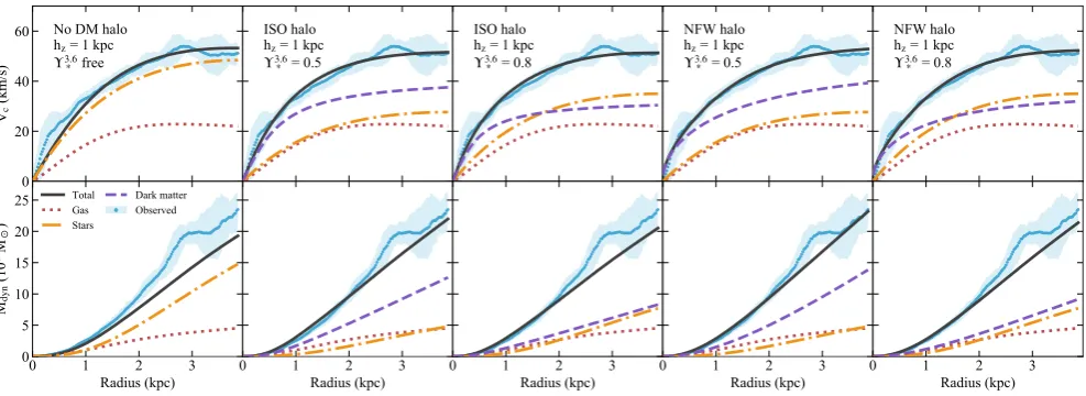
Figs6and7show mass models with a stellar disc and a stellar prolate ellipsoid, respectively, and a thick disc component hz = 1 kpc. Models with a thin disc (hz ∼ 0 kpc) are not shown as they provide a poorer fit to the data. In both figures, the first row represents the rotation curve decomposition, the second row denotes the corresponding cumulative masses for stars (dotted– dashed yellow line), gas (red dotted), and DM (dashed purple), calculated by integrating the best-fitting density profiles. The ob-served rotation curve and enclosed mass for a spherical distribution Mobs(< R)=RV2
obs(R)/Gare shown as blue dots, with shadowed regions representing the errors. Black solid lines are the total mod-elled rotation curve and cumulative mass. Starting from the left, we plot models with no DM, pseudo-isothermal, and NFW DM haloes with fixedϒ3.6
∗ =0.5 and 0.8. Most models provide good
fits to the observed circular velocity. However, models with no DM (first column) lead to very high mass-to-light ratios (ϒ3.6
∗ 1.5)
and stellar masses (M∗>109M
), which make them unlikely. A DM matter halo is needed for all models with sensibleϒ3.6
∗ . In
par-ticular, for ϒ3.6
∗ <0.7, the DM component always dominates the
overall mass budget at all radii. The total needed DM mass within 4 kpc is of the order of 1–1.5×10⁹M
depending on the assumed
Figure 6. Mass models for the SMC with a thick disc stellar and gas components (hz=1 kpc). Models with different DM haloes (no DM, pseudo-isothermal,
and NFW) and 3.6μm mass-to-light ratios are represented. Top row shows the rotation curve fits for each model, and bottom row is the correspondent total mass within a radiusR. The contributions of stars, gas, and DM are shown as yellow dotted–dashed, red dotted, and purple dashed lines, respectively. The total model is the black thick line. Cyan dots represent the observed quantities, with the shadowed areas being the 1σerrors. Mass models with no DM (first column) are highly unlikely as they lead to unreasonableϒ3.6
∗ .
Figure 7. Same as Fig.6, but for mass models with a thick gas disc (hz=1 kpc) and a prolate stellar spheroid with axis ratioq=3.30 (see equation 15). Our
best model is with an NFW halo and a stellar mass-to-light ratioϒ3.6
∗ =0.5 (fourth column from the left).
(Fig.7) lead to similar mass decompositions and to rotation curves that differ by just a few km s−1, being equal the total enclosed stellar mass.
The best mass model (i.e. lowestχ2) is achieved with the ellip-soidal stellar distribution, a thick gas disc distribution (hz=1 kpc), an NFW DM halo, andϒ3.6
∗ =0.5 (fourth column in Fig.7). The
best-fitting DM halo has a central densityc=5.2×10⁶Mkpc−3
and a scale radiusrs=5.7 kpc. This model nicely reproduces the observed rotation curve and well traces the cumulative mass except for the bump at around 3 kpc. A mass-to-light ratioϒ3.6
∗ =0.5 is
consistent with stellar population models (Meidt et al.2014; Mc-Gaugh & Schombert2014) and estimates in the LMC (Eskew et al.
2012). This implies a stellar massM∗∼4.8×10⁸M
withinR
4 kpc, slightly higher but comparable with the total estimated stellar mass of the SMC (3–3.5×10⁸M
, e.g. Harris & Zaritsky
2004; Skibba et al.2012). The total mass of neutral gas (HI +He
+metals) within the same radius isMgas∼4.7×10⁸M, of which
MHI∼3.4×10⁸M is atomic hydrogen (see also Stanimirovi´c
et al.1999). A dominant DM halo with massMDM∼1.4×10⁹M
is therefore needed to justify a total inferred dynamical mass of Mtot2.4×109M(bottom row of Fig.7). The dynamical mass
found in this work is consistent with the one quoted in Stanimirovi´c et al. (2004) but smaller than the value of 2.7–5.1×10⁹M
in-dependently estimated by Harris & Zaritsky (2006) based on the velocity dispersion of stars. In our best-fitting model, the baryon fraction of the SMC is thereforefbar∼40 per cent, a large value compared to other dwarf galaxies in the local Universe (e.g. Oh et al.2015). The strong concentration of baryons may indicate that the SMC accreted some gas and stars during the current interaction with the LMC or during a past major merger event (Bekki & Chiba
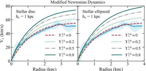
[image:11.595.50.544.314.494.2]Figure 8. Decomposition of the SMC rotation curve in a MOND frame-work, using a stellar disc (left) or a stellar prolate ellipsoid (right). The curves denote the MOND predictions for different mass-to-light ratiosϒ3.6
∗ , as indicated in the legend. MOND overpredicts the circular velocity of the SMC forϒ∗3.6>0.
5.5 Mass models in Modified Newtonian dynamics
Modified Newtonian dynamics (MOND, Milgrom1983; Sanders & McGaugh2002, for a review) is often seen as an alternative to DM to explain the discrepancy between theoretical baryon-only and observed rotation curves of galaxies (e.g. de Blok & McGaugh
1998; Swaters, Sanders & McGaugh2010; Randriamampandry & Carignan2014). In this section, we decompose the SMC rotation curve using the MOND paradigm and investigate whether MOND can reproduce the observed kinematics of the dwarf galaxy without the need of a DM halo.
Within the MOND framework, the equivalent of equation (12) for the circular velocity can be written as (e.g. Gentile2008):
VMOND2 =V 2 bar+V
2 bar
1+4a0r/Vbar2 −1 2
(21)
whereV2
bar=Vgas2 +ϒ∗V∗2is the Newtonian contribution to the
cir-cular velocity of baryonic matter (stars +gas) anda0is the critical acceleration below which the MOND regime dominates and the Newtonian gravity is no longer valid. The second term of equa-tion (21), which is entirely set by the baryonic matter and vanishes fora0→ 0, replaces the DM halo in Newtonian dynamics. We stress that equation (21) is only valid for an interpolation func-tionμ(x)=x(1+x)−1withx≡g/a
0andg=V2/r, as proposed by Famaey & Binney (2005). In this work, we assume the value a0=1.35×10⁻⁸cm s−2=4166 km2s−2kpc−1found by Famaey et al. (2007) for the above interpolation function.
We least-squares fit equation (21) to the observed circular veloc-ity curve of the SMC. The velocveloc-ity contributions of gas (Vgas) and stars (V∗) are calculated as in the Newtonian case using the mass profiles described in Sections 5.1 and 5.2, respectively. Sincea0is a universal constant in MOND, we perform the fit with only the mass-to-light ratioϒ3.6
∗ as a free parameter. Independently from the
disc scale height and for either a stellar disc or a stellar ellipsoid, the best fit is achieved for aϒ3.6
∗ =0, i.e. nullifying the contribution of
the stars to the rotation curve. This solution is undoubtedly unphys-ical and implies that, in a MOND framework, the mass of gas alone is enough to justify the rotation velocity. Assuming a non-nullϒ3.6
∗
leads to overestimate the circular velocity at all radii. This is clearly shown in Fig.8, where we plot MOND rotation curves for various ϒ3.6
∗ , for both a stellar disc (left-hand panel) and a prolate ellipsoid
(right-hand panel) and with a scale heighthz=1 kpc. We conclude that the dynamics of the SMC cannot be explained in MOND as the galaxy is too rich in baryonic matter, causing MOND to
systemat-ically overpredict the circular speed curve for any non-null stellar mass-to-light ratios.
6 C O M PA R I S O N W I T H OT H E R S T U D I E S
The HIkinematics and dynamics of the SMC have been previously investigated in the papers of Stanimirovi´c et al. (2004) and Bekki & Stanimirovi´c (2009). Both those works made use of the same HIdata set obtained from ATCA observations (Staveley-Smith et al.1997) combined with single-dish data from the 64-m Parkes telescope (Stanimirovi´c et al.1999). These data have a smaller sky coverage (20 versus 45 deg2) and velocity coverage (130 versus 510 km s−1), a coarser spatial resolution (98 arcsec versus 35 arcsec) and less sensitivity (1.3 versus 0.7 K) than our ASKAP data, but a finer spectral resolution (1.65 versus 3.90 km s−1).
Stanimirovi´c et al. (2004) use a proper-motion-corrected velocity field to derive the rotation curve of the SMC with a classic tilted-ring model, including an asymmetric drift correction. We note that they decided to use only the Parkes HIdata as the ATCA+Parkes data were too complex. Compared to their approach, we start from updated proper motions and distance (Table1), we use spherical ge-ometry to take into account the velocity field distortions due to the angular size of the SMC (Section 3) and we follow a two-step fitting procedure to separately estimate the global kinematic/geometrical parameters (Section 4.1) and the rotation curve (Section 4.2). Sta-nimirovi´c et al. find geometrical parameters that differ from ours, in particular the kinematic centre, position, and inclination angles, which results in slightly different shapes of the observed rotation curves. Their maximum observed velocity, i.e. before the correction for asymmetric drift, is however similar to the one derived in this work. After the asymmetric drift correction, the circular velocity from Stanimirovi´c et al. reaches a maximum of 60 km s−1, a value larger than ours (∼55 km s−1
), but consistent within the respective errors. They decompose the rotation curve with a two-component (gas +star discs) mass model and concluded that no DM halo is needed to explain the observed velocities. Their model however im-plies an excessively large stellar massM∗=1.8×10⁹Mwithin
R=3.5 kpc, which conflicts with recent estimates (Skibba et al.
2012).
Bekki & Stanimirovi´c (2009) reanalyse the rotation curve from Stanimirovi´c et al. (2004) to investigate the possible contribution of a DM halo within the central 3 kpc. They useV-band images to trace the stellar component, they adopt a smaller total stellar luminosity than Stanimirovi´c et al. (2004) and model the observed rotation curve with a thick disc stellar and gas components and a DM halo following either an NFW or a Burkert (1995) density profile. We note that the usage ofV-band images to derive the stellar contribution to the total rotation curve introduces a significant uncertainty due to the large variations of the mass-to-light ratio in the optical. They none the less end up with DM halo masses of the order of 1–1.5×10⁹M
for reasonableϒV
∗ within 3 kpc, in good
agreement with our best-fitting value. Different from our analysis, they point out that a Burkert DM profile with a large core reproduces the observed rotation curve better than a cusped NFW halo. This is likely due to the fact that our rotation curve rises more steeply than that in Stanimirovi´c et al. (2004) in the inner 0.5 kpc and therefore DM profiles with a central cusp are favoured over profiles with a central core.
the Magellanic system (van der Marel & Sahlmann2016; Gaia Col-laboration et al.2018).Gaiaresults confirm that stars and gas in the SMC do not share common kinematics. While the gas appears to be settled in a disc with a fairly well-defined rotation curve, the stars do not show a strong and coherent velocity gradient across the galaxy and several kinematic systems with very different dynamical histo-ries likely co-exist depending on the stellar population. Although proper motions suggest some sense of rotation (certainly less than HI), attempts to derive a stellar rotation curve are also hindered by the complex and uncertain geometry (Gaia Collaboration et al.
2018).Gaiatogether with previous optical surveys will allow us to better determine how the various stellar systems trace the effects of interaction between the MCs as well as past episodes of enhanced star formation. Given the complexity of the stellar components, the HIgas is probably the best tracer of the gravitational potential of the SMC, being sufficiently widespread and dynamically relaxed. Finally, we note that the global proper motions of the SMC de-termined withGaiaare quite similar to and statistically consistent with the values from Kallivayalil et al. (2013) values used in our analysis. As we discussed in Section 4.1, slightly different values ofμN and μWdo not strongly affect our derived kinematics, as the errors on the rotation curve are dominated by the asymmetries between the receding and approaching side and by the inclination uncertainties.
7 C AV E AT S
Our analysis is based on several techniques widely used in the litera-ture to derive the kinematics of external galaxies from emission-line observations. In particular, the tilted-ring model (Section 4.2) and the correction for asymmetric drift (Section 4.3) are commonly ap-plied to both disc galaxies (e.g. Begeman1987; de Blok et al.2008) and dwarf galaxies (e.g. Swaters1999; Oh et al.2015). A tilted-ring model relies on the assumption that gas moves in perfectly circular orbits about the galaxy centre. Moreover, when the model is ap-plied to a 2D velocity field, the disc is presumed to be infinitely thin. Although these assumptions are well suited for spiral galaxies, they can be inappropriate for dwarf galaxies like the MCs, where the shallow gravitational potential causes the disc to be quite thick, especially in the outer regions (Roychowdhury et al.2010), and non-circular motions can be a non-negligible fraction of the rota-tion velocity. In the case of the SMC, the tidal interacrota-tions with the LMC and the MW add a further source of uncertainty. Although accounting for all these effects is virtually impossible, it is useful to discuss these approximations and the impact they might have on the results presented in this paper.
The thin disc assumption allows us to easily translate between observed and intrinsic properties of a galaxy: (i) the values on the 2D velocity field directly measure the rotation motions in the equatorial plane, (ii) the face-on surface density can be calculated by simply correcting the observed density profile for the inclination angle, and (iii) the observed velocity dispersion is a measure of the intrinsic turbulent motions. In the presence of a thick gaseous disc, these properties do not hold and the derived kinematics may not reflect the true kinematics of the galaxy. We stress that 2D methods based on the velocity maps, like the ones used in this work, cannot handle a thick disc. The 3D techniques (J´ozsa et al.2007; Di Teodoro & Fraternali2015) guarantee a better treatment of the disc scale height, but they are computationally expensive and cannot be applied to our large ASKAP data. However, the effects of approximating a thick with a thin disc are known (e.g. Iorio et al.2017): (i) the derived rotation velocity at small (large) radii is lower (higher) than the
real rotation velocity, (ii) the observed density profile is shallower than the true profile, and (iii) the measured velocity dispersion overestimates the real turbulent motions. The first point affects the derived shape of the rotation curve, the last two points lower the correction for the asymmetric drift (equation 9). In summary, a thick disc causes the circular velocity in the outer regions to be overestimated, which results in the overestimation of the total dynamical mass and, consequently, of the mass of the DM halo. In this context, our estimated DM mass ofMDM1.4×109M
should be read as an upper limit.
The second big limitation of our modelling is the assumption of pure circular motions. Although the SMC velocity field (Fig.1) shows some clear regularity, it is far from being the classical velocity field of a simply rotating galaxy. The effect of regular non-circular velocity components, like streaming motions for instance, usually shows up as a twist in the iso-velocity contours, more evident on the minor axis. The regions close to the minor axis of the SMC velocity field significantly deviate from regular rotation, suggest-ing the presence of substantial non-circular motions. One could in theory modify equation (1) to take into account additional ve-locity components, like radial and/or vertical motions, however this would lead to further degeneracies that would be difficult to control. Moreover, the velocity residuals (Fig.4) show no regular pattern, suggesting that non-circular motions in the SMC are likely dom-inated by the tidal interaction with the LMC/MW and cannot be easily described with additional velocity terms. We tried to reduce the impact of non-circular motions by applying a weighting function and masking disturbed regions of the velocity field, it is however difficult to quantify their net effect on the derivation of the rotation curve. A secondary consequence of chaotic non-circular motions is the broadening of the line profiles, which results in the turbu-lent velocity dispersion being overestimated. This couples with the analogous effect of the disc thickness and leads to an overcorrec-tion for the asymmetric drift and a circular velocity larger than the real one.
Finally, a potentially important source of errors is the inclination angle, which is very uncertain for the SMC. The estimate of the true inclination angle from HIdata is hampered by the complex morphology of the SMC and its unknown geometry (for example, a thick disc would cause the inclination angle to be underestimated). Independent determinations of the inclination for the putative stellar disc are even more problematic, with values ranging from 5◦to 70◦ depending also on the probed stellar population (e.g. de Vaucouleurs
1955; Subramanian & Subramaniam2012; Haschke et al.2012). In this work, we obtain an inclinationi=(51±9)◦from the MCMC sampling and an averagei =55◦from the tilted-ring model for the HIdisc. These values are quite a bit larger than the 40◦previously found by Stanimirovi´c et al. (2004). Although our HIdata seem to discourage very low inclination angles, in our modelling we still have uncertainties of the order of 10◦. Since the measured rotation velocity scales as (sini)−1, an inclination 10◦lower would lead to a larger maximum circular velocity of∼64 km s−1and a larger dynamical mass∼3.2×10⁹M
. On the other end, an inclination
10◦ higher would translate into a smaller maximum velocity of ∼50 km s−1and a smaller dynamical mass∼2×10⁹M
.
8 S U M M A RY A N D F I N A L R E M A R K S