MoL 2019 08: Polyhedral Completeness in Intermediate and Modal Logics

(1)

Polyhedral Completeness in Intermediate and Modal Logics

MSc Thesis

(Afstudeerscriptie)

written by

Sam Adam-Day

(born 15th September, 1993 in Bath, United Kingdom)

under the supervision ofDr. Nick Bezhanishvili, and submitted to the Board of Examiners in partial fulfillment of the requirements for the degree of

MSc in Logic

at theUniversiteit van Amsterdam.

Date of the public defense: Members of the Thesis Committee:

2nd July, 2019 Dr. Alexandru Baltag Prof. Johan van Benthem

(2)

Abstract

This thesis explores a newly-defined polyhedral semantics for intuitionistic and modal logics. Formulas are interpreted inside the Heyting algebra of open subpolyhedra of a polyhedron, and the modal algebra of arbitrary subpolyhedra with the topological interior operator. This semantics enjoys a Tarski-style completeness result:IPCandS4.Grzare complete with respect to the class of all polyhedra. In this thesis I explore the general phenomenon of completeness with respect to some class of polyhedra.

I present a criterion for the polyhedral completeness of a logic based on Alexandrov’s nerveconstruction. I then use this criterion to exhibit an infinite class of polyhedrally-complete logics of each finite height, as well as demonstrating the polyhedral polyhedrally-completeness of Scott’s logicSL. Taking a different approach, I provide an axiomatisation for the logic of all convex polyhedra of each dimensionn.

(3)

Acknowledgements

I owe a debt of gratitude to many people. Chiefly, Nick: thank you for your endless draft-reading, your stimulating meetings and your belief in me. This thesis would be impossible without you.

David and Enzo: your collaboration and support have been essential to me throughout the whole process. It has been a pleasure to work with you and Nick, and I hope that we can continue to collaborate on this and other projects in the years to come. I wish to especially thank David, who greatly helped me in refining and simplifying the proof of convex completeness in Chapter 4.

Helen, Ken and BB, who have supported me throughout my life: thank you. I am very grateful to Helen, who is always happy to meticulously proof-read anything I write.

My friends Mina, Rachael, Dean, Zhuoye, and so many more incredible people on the Master of Logic: thank you for your friendship and for making my years at the ILLC the most special time of my life.

(5)

Chapter 0

Introduction

Let no one ignorant of geometry enter here

According to legend, inscribed above the door to Plato’s Academy

Geometry and logic share a long friendship. Mathematical logic in the West probably first found its feet in connection with the emergence of geometry as ana prioridiscipline [KK62]. The Ancient Greeks inherited a collection of empirically-verified geometric observations from the Egyptians and Babylonians, and it was their great achievement to systematise the study and place it on a solid logical basis, culminating in Euclid’s celebratedElements.

It is only relatively recently, however, that a deeper connection between geometry and logic has started to emerge. Multiple lines of research have explored links with diverse areas, from type theory to model theory. In this thesis I contribute to a line of research which seeks to traverse another fibre of this connection, by relating intuitionistic and modal logic with algebras of polyhedra. In order to warm up, and to provide some context for the present investigation, let us take a brief tour of a selection of already-established logic-geometry links. This is by no means a comprehensive overview, but I hope that these examples serve to give a flavour of the situation as it stands today. Numerous other examples can be found in the Handbook of Spatial Logics[APB07], which provides an excellent survey of some of the recent developments in this area.

Perhaps the most direct link between logic and geometry can be found in Alfred Tarski’s seminal work investigating the logical foundations of geometry, following David Hilbert’s programme of rigorously founding Euclid’s work[Hil50]. In[Tar59], Tarski shows how all ofelementary geometry— “that part of Euclidean geometry which can be formulated and established without the help of any set-theoretical devices” — can be formalised in first-order logic using only the notions ofbetweennessandequidistanceas non-logical concepts. He demonstrates that such a system is decidable, but not finitely axiomatisable. This work was further developed by Tarski and his followers, looking for instance at non-Euclidean geometries. More recently, fragments of elementary geometry have been formalised using modal logic, by interpreting the modaland◇in interesting

(6)

Another fibre of the logic-geometry link istopos theory. Alexander Grothendieck invented toposes as a generalisation of topological spaces, to deal with the numerous situations occurring in mathematics which involve topology-like and continuity-like arguments, but where a genuine topological space is absent[Vic07]. Grothendieck’s toposes play an important role in algebraic geometry, but topos theory also has close connections to logic via the more general notion of anelementary topos. The situation is summed up succinctly by Saunders MacLane and Ieke Moerdijk, who begin their prologue to[MM94]as follows.

A startling aspect of topos theory is that it unifies two seemingly wholly distinct mathematical subjects: on the one hand, topology and algebraic geometry, and on the other hand, logic and set theory. Indeed, a topos can be considered both as a “generalized space” and as a “generalized universe of sets”.

As a somewhat related example, consider the relation, discovered around the turn of the 21st_{century, between Martin-Löf type theory and homotopy theory. The former is a} theory of types originally intended for use as a foundation for constructive mathematics. Its pertinent feature is that it accommodates two kinds of equality: the usualdefinitional equality, and a (new)propositionalequality. Propositional equality between objectsaand bamounts to theidentity type, Id(a,b), being inhabited. Objects of type Id(a,b)can be thought of both as proofs of the equality ofaandb, and as ‘paths’ fromatob. But for any two suchp,qin Id(a,b), one may formtheiridentity type Id(p,q). Ifpandqare thought of as paths fromatob, then the objects of Id(p,q)should be thought of as homotopies between pandq. And this scheme continues to higher levels. This culminates in an elegant relationship between type theory and (higher) homotopy theory, which allows the two-way transfer of ideas. Indeed, Steve Awodey begins his[Awo10]on the subject as follows.

The purpose of this informal survey article is to introduce the reader to a new and surprising connection between Geometry, Algebra, and Logic, which has recently come to light in the form of an interpretation of the constructive type theory of Per Martin-Löf into homotopy theory, resulting in new examples of certain algebraic structures which are important in topology.

(7)

McKinsey and Tarski showed[MT44]that for any separable metric space X without isolated points, ifIPC0φ, thenφhas a countermodel based onX, and similarly withS4 in place ofIPC. Later, this result was refined still further by Helena Rasiowa and Roman Sikorski, who showed that one can do without the assumption of separability[RS63].

This result traces out an elegant interplay between topology and logic; however, it simultaneously establishes limits on the power of this kind of interpretation. Indeed, examples of separable metric spaces without isolated points are then-dimensional Eu-clidean spaceRnand the Cantor space 2ω. What McKinsey and Tarski’s result shows is that — topologically speaking — the logics of these spaces are the same, namelyIPCor S4. The upshot is that topological semantics does not allow logic to capture much of the geometric content of a space.

A natural idea is that, if we want to remedy the situation and allow for the capture of more information about a space, then we need a more fine-grained algebra than the Heyting algebra of open sets, or the modal algebra of arbitrary subsets with the interior operator. This idea was developed by Marco Aiello, Johan van Benthem, Guram Bezhanishvili and Mai Gehrke. They consider the modal logic ofchequeredsubsets of Rn: finite unions of sets of the formQni=1Ci, where eachCi⊆Ris convex ([ABB03]and [BBG03]; see also[BB07]).

In this thesis, I pick up a line of research, initiated by[BMMP18]and further inves-tigated in[Gab+18], which takes this algebra-refinement idea one step further. Since our aim is to be able to capture some of the geometric content of a space, it is natural to restrict attention to topological spaces and subsets which arepolyhedra(of arbitrary dimension). It turns out that this works: after making this restriction, one finds oneself in an environment which is still logic-friendly. That is, the set Subo(P)of open subpolyhedra ofPis a Heyting algebra under⊆(and a similar result holds in the modal case). The main result of[BMMP18]is that more is true. A polyhedral analogue of Tarski’s theorem holds: these polyhedral semantics are complete forIPCandS4.Grz. Furthermore, this approach delivers at least some of what we wanted: logic can capture the dimension of the polyhedron in which it is interpreted, via the bounded depth schema.

Two lines of approach. The Main Question driving the investigation in this thesis is the following. Which other geometric properties of polyhedra can be captured under these polyhedral semantics? Another way of putting this is: which logics are complete with respect to some class of polyhedra? In fact, these two dual expressions exemplify the two ways in which we will approach the problem. Starting with a classCof polyhedra (say, specified by a certain geometric property), one can ask: what is the logic ofC? This is the approach taken in Chapter 4, where we consider the logic of the class of convex polyhedra in each dimension.

(8)

Outline and main results. In Chapter 1, I remind the reader of the key logical machinery which will be active in this thesis, and cover the basic parts of polyhedral geometry which we will need. I then unite these two areas by showing that the set Sub_o(P)of open subpolyhedra of a polyhedronPforms a locally-finite Heyting algebra, following[BMMP18].

This unison is deepened in Chapter 2. I define the nerveN(F)of a poset F, and give two ways in which it is used to relate logic with polyhedral geometry. (1) The nerve enables the geometric realisation of F: there is a polyhedronP which maps in an appropriate way onto F. This then yields the final piece in the proof, following [BMMP18], that polyhedral semantics is complete forIPC. (2) The nerve construction is closely related to the operation ofbarycentric subdivisionon a triangulation. Exploiting this relation I present a proof — from joint work with Nick Bezhanishvili, David Gabelaia and Vincenzo Marra — of theNerve Criterion for polyhedral completeness: a logic Lis complete with respect to some class of polyhedra if and only if it is the logic of a class of finite frames closed under taking nerves. Viewing this result in terms of Kripke frames, we can say that “the logic of a polyhedron is the logic of the iterated nerves of any one of its triangulations”. The criterion yields many negative results, showing in particular that there are continuum-many non-polyhedrally-complete logics with the finite model property.

At this point, the only logics known to be polyhedrally-complete are, speaking in-tuitionistically,IPCand the logicBDnof bounded depthn, for each n. In Chapter 3, I expand the known domain of polyhedrally-complete logics, following the logical approach mentioned above. I consider logics defined usingstarlike treesasforbidden configurations — i.e. logics defined by theJankov-Fine formulasof a collection of trees with a special property: trees which only branch at the root. Exploiting the Nerve Criterion, I prove that every such logic is polyhedrally-complete if and only if it has the finite model property. This yields an infinite class of polyhedrally-complete logics of each finite height, as well as one of infinite height: Scott’s logicSL. As forbidden configurations, starlike trees turn out to have a clear geometric meaning, expressing connectedness properties of polyhedral spaces, and this provides one answer to the Main Question. One might wonder if a generalisation is possible to arbitrary trees, or even to a wider class of frames. As to the latter, some negative results are known; see Corollary 4.12. For the former, the situation is rather obscure, and it is not clear whether it is possible to account for the additional complexity introduced by allowing branching at higher points of the tree; see the discussion on ‘general trees’ in Section 3.4.

(9)

[image:9.595.216.380.118.202.2]

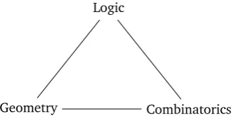
Geometry Combinatorics Logic

Figure 1: The triad of fields

(10)

Chapter 1

Background and Set-up

In this chapter, I go over the needed background from logic and geometry, and set up the first link between them. Throughout, I will assume familiarity with basic topology and linear algebra. I will also assume knowledge of elementary notions from category theory, such asfunctor,equivalenceandduality. For a clear introduction to these concepts I refer the reader to[Awo06], but this knowledge is not essential for most of the thesis.

1.1 Logical Machinery

The main kind of logic considered in this thesis isintuitionistic logic. In this section I remind the reader of the main definitions and results which we will need later on, and also set up some notation, primarily following[CZ97]. Another kind of logic, namely modal logic, is also important. However, as we shall see, results in the present setting transfer freely between intuitionistic logic and modal logic, and it suffices to consider only one of the two. I opt for the former, in line with[BMMP18].

Intermediate logics. We begin with a set Prop of propositional variables, and generate the setFormof formulas in the usual way, using the connectives⊥,∧,∨and→. Alogic_L is a deductively-closed set of formulas. WriteL `φforφ∈ L. The logicIPC is the standard intuitionistic propositional logic. Anintermediate logicis a consistent logic extendingIPC. Classical propositional logic,CPC, is the largest intermediate logic. I will usually use the term ‘logic’ as a shorthand for ‘intermediate logic’. The actual gory syntax of the logics plays a rather ancillary role in this thesis, and we will mainly be concerned with its semantic aspects. I will outline here two standard types of structure in which intermediate logics are interpreted.

Posets as Kripke frames. AKripke framefor intuitionistic logic is simply a poset

(F,¶). For technical reasons, let us allow∅as a frame. The relationis defined in the usual way. Given a class of framesC, itslogicis:

Logic(C):₌{φ∈Form| ∀F ∈C:F φ} Conversely, given a logicL, define:

(11)

A logicL has thefinite model property(f.m.p.) if it is the logic of a class of finite frames. Equivalently, ifL =Logic(Frames_fin(L)).

PROPOSITION1.1. (1) IPCis the logic of the class of all frames.

(2) IPChas the finite model property, so thatIPCis the logic of the class of all finite frames.

Proof. See[CZ97, Theorem 2.43, p. 45 and Theorem 2.57, p. 49].

The structure of Kripke frames. Let us carve out some additional vocabulary and notation. Fix posetsFandG. AsubframeofF is a subsetH_⊆F regarded as a subposet. For anyx_∈F, itsupset,downset,strict upsetandstrict downsetare defined, respectively, as follows.

↑(x):₌_{y_∈F_|y¾x}

↓(x):={y∈F|y¶x}

⇑(x):₌{y∈F|y>x} ⇓(x):₌_{y∈F|y<x}

For any setS⊆F, itsupsetanddownsetare defined, respectively, as follows.

↑U:₌ [ x∈U

↑(x)

↓U:₌ [ x∈U

↓(x)

A subframeU_⊆F isupwards-closedor agenerated subframeifU=_↑U. It is downwards-closedif↓U=U. TheAlexandrov topologyonFis the set of its upwards-closed subsets. This constitutes a topology onF. In the sequel, we will freely switch between thinking ofF as a poset and as a topological space. Note that the closed sets in this topology correspond to downwards-closed sets.

Atop elementofF ist∈F such thatdepth(t) =0. The set of top elements in F is denoted byTop₍F); letTrunk₍F):₌F\Top₍F). Thetop widthofFis|Top₍F)|. For any x,y∈F, say thatxis animmediate predecessorof yand thatyis animmediate successor ofx ifx<yand there is noz∈F such thatx<z< y. Write Succ(x)for the collection of immediate successors ofx.

AchaininF isX⊆Fwhich as a subposet is linearly-ordered. Thelengthof the chain X is|X|. The chainXisstrictif there are nox<y<zsuch thatx,z∈X but y∈/X. Take any subframeH_⊆F. A chainX_⊆His maximal (inH) if there is no chainY_⊆Hsuch thatX_⊂Y (i.e. such thatX is a proper subset ofY). TheheightofH is the element of N∪ {∞}defined by:

height(H):₌sup{|X| −1|X⊆His a chain}

For notational uniformity, say that this value is also thedepth ofH, depth(H). Let height(∅) =depth(∅) =−1. Note that these definitions apply whenH =F. For any x∈F, define itsheightanddepthas follows.

height(x):=height(↓(x)) depth(x):₌depth(↑(x)) Theheightof a logicL is the element ofN∪ {∞}given by:

(12)

A frameF hasuniform height nif every top element has heightn.

The poset F isrootedif it has a minimum element, which is called theroot, and is usually denoted by⊥. Define:

Frames_⊥(L):₌{F ∈Frames(L)|F is rooted}

Frames_⊥,fin(L):={F ∈Framesfin(L)|F is rooted}

PROPOSITION1.2. Frames_⊥₍CPC_{) =}{•}, the singleton of the 1-element poset. Proof. Note that ifFp∨ ¬pandF is rooted thenF=•.

Thecomparability relation./onF is defined:

x./y ⇔ (x<yor y<x)

Say that xand yarecomparableifx ./ y. Thecomparability graphofF is the graph

(F,./). ApathinF is a path in its comparability graph — in other words, a sequence p=x₀_{· · ·}x_kof elements ofF such that for eachiwe havex_i./x_i₊₁. Writep:x₀x_k. The pathpis closed ifx₀=x_k. The posetF ispath-connectedif between any two points there is a path.

PROPOSITION1.3. WhenFis finite, it is path-connected if and only if it is connected as a topological space.

Proof. See[BG11, Lemma 3.4].

Aconnected componentofF is a subframe U_⊆ F which is connected as a topological subspace and is such that there is no connectedV withU_⊂V.

PROPOSITION1.4. (1) The connected components partitionF. (2) Connected components are downwards-closed.

(3) WhenF is finite, each connected component is upwards-closed. Proof. These are standard results in topology. See e.g.[Mun00, §25, p. 159].

AnantichaininF is a subsetZ_⊆F in which no two elements are comparable (i.e. a so-calledindependent setin the comparability graph ofF). Thewidthwidth(F)ofF is the cardinality of the largest antichain inF.

P-morphisms. A function f:F→Gis ap-morphismif it satisfies the following two conditions.

∀x,y∈F:(x¶y⇒f(x)¶f(y)) (forth)

∀x_∈F:∀z_∈G:(f(x)_¶z_{⇒ ∃}y:(x_¶ y_∧f(y) =z)) (back) REMARK1.5. The (forth) condition expresses that f is monotonic, and is equivalent to requiring thatf be continuous. The (back) condition is equivalent to requiring that f be open.

Anup-reductionfromF toGis a surjective p-morphism f from an upwards-closed set U⊆F toG. Write f:F ◦→G.

(13)

Proof. See[CZ97, Corollary 2.8, p. 30 and Corollary 2.17, p. 32].

COROLLARY1.7. IfCis any collection of frames andL =Logic(C), then:

L =Logic₍Frames_⊥₍L))

Proof. First,L ⊆Logic(Frames_⊥(L)). Conversely, supposeL 0φ. Then there exists F _∈Csuch that F 2φ, hence there isx _∈F such that x 2φ(for some valuation on F), meaning that↑(x)2φ. Now, ↑(x)is upwards-closed inF, henceid_↑₍x)is an up-reduction F _{◦→ ↑}(x). Then by Proposition 1.6, we get that↑(x)L, so that↑(x)∈ Frames_⊥(L).

Trees. A finite posetT is atreeif it has a root⊥, and every otherx∈T\ {⊥}has exactly one immediate predecessor. AbranchinTis a maximal chain. Given any finite, rooted posetF, itstree unravellingT(F)is the set of its strict chains which contain the root. Define the functionlast:T(F)→F by:

X_7→max(X)

PROPOSITION1.8. T(F)is a tree andlastis a p-morphism. Proof. See[CZ97, Theorem 2.19, p. 32].

Heyting algebras. AHeyting algebrais a setAequipped with operations∧,∨and

→together with distinguished elements 0 and 1, such that(A,∧,∨, 0, 1)is a bounded lattice and→, called theHeyting implication, satisfies:

c¶a→b ⇔ c∧a¶b

A maph:A→Bbetween Heyting algebras is ahomomorphismif it preserves∧,∨,→, 0 and 1. AHeyting subalgebrais a subsetB⊆Asuch thatBis a Heyting algebra under∧,

∨,→, 0 and 1. GivenS⊆A, the Heyting subalgebrageneratedbySis defined:

〈S〉:₌\_{B⊆A|Bis a subalgebra andS⊆B}

It is straightforward to see that〈S_〉is a subalgebra, and the smallest subalgebra containing S. The Heyting algebraAislocally-finiteif for every finiteS⊆Athe subalgebra〈S〉is also finite.

AnassignmentonAis a function I:Prop→A. Thevalue_¹φ_ºI of any formulaφ under this assignment is defined inductively as follows.

¹⊥ºI=0 ¹ψ∧χºI=¹ψºI∧¹χºI ¹ψ∨χºI=¹ψºI∨¹χºI ¹ψ→χºI=¹ψºI→¹χºI

A formulaφisvalidonA, notationAφ, if_¹φ_ºI=1 for every assignmentI. Extend the Logic(C)notation to classes of Heyting algebras. Let us record some basic facts about the interaction between logic and Heyting algebras.

PROPOSITION1.9. LetAandB be Heyting algebras withB a subalgebra ofA. Then Logic₍A)⊆Logic₍B).

(14)

PROPOSITION1.10. The logic of a Heyting algebra is the logic of its finitely-generated subalgebras. That is, for any Heyting algebraA, we have:

Logic₍A) =Logic₍B|Bfinitely-generated subalgebra ofA)

Proof. The left-to-right inclusion is by Proposition 1.9. For the right-to-left, assume that A2φfor some formulaφ. Then there is an assignmentI onAsuch that¹φºI6=1. Let p₁, . . . ,pmbe the propositional variables occurring inφ. Without loss of generality, we may assume that the domain ofI is{p₁, . . . ,pm}. LetB:=〈I(p1), . . . ,I(pm)〉. ThenI is also an assignment onB, and_¹_φ_ºI∈B. ThusB2φ.

Co-Heyting algebras. Perhaps less well known than their cousins, co-Heyting alge-bras are structures dual with Heyting algealge-bras. Aco-Heyting algebrais a setCequipped with operations ∧,∨and←together with distinguished elements 0 and 1, such that

(C,∧,∨, 0, 1)is a bounded lattice, and←, called theco-Heyting implication, satisfies: a←b¶c ⇔ a¶b∨c

Co-Heyting algebras are intimately related with Heyting algebras. In fact, every co-Heyting algebra can be regarded as a Heyting algebra in the following way. As lattices, co-Heyting and Heyting algebras can be seen as categories; then given any co-Heyting algebraA, its opposite categoryAopis a Heyting algebra, andvice versa. This schema of dualities allows us to transfer definitions and results between Heyting and co-Heyting algebras.

For more information on co-Heyting algebras I refer the reader to[MT46, §1]and [Rau74], where they are called ‘Brouwerian algebras’. I mention these dual algebras be-cause, as we will see, the logical structure of a polyhedron is more immediately approached from the co-Heyting perspective. However, since we are interested in connections with intuitionistic logic, it is most natural to flip to Heyting algebras.

Topological semantics. In advance of our upcoming encounter with polyhedral semantics, let us see how, as mentioned in the introduction, we can interpret formulas inside a topological spaceX. The collection of open sets O(X)ofX forms a Heyting algebra. We take∅,X,∩and∪for 0, 1,∧and∨, respectively, and define the Heyting implication→by:

U→V :₌Int(UC∪V)

where Int is the topological interior operator, and−C_{is the complement operator.}

PROPOSITION1.11. With these assignments,O(X)is a Heyting algebra. Proof. See[CZ97, Proposition 8.31, p. 247].

This means that we can interpret formulas inside topological spaces. WriteXφfor

O(X)φ, and extend the other Heyting algebra notation toX. The completeness result mentioned in the introduction can now be written down explicitly.

THEOREM1.12(McKinsey-Tarski Theorem). LetX be any separable metrisable space without isolated points. ThenIPC₌Logic₍X).

(15)

The topological spaceX also comes with a co-Heyting algebra, namely its collection of closed setsC(X). Co-Heyting implication onC(X)is defined:

C_←D:₌Cl(C_\D)

where Cl denotes the topological closure operator. Now, the present topological setting provides concrete realisation of the schema of dualities between Heyting and co-Heyting algebras. Indeed, the complement operator−C_{gives an isomorphism}_O₍_X₎op∼₌_C₍_X₎_.

Finite Esakia duality. The Alexandrov topology means that every Kripke frameF can be thought of as a topological space. The collection of open sets of this space then forms a Heyting algebra, as above. Denote this Heyting algebra by UpF — the algebra of upwards-closed sets inF— and let us call it thedual Heyting algebraofF.

Can this process be reversed? It turns out that if we want to associate a dual structure to each Heyting algebra, in general we need something richer than a Kripke frame. The Esakia dualityestablishes a duality between the category of Heyting algebras and the category of so-calledEsakia spaces. (Note that this duality occurs on a different level to the schema of dualities between Heyting algebras and co-Heyting algebras, where the duality occurred when we considered those algebrasthemselvesas categories.) We won’t need the full result here, but it turns out that when one restricts to the finite case, what results is a duality between finite Heyting algebras and finite Kripke frames.

LetAbe a Heyting algebra. AfilteronAis a subsetW ⊆Asuch that the following conditions hold.

(a) W is non-empty. (b) W is upwards-closed.

(c) For everya,b∈W we havea∧b∈W.

The filterW isprimeif in addition it satisfies the following. (d) W is proper.

(e) Whenevera∨b∈W we havea∈W orb∈W.

ThespectrumSpecAofAis the set of all prime filters inA. It forms a poset under⊆. When Ais finite, call SpecAthedual posetofA; note that SpecAis again finite.

So, to every (finite) poset, we associate a (finite) Heyting algebra, and to every finite Heyting algebra, we associate a finite poset. In order to extend this to an equivalence of categories, we need to see how maps between structures are transformed. The natural maps in the category of Kripke frames are p-morphisms. Given a p-morphism f:F→G, define:

Up(f): UpG→UpF U_7→f−1[U]

Going the other direction, given a homomorphismh:A→Bbetween Heyting algebras, define:

Spec(h): SpecB→SpecA W7→h−1[W]

(16)

Proof. See[DT66]. The original proof in Russian of the general Esakia duality is found in[Esa85]. An English translation is forthcoming[Esa19]. English proofs are also given in[CJ14]and[Mor05, §5]. In the finite case, we have isomorphismsA∼=Up SpecAand F∼₌Spec UpF for any finite Heyting algebraAand finite posetF. The former is part of Brikhoff’s Representation Theorem[Bir37]. Both isomorphisms may be found in[DP90, pp. 171-172].

Importantly, this duality is logic-preserving.

PROPOSITION1.14. LetF be a frame andAbe a finite Heyting algebra. Then: Logic(F) =Logic(UpF)

Logic₍A) =Logic₍SpecA)

Proof. For the first equality, see_[CZ97, Corollary 8.5, p. 238_], noting that our Kripke frames are special cases of what are there called ‘intuitionistic general frames’. The second equality follows from the first using the finite Esakia duality.

COROLLARY1.15. IfCis a class of locally-finite Heyting algebras, then Logic₍C₎has the finite model property.

Proof. TakeA∈C. Since it is locally-finite, by Proposition 1.10 we have: Logic(A) =Logic({B|Bfinite subalgebra ofA})

Therefore, by Proposition 1.14, we get: Logic(C) =\

A∈C

Logic(A)

=Logic₍SpecB|A∈CandBfinite subalgebra ofA) ThusChas the finite model property.

Jankov-Fine formulas as forbidden configurations. A very important class of for-mulas which will reoccur throughout the thesis is the class of Jankov-Fine forfor-mulas. These formulas allow logic to capture quite precisely the notion of up-reduction. To every finite rooted frameQ, we associate a formulaχ(Q), theJankov-Fineformula ofQ(also called theJankov-De Jongh formulaofQ). The precise definition ofχ(Q)is somewhat involved, but the exact details of this syntactical form are not relevant for our considerations. What matters to us is its notable semantic property.

THEOREM 1.16. For any frame F, we have that F χ(Q)if and only if F does not up-reduce toQ.

Proof. See[CZ97, §9.4, p. 310], for a treatment in which Jankov-Fine formulas are considered as specific instances of more general ‘canonical formulas’. A more direct proof is found in[Bez06, §3.3, p. 56], which gives a complete definition ofχ(Q). See also [BB09]for an algebraic version of this result.

Jankov-Fine formulas formalise the intuition of ‘forbidden configurations’. The formula

χ(Q)‘forbids’ the configurationQfrom its frames. Later, we will use these formulas as definitional devices, but for now note the following handy corollary.

(17)

Proof. First, ifF is a finite rooted frame such that there isG∈Cand an up-reduction G◦→F, then by Proposition 1.6 we have thatF ∈Frames_⊥_,fin(L). Conversely takeF finite and rooted, and assume that there is noG∈CwithG◦→F. Then by Theorem 1.16, G χ(F)for everyG_∈C; whenceL `χ(F). This means that F 2_L, so thatF _∈/ Frames_⊥,fin(L).

The logics of bounded depth. We now meet a well-known schema of logics which will pop up at various points throughout the thesis. Forn_∈N, define theaxiom of bounded depth ninductively as follows, wherep₀,p₁, . . . is an infinite set of distinct propositional variables.

bd₀:₌p₀∨ ¬p₀ bdn+1:= (pn+1∨(pn+1→bdn))

Then let thelogic of bounded depth nbeBDn:=IPC+bdn. Note thatCPC=BD0. PROPOSITION1.18. A frameF validatesBDnif and only ifheight(F)¶n. Proof. See[CZ97, Proposition 2.38, p. 43].

Let Chkbe the chain (linear order) onk+1 elements.

PROPOSITION 1.19. A frame F validates BDnif and only if there is no p-morphism F→Chn+1.

Proof. See[CZ97, Table 9.2, p. 291 and §9.1].

An important property of each logicBDnis that any extension automatically has the f.m.p. THEOREM1.20(Segerberg’s Theorem). LetL be a logic extendingBDn. ThenL has the finite model property. HenceBDn=Logic(Fframe|height(F)¶n).

Proof. See[CZ97, Theorem 8.85, p. 272].

The modal story. Modal formulas are built up in the usual way fromPropusing the connectives⊥,,∧,∨and→. The following standard modal logics are relevant here.

• Propositional modal logicK.

• S4:=K+ (p→p) + (p→p).

• S4.Grz:₌S4+grz, wheregrz:₌₍₍p→p)→p)→p.

Amodal algebrais a setM equipped with operations,∧,∨together with distinguished elements 0 and 1 such that(M,∧,∨, 0, 1)is a Boolean algebra andsatisfies1=1 and (a∧b) = (a∧b). Anassignmentis a functionI:Prop→M. Thevalue¹φºI of any modal formulaφunderI is computed inductively just as in the case of Heyting algebras, with:

¹ψ→χºI =¬¹ψºI∨¹χºI

(18)

Modal logic enjoys an intimate connection with intuitionistic logic. TheGödel trans-lation, Tr, mapping intuitionistic formulas to modal formulas, is defined inductively as follows.

Tr(⊥) =⊥

Tr₍p):₌p Tr(ψ∧χ):₌Tr(ψ)∧Tr(χ) Tr(ψ∨χ):₌Tr(ψ)∨Tr(χ) Tr(ψ→χ):₌(Tr(ψ)→Tr(χ))

PROPOSITION1.21. LetMbe aS4-algebra, and letMbe the subset ofM consisting of all thoseasuch thata=a. ThenMis a Heyting algebra, with∧,∨, 0 and 1 inherited fromM, and→defined:

a→b:₌(¬a∨b) Moreover, for any intuitionistic formulaφ, we have:

Mφ ⇔ MTr(φ)

Proof. See[CZ97, Lemma 8.28 and Proposition 8.31, pp. 246–247].

Note the link with the topological semantics above. Indeed, whenX is a topological space, the setP(X)is aS4-algebra withinterpreted as the topological interior operator. We saw above thatO(X)was a Heyting algebra, with the Heyting implication→defined asU_→V :₌Int(UC_∪V).

THEOREM1.22. LetAbe a Heyting algebra. Then there is aS4-algebraM such that A∼₌M.

Proof. See[CZ97, Corollary 8.35, p. 249].

REMARK1.23. ThisS4-algebraMis not in general unique up to isomorphism.

The pinnacle of the connection between modal and intuitionistic logic is the Blok-Esakia Theorem. Taking logics to be sets of formulas, we can view the class of intermediate logics as a lattice; denote this by ExtIPC. Similarly, denote the lattice of (normal) modal logics extendingS4.Grzby NExtGrz.

THEOREM1.24(Blok-Esakia Theorem). There is an isomorphismσ: ExtIPC→NExtGrz such that for anyL ∈ExtIPC:

L ={Tr(φ)|φ∈σL }

Proof. This theorem was proved independently by Willem Blok[Blo76]and Leo Esakia [Esa76]. For alternative proofs, see[CZ97, §9.6]and[Jeˇr09].

1.2 Polyhedra

(19)

[image:19.595.132.462.140.439.2]

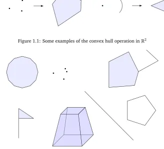
Figure 1.1: Some examples of the convex hull operation inR2

Figure 1.2: A medley of different polyhedra inR3. Each connected region is a polyhedron, as is the union of any number of those regions.

Polytopes and polyhedra. Every polyhedron considered here lives in some Euclidean spaceRn. Takex0, . . . ,xd∈Rn. Anaffine combinationofx0, . . . ,xdis a pointr0x0+· · ·+ rdxd, specified by somer0, . . . ,rd∈Rsuch thatr0+· · ·+rd=1. Aconvex combinationis an affine combination in which additionally eachri¾0. Given a setS⊆Rn, itsconvex hullConvSis the collection of convex combinations of its elements. See Figure 1.1 for a couple of examples of the convex hull operation inR2. A subspaceS⊆Rnisconvex if ConvS=S. Apolytopeis the convex hull of a finite set. ApolyhedroninRnis a set which can be expressed as the finite union of polytopes. To get an idea of the variety of subspaces which fall under the term ‘polyhedron’, see Figure 1.2. Note that every polyhedron is closed and bounded, hence compact.

Simplices. A set of pointsx₀, . . . ,xd isaffinely independentif whenever: r₀x₀+· · ·+rdxd=0 and r0+· · ·+rd=0

we must have that r₀, . . . ,rd=0. This is equivalent to saying that the vectors: x₁−x₀, . . . ,xd−x0

(20)

Figure 1.3: A quintessential 0-,1-,2- and 3-simplex

d. The idea is that ad-simplex is the simplest kind of polyhedron of dimensiond. See Figure 1.3 for representations of some simplices of dimensions 0 to 3 (of course, not all simplices are soregular). In fact, as we shall soon see, every polyhedron can be decomposed into these basic building blocks.

PROPOSITION1.25. Every simplex determines its vertex set: two simplices coincide if and only if they share the same vertex set.

Proof. See[Mau80, Proposition 2.3.3, p. 32].

Afaceofσis the convex hullτof some non-empty subset of{x₀, . . . ,x_d_}(note thatτis then a simplex too). Writeτ´σ, andτ≺σifτ6=σ.

Sincex₀, . . . ,xdare affinely independent, every pointx∈σcan be expressed uniquely as a convex combinationx=r₀x₀+· · ·+rdxd. Call the tuple(r0, . . . ,rd)thebarycentric coordinates of x inσ. Thebarycentre σ_b ofσis the special point whose barycentric coordinates are(_d₊1₁, . . . ,_d1₊₁). Therelative interiorofσis defined:

Relint_σ:₌{r₀x₀+· · ·+rdxd∈σ|r0, . . . ,rd>0}

The relative interior ofσis ‘σwithout its boundary’ in the following sense. Theaffine subspace spanned byσis the set of all affine combinations ofx₀, . . . ,xd. Then the relative interior ofσcoincides with the topological interior ofσinside this affine subspace. Note that Cl Relintσ=σ, the closure being taken in the ambient spaceRn.

Triangulations. Asimplicial complexinRnis a finite setΣof simplices satisfying the following conditions.

(a) Σis≺-downwards-closed: wheneverσ∈Σandτ≺σwe haveτ∈Σ. (b) Ifσ,τ∈Σ, thenσ∩τis either empty or a common face ofσandτ. ThesupportofΣis the set|Σ|:₌S

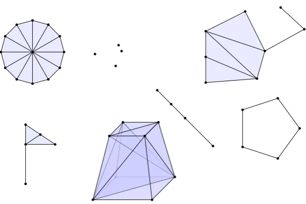
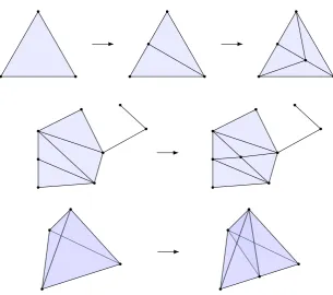
Σ. Note that by definition this set is automatically a polyhedron. We say that_Σis atriangulationof the polyhedron|Σ|. See Figure 1.4 for examples of triangulations of the polyhedra in Figure 1.2. Notice that_Σis a poset under

≺, called theface poset. Here we see the first suggestion of a connection with logic via Kripke frames. AsubcomplexofΣis subset which is itself a simplicial complex. Note that a subcomplex, as a poset, is precisely a downwards-closed set. Givenσ∈Σ, itsopen star is defined:

o(σ):₌[_{Relint(τ)|τ∈Σandσ⊆τ}

(21)

[image:21.595.144.452.110.315.2]

Figure 1.4: Triangulations of the medley of polyhedra given in Figure 1.2

In light of Proposition 1.26, for anyx∈ |Σ|let us writeσx_{for the unique}_σ

∈Σsuch thatx_∈Relintσ.

PROPOSITION1.27. LetΣbe a simplicial complex, takeτ∈Σandx_∈Relintτ. Then no proper faceσ≺τcontains x. This means thatσx _{is the inclusion-smallest simplex} containingx.

Proof. See[BMMP18, Lemma 3.1].

The next result is a basic fact of polyhedral geometry, and will play a fundamental role in connecting it with logic throughout this thesis. For_Σa triangulation andSa subspace of the ambient Euclidean spaceRn, define:

ΣS:={σ∈Σ|σ⊆S}

This, being a downwards-closed subset ofΣ, is a subcomplex ofΣ.

LEMMA 1.28(Triangulation Lemma). Any polyhedron admits a triangulation which simultaneously triangulates each of any fixed finite set of subpolyhedra. That is, for a collection of polyhedraP,Q₁, . . . ,Q_msuch that eachQ_i_⊆P, there is a triangulationΣof Psuch thatΣQi triangulatesQifor eachi.

Proof. See[RS72, Theorem 2.11 and Addendum 2.12, p. 16].

(22)

I should note however that the standard usage of ‘polyhedron’ is in fact more general than the present one. In PL topology, a ‘polyhedron’ is the union of alocally-finitesimplicial complex. The latter is defined as a (possibly infinite) setΣof simplices satisfying (a) and (b) in our definition of ‘simplicial complex’ above, subject to the condition that every point

x_∈S

Σhas an open neighbourhood which intersects only finitely-many simplices. Now, it is a standard fact that ‘compact polyhedra’ (in the more general sense) coincide with what we are referring to here as ‘polyhedra’ (see[RS72, Theorem 2.2, p. 12]). Hence we are effectively using the term ‘polyhedron’ as a shorthand for ‘compact polyhedron’; such usage is common in the literature (see, e.g. [Mau80]).

The dimension of a polyhedron. I said above that the dimension of ad-simplex

σ=x₀· · ·xdis exactlyd. Since the verticesx0, . . . ,xdare affinely independent, this is the same as the linear-space dimension of the affine subspace spanned by_σ. Thedimension of simplicial complex_Σis:

DimΣ:=max{Dimσ|σ∈Σ}

REMARK1.29. Note that DimΣ=height(Σ)as a poset.

PROPOSITION1.30. LetΣ,∆be simplicial complexes. If|Σ|=|∆|then DimΣ=Dim∆. Proof. See[Sta67, Proposition 1.6.12, p. 30].

With this in mind, we define thedimensionDimPof a polyhedronPto be the dimension of its triangulations. WhenP=∅, let DimP:₌−1.

Barycentric subdivision. Triangulations allow us in some ways to approximate the structure of a polyhedron. The finer the triangulation, the better the approximation. Barycentric subdivisions afford us a systematic way of generating finer and finer trian-gulations, starting from a base. This process allows us to extract, in the limit, all the relevant information about a polyhedron, in a way made precise by the Nerve Criterion, which we will meet in Chapter 2.

LetΣ,∆be simplicial complexes. ∆ is asubdivisionorrefinementofΣ, notation

∆ÃΣ, if|Σ|=|∆|and every simplex of∆is contained in a simplex ofΣ. LEMMA1.31. If∆ÃΣthen for everyσ∈Σwe have:

σ=[

{τ∈∆|τ⊆σ}

Proof. LetS:₌_{_τ_∈_∆_|_τ_⊆_σ_}. ClearlySS_⊆σ. Conversely, forx_∈σ, letτx

∈∆be such thatx_∈Relintτx_{. Since}_∆_refines_Σ_{, there is some}_ρ

∈Σsuch thatτx

⊆ρ; assume thatρis inclusion-minimal with this property. It follows from [Spa66, §3, Lemma 3, p. 121]that Relintτx⊆Relintρ, meaning thatx∈σ∩Relintρ. By condition (b) onΣ, we have thatσ∩ρis face ofρ. But then by Proposition 1.27,ρ´σ, since otherwise

σ∩ρwould be a proper face ofρcontainingx∈Relintρ. Thereforeτx⊆ρ⊆σso that x∈S

S.

(23)

[image:23.595.144.451.108.376.2]

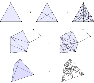
Figure 1.5: Examples of barycentric subdivision (the right-most tetrahedron is drawn without filled-in faces to aid clarity)

1.3 Logic and Polyhedra in Concert

Now that the background in logic and geometry has been established, we are in a position to connect the two. As indicated above, the initial contact is made between polyhedra and co-Heyting algebras. By exploiting duality, we then attain our connection with Heyting algebras and intuitionistic logic.

The co-Heyting algebra of sub-polyhedra. Fix throughout a polyhedron P. Let Sub_cPdenote the set of subpolyhedra ofP. We will see that Sub_cPis a co-Heyting algebra. PROPOSITION1.32. Sub_cPis a distributive lattice under∩and∪.

Proof. I follow[BMMP18, Corollary 2.12]; see also[Mau80, Proposition 2.3.6, p. 33]. First note that∅andPare minimal and maximal elements in SubcP. Also, by definition, the union of two polyhedra is again a polyhedron. So takeQ,R∈Sub_cPand consider Q_∩R. By the Triangulation Lemma 1.28, there is a triangulationΣofPsuch thatΣQ andΣRtriangulateQandRrespectively. SinceΣQandΣRare subcomplexes ofΣ, so is ΣQ∩ΣR. I will show that|ΣQ∩ΣR|=Q∩R, which will complete the proof. First, by definition|ΣQ∩ΣR| ⊆Q∩R. Conversely, take x∈Q∩R. Since|ΣQ|=Qand|ΣR|=R, there areσQ∈ΣQandσR∈ΣRsuch thatx ∈σQ∩σR. Then, by condition (b) in the definition of simplicial complex,σQ∩σRmust be a common face ofσQandσR. But then by condition (a), we must haveσQ∩σR∈ΣQ∩ΣR, so thatx∈ |ΣQ∩ΣR|.

(24)

Proof. I follow[BMMP18, Lemma 3.1]; see also[Mau80, Proposition 2.3.7, p. 34]. Take Q,Rsubpolyhedra ofP; I will show thatC:₌Cl(Q\R)is a polyhedron. First note that, by takingR∩Q, we may assume thatR⊆Q. Using the Triangulation Lemma 1.28, letΣ be a triangulation ofQsuch thatΣRtriangulatesR. Define:

∆:₌_{_σ_∈_Σ_{| ∃}_τ_∈_Σ_\_Σ_R:σ´τ}

Note that∆is a subtriangulation ofΣ. I will show that|∆|=C, which will give us the result. For the left-to-right inclusion, takeσ∈∆and letτ∈Σ\ΣRbe such thatσ´τ. Sinceτ=Cl Relintτ, it suffices to show that Relintτ⊆Q\R. So takex∈Relintτ, and note already that x∈Q. By Proposition 1.27,xis not contained in any proper face of

τ. Hence, by condition (b) on simplicial complexes, for anyρ∈Σ, ifx∈ρthenτ´ρ. Therefore, by choice ofτand condition (a) onΣR,x is not contained in any simplex of ΣR, whencex∈/R.

For the right-to-left inclusion, take x ∈ C. SinceC =Cl₍Q\R)in Rn, there is a sequence(xk)k∈N inQ\Rwhich converges to x. For each xk, the simplexσxk lies in Σ\ΣR. Since the latter is finite, there is a simplexτ∈Σ\ΣRwhich contains infinitely-manyxk’s. By restricting to thesexk’s, we obtain a subsequence(xki)i∈Nwhich lies inτ

and converges tox. But,τis closed, whencex∈τ⊆ |∆|.

Triangulation subalgebras and local-finiteness. Triangulations have an important algebraic correspondent, which will be used to show that Sub_cPis locally-finite. Take a triangulationΣofP. Its elements are themselves polyhedra, and in fact subpolyhedra ofP; thereforeΣ⊆ Sub_cP. Let P_c(Σ)be the sublattice ofC(P)generated byΣ. The following is Lemma 3.6 in[BMMP18].

PROPOSITION1.34. P_c₍_Σ₎is a co-Heyting subalgebra of Sub_cP.

Proof. Note that any non-emptyQ,R∈Pc(Σ)are by definition triangulated byΣQandΣR, respectively. But then it follows from the proof of Theorem 1.33 thatQ←R=Cl(Q\R) =

|∆|=S

∆, where:

∆:₌{σ∈Σ| ∃τ∈Σ\ΣR:σ´τ} ThereforeQ←R∈Pc(Σ).

Call a subalgebraA_⊆SubcPatriangulation subalgebraifA=Pc(Σ)for someΣ. The following two results are Lemma 3.2 and Corollary 3.7 in[BMMP18].

PROPOSITION1.35. Every finitely-generated subalgebra of Sub_cPis contained in some triangulation algebra.

Proof. TakeQ₁, . . . ,Qm∈SubcP. LetΣ, by the Triangulation Lemma 1.28, be a triangula-tion ofPwhich also triangulatesQ₁, . . . ,Qm. Note that the distributive latticeDgenerated byQ₁, . . . ,Qmis contained in Pc(Σ)by definition. Further, ifR,S∈DthenR←S∈Pc(Σ) just as in the proof of Proposition 1.34. Therefore the subalgebra generated byQ₁, . . . ,Qm is contained in P_c(Σ).

COROLLARY1.36. Sub_cPis locally-finite.

Proof. This follows from Proposition 1.35 since every triangulation subalgebra Pc(Σ)is finite.

(25)

PROPOSITION1.37. (1) Triangulation algebras determine their corresponding trian-gulations. That is, for any two triangulations Σand ∆, if P_c(Σ) =P_c(∆)then

Σ=∆.

(2) IfΣand∆are triangulations which are isomorphic as posets then P_c(Σ)∼₌P_c(∆). (3) If∆refinesΣ, then P_c(Σ)is a subalgebra of P_c(∆).

Proof. (1) It follows from conditions (a) and (b) on simplicial complexes that Pc(Σ) consists exactly of the unions of elements of Σ, and similarly for ∆. Assume Pc(Σ) =Pc(∆)and takeσ∈Σ. Thenσ∈Pc(∆), soσ=

S

Sfor someS⊆∆, and similarly eachτ∈Sisτ=ST_τfor someT_τ⊆Σ. Hence:

σ=[ [ τ∈S

T_τ

But then by condition (b) onΣ, everyρ∈S

τ∈STτ must either be equal toσor be a proper face ofσ. Since Relintσcontains no proper face ofσ, we must have

σ∈T_τfor someτ∈S. But thenσ⊆τ⊆σ, and soσ∈∆. Applying this argument also in the other direction, we get thatΣ=∆.

(2) This is immediate from the definition of Pc.

(3) By Lemma 1.31, everyσ∈Σis the union of simplices in∆. WhenceΣ⊆P_c(∆). Therefore, by definition Pc(Σ)⊆Pc(∆).

The other side of the coin: the Heyting algebra SuboP. Now that we have es-tablished the locally-finite co-Heyting algebra Sub_cP, it is time to recast it as a Heyting algebra. To obtain a concrete representation, let us take inspiration from the topological case above, and apply the complement operator−C_{. Following} _[_BMMP18_]_{, an} _open

subpolyhedronofPis the set-theoretic complement of a (closed) subpolyhedron inP. Let Sub_oPbe the set of open subpolyhedra inP. By the duals of Proposition 1.32, Theo-rem 1.33, and Corollary 1.36, this is a locally-finite Heyting algebra, and a subalgebra ofO(P). Given any triangulationΣofP, let P_o(Σ)be the Heyting subalgebra generated by the complements of the simplices inΣ— i.e. the dual to the co-Heyting subalgebra Pc(Σ).

Note that ‘open subpolyhedra’ are not ‘polyhedra’ in the sense used here. They are however ‘polyhedra’ in the more general sense of PL topology. Indeed, one might think to use this more general notion as an alternative way of constructing an algebra of open polyhedra. But in fact, the open PL-polyhedra aretoogeneral for our purposes: the open PL-polyhedra inRnare exactly the arbitrary open sets ofRn(see[FP90, Corollary 3.2.22, p. 109]). Thus, the consideration here of open subpolyhedra, though not standard, paves the way to a new semantics for intuitionistic logic by reinstating the duality between open and closed sets.

DEFINITION1.38(Polyhedral completeness). A logicL ispolyhedrally-completeif it is the logic of a class of polyhedra.

(26)

And the modal case. By Theorem 1.22, there is anS4-algebraM such thatM= Sub_oP. In fact, there is such an algebra with a rather natural form, as considered in [Gab+18]. Anopen half-spaceinRnis the set of points(x1, . . . ,xn)satisfying, for some a₁, . . . ,a_n,b_∈_R:

a₁x₁+_{· · ·}+a_nx_n<b

The correspondingclosed half-spaceis the set of points satisfying: a₁x₁+_{· · ·}+a_nx_n_¶b

Define apolytopal setinRnto be a subspace which is the intersection of finitely-many open and closed half-spaces. More compactly, we can say that a polytopal set is the solution set of a system of linear inequalities. Apolyhedral setis then the union of finitely-many polytopal sets.

Given any polyhedral setP, let SubPdenote the collection of polyhedral subsets. This is a modal algebra whenis interpreted as the topological interior operator. Moreover, we have the following.

PROPOSITION1.40. SubPis a Grzegorczyk algebra. Proof. This follows from[Fon18, Theorem 3.8.3, p. 105].

PROPOSITION1.41. WhenPis a polyhedron (in our sense), we have₍SubP₎₌Sub_oP. Proof. See[Fon18, Theorem 3.5.1, p. 86].

Using this modal algebra, one can proceed to investigate the modal logic of polyhedra. However, the Blok-Esakia Theorem tells us that this investigation is essentially the same as that of the intuitionistic logic of polyhedra. Indeed, the isomorphismσallows us to move freely between the resulting logics. Since it is thus redundant to keep track of both kinds of logic, from now on I will focus solely on the intuitionistic side.

Posets dual to triangulation subalgebras. Fix a triangulationΣofP. We investigate the triangulation subalgebra Po(Σ)a little more. First, recall the definition (page 19) of the open star o(σ)of a simplexσ∈Σ.

PROPOSITION 1.42. The open star of a simplex is an open subpolyhedron. That is, o(σ)∈P_o(Σ).

Proof. See[Mau80, Proposition 2.4.3, p. 43]and[BMMP18, p. 12]. Define:

γ↑_{: Up}_Σ_→_P

o(Σ) U7→[

σ∈U

Relintσ

To see thatU∈UpΣreally lands in Po(Σ), note that:

γ↑₍_U_{) =} [ σ∈U

γ↑₍_↑₍_σ₎₎

= [

σ∈U

[

{Relint(τ)|τ∈Σandσ⊆τ}

= [

(27)

(a)

x₀

x₁

x₃

x₄

x₂

(b) (c)

x₀ x₁ x₂ x₃ x₄

Figure 1.6: Computation of the face poset: (a) a 2-dimensional polyhedron, (b) a triangulation of this polyhedron, and (c) the face poset of this triangulation.

SinceUis finite, by Proposition 1.42 we get thatγ↑(U)∈Po(Σ).

PROPOSITION1.43. γ↑gives an isomorphism of Heyting algebras UpΣ∼₌P_o(Σ). Proof. See[BMMP18, Lemma 4.3].

This proposition gives a concrete description of P_o(Σ)and means thatΣ, as a face poset, is its dual. The characterisation is very handy, since the simplicial complexΣtends to be much easier to visualise than the algebra P_o(Σ). See Figure 1.6 for an example of the computation of this poset. For any polyhedronP, we have the following chain of equalities.

Logic(P) =Logic(SuboP)

=Logic₍B|Bfinitely-generated subalgebra of Sub_oP) (Proposition 1.10)

=Logic(Po(Σ)|Σtriangulation ofP) (Proposition 1.35)

=Logic(UpΣ|Σtriangulation ofP) (Proposition 1.43)

=Logic(Σ|Σtriangulation ofP) (Proposition 1.14) This leads us to our first maxim.

MAXIMI. The logic of a polyhedron is the logic of its triangulations.

Thus we obtain a purely combinatorial description of Logic(P)in terms finite objects: its triangulations.

Using the isomorphism in Proposition 1.43, we can also define thedimensionof an open polyhedronQ∈Po(Σ)to be Dim(Q):=height(↓(U)), whereU= (γ↑)−1(Q). PROPOSITION1.44. ClQis a polyhedron and Dim(Q) =Dim(ClQ). Hence the dimension ofQis independent of the triangulationΣ.

Proof. We have, by Proposition 1.43, that: Q=γ↑(U) = [

σ∈U

Relintσ

Hence, asUis finite:

ClQ= [

σ∈U

Cl Relintσ= [

σ∈U

(28)

noting that, since↓Uis closed it is a subcomplex ofΣ. But now: Dim(|↓U|) =height(↓U) =Dim(Q)

Polyhedral maps. Here I will present some basic interactions between logic and polyhedra at the level of morphisms. These results come from joint work with Nick Bezhanishvili, David Gabelaia and Vincenzo Marra. LetPbe a polyhedron andF be a poset. A functionf:P_→F is apolyhedral mapif the preimage of any open set inF is an open subpolyhedron ofP. Note that such a function is continuous.

PROPOSITION1.45. Let f:P→F be a function from a polyhedronPto a finite posetF, and write f∗:₌ f−1[−]:P(F)→ P(P)for the inverse image function.

(1) The function f is polyhedral if and only iff∗descends to a lattice homomorphism f∗: UpF →Sub_oP.

(2) The functionf is polyhedral and open if and only iff∗descends to a homomorphism of Heyting algebras f∗: UpF→Sub_oP.

Proof. Clearly f∗is a homomorphism of Boolean algebras, so (1) follows from the defini-tions. As for (2), let us first assume that f is polyhedral and open, and takeU,V _∈UpF with the aim of showing that f∗(U_→V) =f∗(U)_→f∗(V). The left-to-right inclusion follows from the fact that f∗is a lattice homomorphism. For the right-to-left, writingXC for the complement ofX, we have the following chain of inclusions.

f[f∗(U)→f∗(V)] =f Int f−1[U]C∪f−1[V]

⊆Int ff−1[U]C∪f−1[V] (f is open)

=Int ff−1[UC_∪V]

⊆Int(UC_∪V)

=U→V

Applyingf∗=f−1to both sides, we get thatf∗(U)→f∗(V)⊆ f∗(U→V).

For the converse implication, assume that f∗is a Heyting algebra homomorphism. By (1), f is polyhedral, so takeW ⊆ F with the aim of showing that f−1[IntW] = Int₍f−1[W]). First let A :₌ Int₍₍↑W)C∪W)∪Int₍WC) and B :₌ IntW. A routine calculation verifies thatAC∪B=W, and moreover thatA,B∈UpF. Then:

f−1[IntW] =f∗[A→B]

=f∗[A]→f∗[B] (f∗is a homomorphism)

=Int(f∗[A]C∪f∗[B])

=Int(f∗[AC∪B])

=Int(f−1[W])

LetΣbe a simplicial complex andF be a poset. Given any function f:Σ→F, define the map bf:|Σ| →F by:

b

f(x):₌f(σx)

(29)

Proof. For anyU∈UpF, we have that: b

f−1[U] =[{Relintσ|σ∈Σandσ∈f−1[U]}=γ↑(f−1[U])

Since f is monotonic, f−1[U]is upwards-closed in_Σ, whence as above fb−1[U]is an open sub-polyhedron of|Σ|. Now take an open setW⊆ |Σ|, with the aim of showing that

b

f[W]is open. Define:

Σ#W:₌_{_σ_∈_Σ_|Relint(σ)∩W6=∅} Then:

b

f[W] =_{f(σx)_|x_∈W_}=f[Σ#W]

Ifσ∈Σ#W andσ´τ, then asσ⊆τ=Cl RelintτandW is open, we haveτ∈Σ#W; i.e.Σ#Wis upwards-closed. But now, f is open and so bf[W]is also upwards-closed.

Another important class of maps is that of PL homeomorphisms. First, for anyX,Y⊆

Rn, a functionX →Y is anaffine mapif it is of the formx7→M x+b, whereMis a linear transformation andb∈Rn. Now letP,Qbe polyhedra. A homeomorphism f:P→Qis piecewise-linearif there is a triangulationΣofPsuch that for eachσ∈Σthe restriction

f|σ is affine. Call such mapsPL homeomorphismsfor short.

PROPOSITION1.47. The inverse of a PL homeomorphism is a PL homeomorphism. Proof. See[RS72, p. 6].

PROPOSITION 1.48. Any PL homeomorphism f:P →Q between polyhedra, along with its inverse g:Q_→P, induce mutually inverse isomorphisms of Heyting algebras

f∗: SuboQ→SuboPandg∗: SuboP→SuboQ.

(30)

Chapter 2

Nerves and Triangulations

In this chapter, I introduce the notion of the nerve of a poset. This is a classical construction originally due to Pavel Alexandrov[Ale98], which has found numerous applications in geometry, topology and combinatorics (see e.g.[Bjö95]). The nerve has an important place in the present thesis, and it will be used to deepen the logic-geometry connection established in Chapter 1.

2.1 Nerves for Geometric Realisation

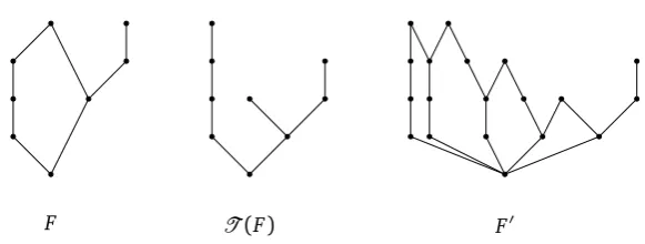
DEFINITION2.1(Nerve of a poset). Thenerve_N(F)of a posetF is the collection of non-empty finite chains inF ordered by inclusion.

See Figure 2.1 for an example of the nerve construction, and compare to Figure 1.6. A key fact about the nerve and its relation to logic is that there is always a p-morphism

N(F)→F.

DEFINITION2.2. Let max:N(F)→Fbe the map which sends a chainX to its maximal element.

PROPOSITION2.3. max:N(F)→F is a p-morphism.

x₂ x₁

x₀ x₃

x₄

F

{x₀} {x₁} {x₂} {x₃} {x₄} N(F)