Preferred, small scale foraging areas of two Southern Ocean fur seal species are not determined by habitat characteristics

RESEARCH ARTICLE

Preferred, small-scale foraging areas

of two Southern Ocean fur seal species are

not determined by habitat characteristics

Mia Wege

_{, P. J. Nico de Bruyn}

_{, Mark A. Hindell}

_{, Mary‑Anne Lea}

_{and Marthán N. Bester}

Abstract

Background: To understand and predict the distribution of foragers, it is crucial to identify the factors that affect individual movement decisions at different scales. Individuals are expected to adjust their foraging movements to the hierarchical spatial distribution of resources. At a small local scale, spatial segregation in foraging habitat happens among individuals of closely situated colonies. If foraging segregation is due to differences in distribution of resources, we would expect segregated foraging areas to have divergent habitat characteristics.

Results: We investigated how environmental characteristics of preferred foraging areas differ between two closely situated Subantarctic fur seal (Arctocephalus tropicalis) colonies and a single Antarctic fur seal (A. gazella) colony that forage in different pelagic areas even though they are located well within each other’s foraging range. We further investigated the influence of the seasonal cycle on those environmental factors. This study used tracking data from 121 adult female Subantarctic and Antarctic fur seals, collected during summer and winter (2009–2015), from three different colonies. Boosted Regression Tree species distribution models were used to determine key environmental variables associated with areas of fur seal restricted search behaviour. There were no differences in the relative influ‑ ence of key environmental variables between colonies and seasons. The variables with the most influence for each colony and season were latitude, longitude and magnitude of sea‑currents. The influence of latitude and longitude is a by‑product of the species’ distinct foraging areas, despite the close proximity (< 25 km) of the colonies. The pre‑ dicted potential foraging areas for each colony changed from summer to winter, reflecting the seasonal cycle of the Southern Ocean. The model predicted that the potential foraging areas of females from the three colonies should overlap, and the fact they do not in reality indicates that factors other than environmental are influencing the location of each colony’s foraging area.

Conclusions: The results indicated that small scale spatial segregation of foraging habitats is not driven by bottom‑ up processes. It is therefore important to also consider other potential drivers, e.g. competition, information transfer, and memory, to understand animal foraging decisions and movements.

Keywords: Arctocephalus, Boosted regression tree, Foraging behaviour, Foraging segregation, Machine learning, Marion Island, Niche, Sympatry

© The Author(s) 2019. This article is distributed under the terms of the Creative Commons Attribution 4.0 International License (http://creat iveco mmons .org/licen ses/by/4.0/), which permits unrestricted use, distribution, and reproduction in any medium, provided you give appropriate credit to the original author(s) and the source, provide a link to the Creative Commons license, and indicate if changes were made. The Creative Commons Public Domain Dedication waiver (http://creativecommons.org/ publicdomain/zero/1.0/) applies to the data made available in this article, unless otherwise stated.

Open Access

*Correspondence: mia.wege@gmail.com

1 _{Mammal Research Institute, Department of Zoology & Entomology,}

Background

The presence and abundance of prey play a crucial role in the distribution of marine predators living in highly seasonal environments. However, marine ecosystems

are dynamic and complex [1] with resources constantly

moving in three-dimensional space. Scale-dependent physical and biological processes determine the

distribu-tion of nutrients and subsequent productivity [2],

abun-dance of grazers, prey, and consequently, predators [3–5].

Bathymetry, sea-surface temperature, frontal regions, meso-scale eddies, wind and currents are examples of environmental variables that influence marine

preda-tors [6–10]. Marine predators, high profile components

of marine ecosystems, feed at a range of trophic levels within a variety of marine habitats, and are sensitive to

shifts in the aforementioned bottom-up processes [11].

Alterations to the productivity, abundance, and distri-bution of lower trophic level organisms therefore affect many aspects of top-predator life history and ultimately

influence their population growth [12, 13]. This leads to

the common assumption that facets of their behaviour, health, reproductive output, and subsequent population growth status are indicative of the productivity and

qual-ity of food within the ocean [13, 14]. As a result, marine

predators are thought to be ideal sentinels to monitor

changes in marine ecosystems [13].

Despite the major influence of external, environmental bottom-up processes on foraging behaviour of predators, these are not the only determinants of predator foraging behaviour. Other drivers, such as age (experience), sex, species interactions, and breeding status that are a few aspects of demography that contribute to variations in foraging behaviour and subsequent population

dynam-ics [15–21]. However, the dictators of some foraging

behaviours are still unknown or currently only theoreti-cal. Spatial segregation between conspecifics from neigh-bouring colonies is one such example. Initially, spatial segregation between individuals from distant colonies were thought to occur because of differential

bottom-up processes that drive foraging preferences [22, 23]. For

spatially restricted species, such as central-place forag-ers, the distance required to travel from the colony to the foraging areas of distant colonies would be energetically too expensive and therefore force individuals to forage

closer to their own colonies [24, 25]. However, recent

research indicate that even closely situated colonies that are well within each other’s foraging range also segregate spatially. Such segregation occurs in, for example, Adélie

penguins (Pygoscelis adeliae) [26, 27], Northern fur

seals (Callorhinus ursinus) [28, 29], Macaroni penguins

(Eudyptes chrysolophus) [30], and Magellanic penguins

(Spheniscus magellanicus) [31]. Current hypotheses

sug-gest that this small-scale spatial segregation is driven by

competitive exclusion, which is then further enhanced by private information (i.e. memory) and public informa-tion, where the colony acts as an information centre and individuals inadvertently transfer knowledge to conspe-cifics either at the colony when they are observed depart-ing to or returndepart-ing from a direction (i.e. the information

centre hypothesis [32]. However, to date it has not been

tested how common environmental bottom-up drivers of these closely situated colonies that forage in disparate regions, differ from each other.

Sympatric female Subantarctic fur seals (Arctocepha-lus tropicalis; SAFS) and Antarctic fur seals (A. gazella; AFS) at sub-Antarctic Marion Island have species- and colony-specific foraging areas. They also change these

foraging areas from summer to winter [33], maintain

minimal overlap with foragers from neighbouring colo-nies, despite the colonies being situated well within the travelling range of both species. We aim to understand how environmental characteristics of preferred forag-ing areas differ between two SAFS colonies and an AFS colony, at Marion Island; and how the seasonal cycle of the Southern Ocean modulates these characteristics. We quantify the at-sea distribution and foraging habitats of female SAFS and AFS from three closely situated colo-nies across summer and winter. We hypothesize that the environmental variables associated with each of the three colonies’ foraging locations will not differ and that model predicted potential foraging areas among the three colo-nies overlap. However, due to the commanding role the seasonal cycle in the Southern Ocean plays on primary productivity, and prey distribution and abundance, we expect environmental variables associated with forag-ing locations for each colony to change from summer to winter. We ask three key questions: (1) does the pre-ferred foraging areas of female fur seals from the three study colonies differ in environmental indicators? (2) Do these environmental indicators change from summer to winter? (3) Are the environmental indicators of preferred foraging areas present in areas associated with foraging of the neighbouring colonies?

Results

At-sea locations for 121 lactating females are presented from 44 AFS  from a high-density colony (summer: 24, winter: 20; hereafter HD_AFS); 40 SAFS females  from the high-density colony (summer: 19, winter: 21; hereaf-ter HD_SAFS) and 37 SAFS females  from the low-den-sity colony (summer: 15, winter: 22; hereafter LD_SAFS) between 2009 and 2015. The data comprise 617 foraging trips (range: 1–16 trips per female) of which 560 (91%)

were complete and 36 (9%) incomplete (Additional file 1:

estimates were classified as restricted search areas and, 54,367 (58.18%) as transit: only 67 (< 1%) locations could not be classified and were subsequently removed from further analyses.

Determining coverage of true colony foraging areas

Summer individuals from all three colonies reached an asymptote of the number of new grid cells added within < 10 individuals whereas winter individuals never

fully reached an asymptote (Additional file 1: Fig. S2).

Winter females’ inflexion point of the number of new

0.25° × 0.25° cells added was between 20 and 25 grid cells,

with HD_AFS showing the least decrease in number of cells added with each new tracked female added

(Addi-tional file 1: Fig. S2).

Species distribution models

The best learning rate, tree complexity, and bagging frac-tion that resulted in the least amount of residual deviance

were learning rate = 0.0005, tree complexity = 5, and

bag-ging fraction = 0.5, respectively (Table 1).

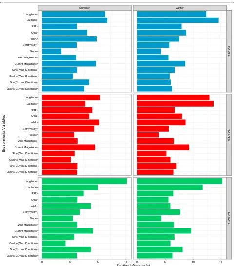
All six final BRT models include all but one (mean sea-sonal frontal region) of the co-variates. The relative influ-ence of each of the variables differed very little among the

models (Fig. 1). Longitude and latitude were among the

top three ranked environmental variables for all models,

except the HD_SAFS summer model (Fig. 1). Aside from

latitude and longitude, ocean current magnitude was the only variable which was within the top five variables of all BRT models. The other five top environmental variables, all contributing the most to relative influence of the final BRT models, were SST, bathymetry, Chla, and sshA and the sine of ocean current direction (i.e. the ‘eastness’ of the current).

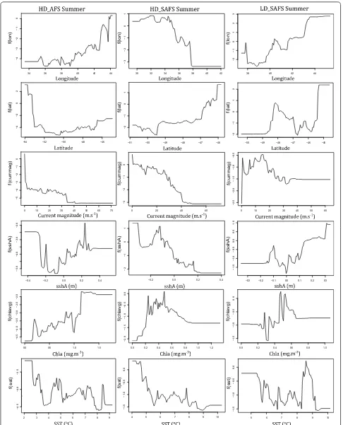
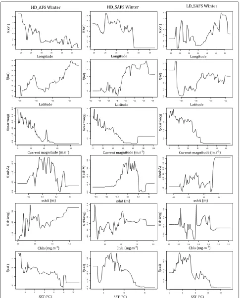
Although the relative contribution of the environmen-tal predictor variables did not differ greatly between colonies and seasons, the response curves (relationships) between the probability of restricted search and the pre-dictor variables differed among colonies and seasons. The response curves for most of the behavioural activity

predictors for the seals were non-linear (Figs. 2, 3;

Addi-tional file 1: Figs. S3–S8). The relationship between the

probability of restricted search and the predictor varia-bles differed between colonies with the biggest difference in the response curves of latitude and longitude between colonies. The relationship between restricted search areas and current magnitude was negative across all

sea-sons and colonies (Figs. 2, 3). Between seasons the

big-gest differences were the values of the predictor variables where the peaks and troughs of restricted search

prob-ability occurred (Figs. 2, 3; Additional file 1: Figs. S3–S8).

Predicted potential area of restricted search regions

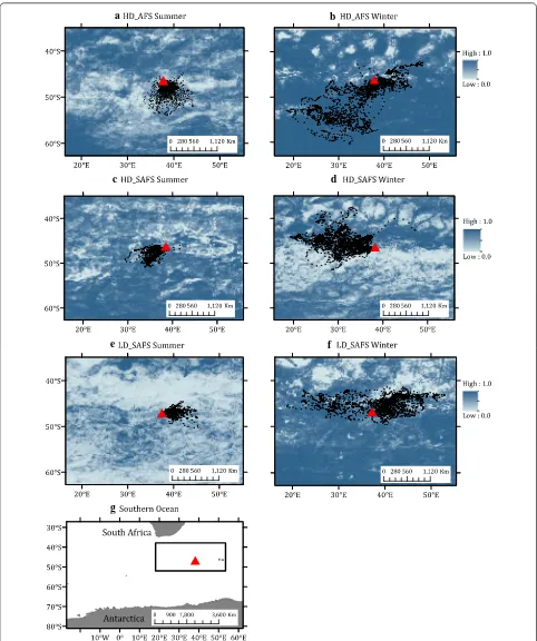
During summer months, potential restricted search regions were predicted to be available within the areas utilized by seals from each colony as well as the other two

colonies’ foraging domains (Fig. 4a, c, e). HD_AFS and

LD_SAFS females mostly only have potential available restricted search regions to the south of Marion Island

(Fig. 4a, e), whereas HD_SAFS had options available to

areas off the north-west of the island too (Fig. 4c). Some

HD_SAFS females spent time in a non-predicted region

due-west of Marion Island (Fig. 4c). During winter, HD_

AFS females had regions available all-around Marion Island except for some patches north and north-west

of the island (Fig. 4b). HD_SAFS females had potential

restricted search areas available to the west, north-west,

and east of Marion Island (Fig. 4d), whereas LD_SAFS

females had areas all around Marion Island available,

except for a region north-east of the island (Fig. 4f).

Discussion

Predators are sensitive to bottom-up processes, however, here, we demonstrated that there are no pronounced differences in environmental variables associated with distinct, neighbouring foraging areas of lactating SAFS and AFS. Furthermore, the relative contribution of these variables associated with restricted search changed little from summer to winter. Model predicted potential forag-ing areas did change from summer to winter, indicatforag-ing

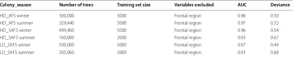
Table 1 Final parameters used for each of the boosted regression tree models

HD_SAFS high-density Subantarctic fur seal colony, LD_SAFS the low-density Subantarctic fur seal colony, HD_AFS the high-density Antarctic fur seal colony, AUC the area under curve of the receiver operating characteristic

Colony_season Number of trees Training set size Variables excluded AUC Deviance

that seasonal fluctuations and spatial movements of prey aggregations and its availability are likely driving seasonal changes in fur seal movements. The models predicted

that the potential foraging areas of females from the three colonies should overlap, and that these did not, indicates that factors other than environmental characteristics

Summer Winter

HD_AFS

HD_SAF

S

LD_SAF

S

0 5 10 15 0 5 10 15

Cosine(Current Direction) Sine(Current Direction) Cosine(Wind Direction) Sine(Wind Direction) Current Magnitude Wind Magnitude Slope Bathymetry sshA Chla SST Latitude Longitude

Cosine(Current Direction) Sine(Current Direction) Cosine(Wind Direction) Sine(Wind Direction) Current Magnitude Wind Magnitude Slope Bathymetry sshA Chla SST Latitude Longitude

Cosine(Current Direction) Sine(Current Direction) Cosine(Wind Direction) Sine(Wind Direction) Current Magnitude Wind Magnitude Slope Bathymetry sshA Chla SST Latitude Longitude

Relative Influence (%)

En

vironmental

Va

riab

les

0 20 40 60 −3 −2 −10 f(curr mag)

0 10 20 30 40 50 60

−2. 5− 2. 0 −1.5 −1.0 −0. 5 f(curr mag)

−54 −52 −50 −48 −46

−4

−2

02

f(lat)

0.0 0.2 0.4 0.6 0.8 1.0 1.2

−2.0 −1.5 −1.0 −0.5 0.0 f(chla vg )

−0.2 0.0 0.2 0.4

− 2 −1 01 f(sshA )

30 32 34 36 38 40 42

−3 − 2 − 10 1 f(lon)

−51 −50 −49 −48 −47 −46

−2

−1

01

f(lat

)

4 5 6 7 8 9 10

−1.5 −1.0 −0.5 0. 0 f(sst )

0 10 20 30 40 50 60 70

−5 −4 −3− 2 −1 0 f(curr mag)

2 3 4 5 6 7 8 9

−4.5

−4.0

−3.5

f(sst

)

34 36 38 40 42 44

− 4− 3 −2 −1 0 f(lon)

0.0 0.5 1.0 1.5

−4.5 −4.0 −3.5 −3.0 −2.5 −2.0 f(chla vg )

−0.4 −0.2 0.0 0.2 0.4

− 5. 0− 4. 0− 3. 0− 2. 0 f(sshA)

38 40 42 44

−2

−1

012

3

f(lon)

−50 −49 −48 −47 −46 −45

−

2−

10

12

f(lat)

5 6 7 8 9 10

−1.5 −1.0 −0. 50 .0 f(sst)

−0.3 −0.2 −0.1 0.0 0.1 0.2 0.3

−1. 5 −1.0 −0.5 0. 00 .5 1. 0 f(sshA)

0.0 0.2 0.4 0.6 0.8 1.0

−1.5 −1.0 −0.5 0. 0 f(chla vg )

0 2 4 6 8 10 −2 −1 01 f(sst )

−0.2 0.0 0.2 0.4

−2.0 −1.5 − 1. 0− 0. 5 f(sshA)

0 20 40 60 80

−2.0 −1.5 −1.0 −0.5 0. 00 .5 f(curr mag)

20 25 30 35 40 45

−2

−1

0123

f(lon)

0.0 0.5 1.0 1.5

−1.0 −0.5 0. 0 f(chla vg)

−60 −55 −50 −45

− 4− 3− 2 −1 012 3 f(lat)

0 20 40 60 80 100 120

−2 −1 01 2 f(curr mag)

−0.6 −0.4 −0.2 0.0 0.2 0.4

−1.5 −1.0 −0.5 0. 00 .5 f(sshA)

−52 −50 −48 −46 −44 −42 −40 −38

−1

012

3

f(lat)

20 25 30 35 40 45

−4 −3 − 2− 10 12 f(lon)

0.5 1.0 1.5 2.0

−0. 50 .0 0. 51 .0 1. 52 .0 f(chla vg)

5 10 15

−1.5 −1.0 −0.5 0. 00 .5 f(sst )

0.0 0.2 0.4 0.6 0.8 1.0 1.2

−1.0 −0.5 0. 00 .5 f(chla vg )

4 6 8 10 12

−1.5 −1.0 − 0. 5 f(sst)

−48 −46 −44 −42

−3 −2 −1 01 2 f(lat)

−0.2 0.0 0.2 0.4

− 1. 5 −0.5 0. 00 .5 1. 01 .5 f(sshA)

0 10 20 30 40 50 60

−3

−2−

10

f(curr

mag)

20 25 30 35 40 45 50

−3

−2

−1

0123

f(lon)

a b

c d

e f

g

influence the location of female foraging areas for each colony.

Females from all colonies and seasons displayed less restricted search in areas with stronger ocean current. Faster current speed precludes the formation of closed-circulation cells and the subsequent retention of water bodies leading to upwelling and enhanced primary

pro-duction [34]. Marion Island lies in a region of enhanced

eddy kinetic energy caused by the eastward flowing Ant-arctic Circumpolar Current’s collision with the

South-west Indian Ridge upstream of the island [35–37]. During

summer, females from the HD_AFS and LD_SAFS col-onies had higher probability of restricted search in areas with positive sshA, whereas HD_SAFS had more

restricted search in negative sshA (Fig. 2). During winter,

females from all three colonies foraged more in regions of positive sshA. Positive sshA are indicative of cold-core cyclonic eddies that spin up to the surface. Cyclonic eddies have higher concentrations of chla around the

edges of the eddies [36] and during winter could provide

pockets of productivity within an otherwise resource depleted habitat. In this area of the Southern Ocean,

juvenile southern elephant seals (Mirounga leonina) [38]

were also shown to avoid “intense eddy features” and sim-ilarly in the summer foraged in areas with positive sshA values. In the winter however, juvenile elephant seals for-aged at the edges of eddies, where sshA slope values are

high [38]. Similarly, grey-headed albatross (Thalassarche

chrysostoma) also foraged in sshA; during chick-rearing period in particular around the edges of these anomalies

formed in the South-west Indian Ridge [39].

Although sea-surface temperature contributed little to

relative influence on all six models (Figs. 2, 3) there are

clear peaks and troughs in the response curves at 4  °C and 8 °C. These are the surface isotherms where the Polar Front and the sub-Antarctic Front are typically found

[35]. Seasonal mean frontal region was the only variable

dropped from the BRT models, which suggested little or no contribution to restricted search behaviour. However, diving behaviour of both fur seal species at Marion Island

are influenced by frontal regions [40]. Foraging behaviour

of SAFS females from neighbouring Prince Edward Island

(46°37′47″S; 37°56′17″E) and distant Amsterdam Island

(37°49′33″S; 77°33′17″E) are also influenced by frontal

regions, specifically the sub-Antarctic Front [41–43]. It

is therefore possible that averaging frontal regions across multiple years (this study) did not capture the scale at which frontal regions influence SAFS and AFS foraging behaviour at Marion Island.

Wind strength and direction contributed very little to all models. This observation contrasts recent findings of winter tracking of females from a low-density AFS (LD_

AFS) colony, also on Marion Island [44]. Arthur et al. [45]

used time-spent in an area to match the error uncertainty associated with geo-location sensing tags. It is unlikely

that the dissimilarities between this study and [44] is due

to differences between species, seasons or colonies given that this study found little differences among the three other colonies at the same island location. Furthermore, winter foraging areas between the HD_AFS colony and

the LD_AFS colony overlapped greatly [18, 44, 55]. Given

that environmental correlates influence predator foraging behaviour differently across a hierarchy of spatial scales

[46], this difference might be due to larger scale areas

used by [44] to infer restricted search areas.

Ultimately, the differences in relative influence of key environmental variables between colonies or seasons were small and nuanced. Latitude and longitude, the two most important variables in the final model, were also the two variables of which the response curves differed the most among colonies. Although predictions using interpola-tions of habitat models are useful to expand on the poten-tial habitats of marine species for conservation practices

[11, 25, 44], it should also be taken into account that these

are not always “realistic” foraging areas for species spatio-temporally restricted in their movements away from their colonies. In this study, habitat predicted available foraging areas overlapped among colonies and seasons. We suggest that the aforementioned, and the dominating influence of latitude and longitude, is potentially a by-product of the intrinsically-driven colony-preferred foraging directions

of the fur seal females [55]. At a small local scale (i.e., at

the same island), commonly measured environmental variables, as a proxy for some bottom-up processes, are not the drivers of spatial segregation of core habitat uti-lisation areas between colonies; otherwise seals would have foraged in a neighbouring colony’s core foraging areas due to the negligible swimming distances between them. Environmental correlates certainly do influence predator foraging behaviour at a larger regional scale and when comparing environmental drivers of predator forag-ing behaviour between distantly located islands it would mostly differ due to the local environment experienced by

the predators at each of the separate island colonies [24,

47, 48]. This only gives one an indication of the dominant

environmental drivers of prey-aggregations within the regional scale surrounding that colony. For example, dur-ing winter the preferred travelldur-ing directions of kdur-ing pen-guins (Aptenodytes patagonicus) from the Falkland Islands are dominated by the local, northward-flowing Falkland

Current [49]; or the influence of the shelf-break of the

Kerguelen Plateau on the diving behaviour of Antarctic

fur seals [10]. Pinaud and Weimerskirch [37] showed how

types (intra-species). This was a broad-scale comparison between three distant islands (Amsterdam, Crozet and Kerguelen) and concluded that we need to study move-ments at smaller scales in relation to resource distribu-tion to understand scale-dependent foraging distribudistribu-tion of predators. Here, at a small local scale—the core forag-ing areas of fur seal females from three colonies that for-age in separate areas, but still experience the same local conditions (present study), are not only driven by prey

aggregations [50]. Several studies have found that

indi-viduals from neighbouring colonies of central-place forag-ers segregate from each other despite being situated well

within each other foraging range [28, 29, 51–53]. Often

the density or size of the colony has an influence on the home range size of a colony, i.e. offspring from smaller colonies are lighter presumably because parents had to

make longer foraging trips further afield [26, 51]. This is

explained through intra-specific competition, where the

larger colony outcompetes the smaller colony [19, 51].

However, density-dependent competition does not always drive spatial segregation between neighbouring colonies,

including here for fur seals at Marion Island [[55],52].

Current hypotheses suggest that information transfer, memory, and learned behaviours could drive this spatial

segregation [28, 32, 51, 52, 54], although the actual

mech-anisms behind this remain largely unstudied [28].

The model predicted potential foraging areas shifted from summer to winter for all study colonies on Marion Island (this study), akin to SAFS from Prince Edward Island, where predicted foraging regions also changed seasonally to areas further afield from the study colony

in winter [41]. As environmental conditions change with

the seasons (e.g. water temperatures decreasing, shift-ing wind patterns and current changes), this would most likely cause the locations of prey aggregations to shift

from summer to winter [56, 57] and subsequently result

in the shift of potential foraging habitat.

Predicted potential foraging areas of HD_AFS females span almost the entire region surrounding Marion Island. This result should be interpreted with caution given that the cumulative information analysis suggested that the available tracking data for HD_AFS winter females did not adequately capture the spatial use patterns of the entire colony. Therefore, we have little confidence in the HD_AFS winter predicted foraging areas and more track-ing data are needed to accurately predict alternative for-aging areas around Marion Island.

Conclusions

The results indicated that there are no pronounced dif-ferences in environmental variables associated with dis-tinct, neighbouring foraging areas of lactating SAFS and AFS. Furthermore, the relative contribution of these

variables associated with restricted search changed little from summer to winter. Model predicted potential forag-ing areas did change from summer to winter, implicatforag-ing the seasonal fluctuations and spatial movements of prey aggregations and its availability. The models predicted that the potential foraging areas of females from the three colonies should overlap, and that these did not, indicates that small scale spatial segregation of foraging habitats is not driven by bottom-up processes. It is therefore impor-tant to also consider other potential drivers, e.g. compe-tition, information transfer, and memory, to understand animal foraging decisions and movements.

Methods

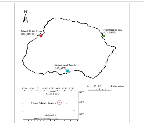
The three breeding colonies are situated around the coastline of sub-Antarctic Marion Island. Watertun-nel Beach, the high-density AFS colony, is situated on

the south coast (46°58′6.4″S; 37°44′39.73″E, hereafter

HD_AFS); Mixed Pickle Cove, the high-density SAFS

colony, is situated on the west coast (46°52′15.88″S;

37°38′18.27″E, hereafter HD_SAFS) and Rockhopper Bay,

the low-density SAFS colony is situated on the northeast

coast of Marion Island (46°52′13.33″S; 37°51′25.34″E,

hereafter LD_SAFS; Fig. 5). Fur seal densities at colonies

are relative to Marion Island’s fur seal population size and were determined using the distance along the

coast-line of the beach (HD_AFS = 34  m; HD_SAFS = 40  m;

LD_SAFS = 300  m) and pup production at the beaches

(HD_AFS = ~ 1100 pups; HD_SAFS = ~ 500 pups; LD_

SAFS = ~ 100 pups; [58, 59]. The HD_SAFS colony is

21.35 km from the LD_SAFS colony and 25.10 km from the HD_AFS colony; the LD_SAFS and HD_AFS colonies are situated 23.38 km from each other.

Instrumentation

Breeding adult females seen suckling were selected at random, caught in a hoop-net, and physically restrained. A female either received a Sirtrack Argos-linked plat-form transmitter terminal (Kiwisat 101; to measure at-sea location) together with a Wildlife Computers MK9 time-depth recorder (Redmond, Washington, USA); or alter-natively, a female only received an Argos-linked (CLS, Toulouse, France) Wildlife Computers MK10 SPLASH

tag. Additional file 1: Table  S1 summarizes the

spatio-temporal deployment protocol. Devices were attached to the dorsal midline pelage just below the scapulae of the animal using a double component, quick-setting epoxy resin (Araldite AW2101, CIBA-GEIGY Ltd.). All sum-mer deployments were made around the median

pup-ping date for both species (AFS = 6 December; SAFS = 18

December; [45], while winter deployments were made

Summer deployments spanned mid-December to early March and winter deployments late April to early August (these dates varied based on battery life, or whether a female or her pup survived). Winter deployments on AFS were done just prior to a female’s pup weaning and before adult females disperse for the post-lactation foraging trip

(AFS lactation period 110 days [December–April]) [60].

Conversely, SAFS females have a lactation period of 300 [December–October] days and were still nursing a pup

throughout the winter tracking period [60].

Filtering tracking data by means of state‑space models To account for the inherent observation error relayed through the global Argos satellite system we fitted a

two-state, behavioural switching, state-space model to

the tracks [61, 62]. State-space models filtered out flawed

location estimates and provided location estimates at a 2.5  h interval. State-space models also assigns a behav-ioural mode of restricted search, likely to be foraging locations, or transit. Prior to analyses, all seal tracks were split into individual foraging trips. Females were considered ‘on-land’ when the dive recorder measured a dry-period, or for those individuals without diving records, through visual inspection of location estimates by determining whether a point was on land or at sea. Bayesian state-space models were fitted for each foraging

trip using Markov chain Monte Carlo in ‘rjags’ [63], via

the ‘bsam’ package [61, 62] implemented in programme

!

Watertunnel Beach (HD_AFS)

Rockhopper Bay (LD_SAFS)

!

±

0 1.25 2.5 5Kilometers

South Africa

Prince Edward Islands

Antarctica

50°E 40°E 30°E 20°E 10°E 0° 10°W 20°W

30°S

40°S

50°S

R [64]. A hierarchical formulation allows for estimation of parameters for multiple animals and their individual

foraging trips [61]. A time step of 2.5 h was used based

on the median number of Argos location points per day (9–10 points per day). Two Markov chains were run in parallel, each of 50,000 iterations, using only every 200th value, while the first 10,000 values (i.e., burn-in) were excluded. Diagnostic plots were used to assess converg-ing and appropriate mixconverg-ing of the two Markov chains [65].

Determining coverage of true colony foraging areas

To determine representativeness of tracking data per colony and season we estimated curves of the cumula-tive number of grid cells visited for each new individual tracked. The order of females was randomized over 100 iterations and averaged across the number of individuals

added. This was done at a 0.25° × 0.25° resolution [44, 66].

This provides an assessment of the minimum number of animals needed to represent the spatial distribution pat-terns of females from each colony and season adequately. Given that females from the three study colonies

segre-gate [55] and that foraging areas between summer and

winter differ [33], this process was done separately for

each season within each colony. The average number of individuals was plotted against a spline and the asymp-tote is indicative of the number of individuals required to broadly characterize the movements of the female

popu-lation (Additional file 1: Fig. S2).

Environmental predictor variables

Environmental variables used to characterise foraging areas were surface height anomalies (sshA; [m]), sea-surface temperature (sst; [°C]), chlorophyll-a

concentra-tion (chla; [mg  m−3_{]), bathymetry [m], the slope of the}

ocean floor [°], wind direction [°] and strength [m  s−1_],

oceanic current direction [°] and strength [m  s−1_{], and}

mean seasonal frontal region. Current flow direction and wind direction are both circular variables and to interpret these in a linear fashion, we decomposed both variables into ‘northness’ and ‘eastness’ using cosine and sine trans-formations of the mean direction in radians, respectively

[67]. All of these environmental characteristics affect

marine top-predator foraging behaviour [6–10, 18].

Vari-ables were extracted from the Australian Antarctic Data

Centre using the R package ‘raadtools’ [68]. Additional

file 1: Table S2 provides the data source as well as spatial

and temporal resolution of all environmental variables.

Oceanic frontal regions

Each location point was assigned to one of 8

inter-fron-tal zones, similar to [40]. We used weekly frontal

posi-tions between 1992 and 2009 [69, 70] and calculated

the average inter-frontal zone for each cell, within a

given month of the year across a 0.5° × 0.5° grid. This

serves as a long-term average position of fronts in the

Southern Ocean in a monthly timeframe [40]. The

fron-tal zones are: (i) south of Antarctic Circumpolar Cur-rent Front—South, (ii) Antarctic Circumpolar CurCur-rent to Polar Front—South, (iii) Polar Front, (iv) Polar Front to Antarctic Front, (v) Antarctic front, (vi) Antarctic Front—North to Antarctic Zone, (vii) sub-Antarctic Zone to sub-Tropical Zone—South and (viii) north of sub-Tropical Zone-South.

Species distribution models

We used boosted regression tree models (BRT) to exam-ine the influence of the environmental variables, as well as the latitude and longitude of each location, on the behavioural state of each location. As central-place forag-ers, fur seals are limited by the distance they can travel away from their colony. Including latitude and longitude as covariates in the model takes the spatial movement limitation of the species into account and constrains the model accordingly. A BRT is a machine learning technique that combines regression trees and a

boost-ing algorithm [71, 72]. Models were constructed using

the ‘gbm’ package [73] in R [64] using additional code

of [74]. Given the binomial distribution of the response

variable (restricted search vs. travelling), we made use of a Bernoulli error structure for the loss function. A BRT requires the following parameters to be fit: (1) the learn-ing rate or shrinkage, which determines the contribution of each tree to the growing model, (2) tree complexity that controls the number of interactions in the BRT, (3) a subsampling rate (bagging fraction), which is the pro-portion of the training data set used to select variables, (4) cross-validation, which specifies the number of times to randomly divide the data for model fitting and valida-tion (we chose a tenfold cross-validavalida-tion process), and (5) the number of iterations or number of trees required to

minimize the predictive deviance [71]. The following five

parameters were adjusted recursively to maximise model performance, with initial parameter values, based on

initial parameters suggested by [74], are given in

brack-ets: (1) the number of observations to use as the model

training and evaluation dataset (training dataset = 1000

observations), (2) the number of trees to be fit (10,000), (3) the bag fraction (0.5), (4) the learning rate (0.05), and (5) tree complexity (5). Once the best value for each parameter was determined, unimportant variables were sequentially dropped, similar to backward step-wise vari-able selection, using model simplification methods from

[74]. The area under the receiver operating

characteris-tic curve was used as the performance measure [75]. It

between restricted search and travelling location points, with values closest to one considered the best model. We created separate models for each of the seasons (summer vs. winter) for each of the three colonies (HD_AFS, HD_ SAFS, and LD_SAFS). This was done instead of includ-ing colony and season as terms in the model because it would require a high tree complexity (interaction terms between colony, season and each of the environmental predictors) and would complicate convergence of the final model.

Predicting suitable foraging habitat

The final BRT models were used to predict potential restricted search areas within the broader region around Marion Island. The goal was to determine whether each colony’s model predicted potential restricted search regions overlaps with observed foraging locations of the neighbouring colonies. To make predictions of appropri-ate restricted search regions, each of the relevant envi-ronmental variables within the final BRT models were averaged across all study years, for the 4 months’ dura-tion of each season of tracking data analyses (i.e. sum-mer: December–March 2010–2015; winter: May–August 2009–2014). Given that not all environmental variables were available in the same spatial resolution (Additional

file 1: Table S2), all final environmental raster were

resa-mpled to a 0.25° × 0.25° grid resolution using the ‘raster’

package in R [64, 76]. The potential effects of preferred

latitudinal and longitudinal travelling areas as well as dis-tance from the colony from the prediction models were excluded to focus model predicted potential restricted search areas based only on environmental variables. To do this, two background grid files (i.e. rasters) were cre-ated for longitude and latitude respectively, with only

1′s (representing presence), at a 0.25° × 0.25° grid

reso-lution, for the prediction models. We used the ‘predict.

gbm’ function in the R library’gbm’ [73] to identify

suit-able restricted search regions following instructions and

code provided by [74].

Supplementary information

Supplementary information accompanies this paper at https ://doi. org/10.1186/s1289 8‑019‑0252‑x.

Additional file 1. Supplementary figures and tables: Preferred, small‑scale foraging areas of two Southern Ocean fur seal species are not determined by habitat characteristics.

Abbreviations

SAFS: Subantarctic fur seal (Arctocephalus tropicalis); AFS: Antarctic fur seal ( Arc-tocephalus gazella); HD_SAFS: high‑density Subantarctic fur seal colony; LD_ SAFS: low‑density Subantarctic fur seal colony; HD_AFS: high‑density Antarctic fur seal colony; sshA: sea‑surface height anomaly; sst: sea‑surface temperature; Chla: chlorophyll a concentration; BRT: boosted regression tree model.

Acknowledgements

We thank the Marion Island overwintering expedition members of M66–M71 for dedication to the fieldwork. The anonymous reviewers provided useful comments, which improved the manuscript.

Authors’ contributions

Conceived the manuscript’s conceptual framework: MW. Performed the experiments: MW, MNB, PJNdB. Analyzed the data: MW with input from MAH and MAL. Wrote the paper: MW with contributions from MAH, MAL, PJNdB, and MNB. All authors read and approved the final manuscript.

Funding

Funding for the project was obtained from the South African Department of Science and Technology (DST) and National Research Foundation (NRF), Grant Number 93071. The Department of Environmental Affairs supplied logistical support within the South African National Antarctic Programme. The DST and the NRF played no role in the design of the study and collection, analysis, and interpretation of data and in writing the manuscript.

Availability of data

Tracking data used in this study is available at: https ://doi.org/10.6084/ m9.figsh are.96574 94.v1.

Ethics approval and consent to participate

The University of Pretoria Animal Use and Care Committee (Permit AUCC 040824‑024) approved all animal handling and experimentation.

Consent for publication Not applicable.

Competing interests

The authors declare that they have no competing interests.

Author details

1 _{Mammal Research Institute, Department of Zoology & Entomology, Univer‑}

sity of Pretoria, Private Bag X20, Hatfield, Pretoria 0028, South Africa. 2 _Institute

for Marine and Antarctic Studies, University of Tasmania, 20 Castray Esplanade, Battery Point, Hobart, TAS 7004, Australia. 3 _{Antarctic Climate and Ecosystems}

Cooperative Research Centre, University of Tasmania, Hobart, TAS 7004, Australia.

Received: 21 September 2018 Accepted: 3 September 2019

References

1. Knox GA. Biology of the Southern Ocean. 2nd ed. Florida: Taylor & Francis Group; 2007.

2. Froneman PW, Perissinotto R, Pakhomov EA. Biogeographical structure of the microphytoplankton assemblages in the region of the Subtropi‑ cal Convergence and across a warm‑core eddy during austral winter. J Plankton Res. 1997;19:519–31.

3. Pakhomov EA, McQuaid CD. Distribution of surface zooplankton and seabirds across the Southern Ocean. Polar Biol. 1996;16:271–86. 4. Pakhomov EA, Perissinotto R, Mcquaid CD. Prey composition and daily

rations of myctophid fishes in the Southern Ocean. Mar Ecol Prog Ser. 1996;134:1–14.

5. Pakhomov EA, Froneman PW. Composition and spatial variability of macroplankton and micronekton within the Antarctic Polar Frontal Zone of the Indian Ocean during austral autumn 1997. Polar Biol. 2000;23:410–9.

6. de Bruyn PJN, Tosh CA, Oosthuizen WC, Bester MN, Arnould JPY, De Bruyn PJN, et al. Bathymetry and frontal system interactions influence seasonal foraging movements of lactating Subantarctic fur seals from Marion Island. Mar Ecol Prog Ser. 2009;394:263–76. https ://doi.org/10.3354/ meps0 8292.

8. Bost CA, Cotté C, Bailleul F, Cherel Y, Charrassin JB, Guinet C, et al. The importance of oceanographic fronts to marine birds and mammals of the southern oceans. J Mar Syst. 2009;78:363–76. https ://doi.org/10.1016/j. jmars ys.2008.11.022.

9. Dragon AC, Monestiez P, Bar‑Hen A, Guinet C. Linking foraging behaviour to physical oceanographic structures: southern elephant seals and mes‑ oscale eddies east of Kerguelen Islands. Prog Oceanogr. 2010;87:61–71.

https ://doi.org/10.1016/j.pocea n.2010.09.025.

10. Lea MA, Dubroca L. Fine‑scale linkages between the diving behaviour of antarctic fur seals and oceanographic features in the southern Indian ocean. ICES J Mar Sci. 2003;60:990–1002.

11. Raymond B, Lea MA, Patterson TA, Andrews‑Goff V, Sharples R, Charrassin J, et al. Important marine habitat off east Antarctica revealed by two dec‑ ades of multi‑species predator tracking. Ecography (Cop). 2015;38:121–9. 12. Reid K, Croxall JP. Environmental response of upper trophic‑level preda‑

tors reveals a system change in an Antarctic marine ecosystem. Proc R Soc London B. 2001;268:377–84.

13. Durant JM, Hjermann DØ, Frederiksen M, Charrassin JB, Le Maho Y, Sabar‑ ros PS, et al. Pros and cons of using seabirds as ecological indicators. Clim Res. 2009;39:115–29. https ://doi.org/10.3354/cr007 98.

14. Rindorf A, Wanless IS, Harris MP. Effects of changes in sandeel avail‑ ability on the reproductive output of seabirds. Mar Ecol Prog Ser. 2000;202:241–52.

15. Sterling JT, Ream RR. At‑sea behavior of juvenile male northern fur seals (Callorhinus ursinus). Can J Zool. 2004;82:1621–37.

16. Lukacs PM, Thompson WL, Kendall WL, Gould WR, Doherty PF, Burnham KP, et al. Concerns regarding a call for pluralism of information theory and hypothesis testing. J Appl Ecol. 2007;44:456–60.

17. Thomton JD, Mellish JAE, Hennen DR, Horning M. Juvenile Steller sea lion dive behavior following temporary captivity. Endanger Species Res. 2008;4:195–203.

18. Arthur B, Hindell MA, Bester MN, Trathan PN, Jonsen ID, Staniland IJ, et al. Return customers: foraging site fidelity and the effect of envi‑ ronmental variability in wide‑ranging antarctic fur seals. PLoS ONE. 2015;10:e0120888. https ://doi.org/10.1371/journ al.pone.01208 88. 19. Clay TA, Manica A, Ryan PG, Silk JRD, Croxall JP, Ireland L, et al. Proximate

drivers of spatial segregation in non‑breeding albatrosses. Sci Rep. 2016;6:29932. https ://doi.org/10.1038/srep2 9932.

20. Thiebot JB, Cherel Y, Trathan PN, Bost CA. Inter‑population segrega‑ tion in the wintering areas of macaroni penguins. Mar Ecol Prog Ser. 2011;421:279–90.

21. Sommerfeld J, Kato A, Ropert‑coudert Y, Garthe S, Hindell MA. The individual counts: within sex differences in foraging strategies are as important as sex‑specifiic differences in masked boobies Sula dactylatra. J Avian Biol. 2013;44:531–40.

22. Cairns DK. The regulation of seabird colony size: a hinterland model. Am Nat. 1989;134:141–6.

23. Piatt JF, Harding AMA, Shultz M, Speckman SG, Van Pelt TI, Drew GS, et al. Seabirds as indicators of marine food supplies: cairns revisited. Mar Ecol Prog Ser. 2007;352:221–34.

24. Wakefield ED, Phillips RA, Matthiopoulos J. Habitat‑mediated population limitation in a colonial central‑place forager: the sky is not the limit for the black‑browed albatross. Proc R Soc B. 2014;281:20132883. https ://doi. org/10.1098/rspb.2013.2883.

25. Wakefield ED, Phillips RA, Trathan PN, Arata J, Gales J, Huin N, et al. Habitat preference, accessibility, and competition limit the global distribution of breeding Black‑browed Albatrosses. Ecol Monogr. 2011;81:141–67. 26. Ainley DG, Ribic CA, Ballard G, Heath S, Gaffney I, Karl BJ, et al. Geographic

structure of Adélie penguin populations: overlap in colony‑specific forag‑ ing areas. Ecol Monogr. 2004;74:159–78.

27. Ballance LT, Ainley DG, Ballard G, Barton K. An energetic correlate between colony size and foraging effort in seabirds, an example of the Adélie penguin Pygoscelis adeliae. J Avian Biol. 2009;40:279–88. 28. Robson BW, Goebel ME, Baker JD, Ream RR, Loughlin TR, Francis RC,

et al. Separation of foraging habitat among breeding sites of a colonial marine predator, the northern fur seal (Callorhinus ursinus). Can J Zool. 2004;82:20–9.

29. Kuhn CE, Ream RR, Sterling JT, Thomason JR, Towell RG. Spatial segrega‑ tion and the influence of habitat on the foraging behavior of northern fur seals (Callorhinus ursinus). Can J Zool. 2014;92:861–73. https ://doi. org/10.1139/cjz‑2014‑0087.

30. Trathan PN, Green C, Tanton J, Peat H, Poncet J, Morton A. Foraging dynamics of macaroni penguins Eudyptes chrysolophus at South Georgia during brood‑guard. Mar Ecol Prog Ser. 2006;323:239–51.

31. Gómez‑Laich A, Wilson RP, Sala JE, Luzenti A, Quintana F. Moving north‑ ward: comparison of the foraging effort of magellanic penguins from three colonies of northern patagonia. Mar Biol. 2015;162:1451–61. 32. Ward P, Zahavi A. The importance of certain assemblages of birds as

“information‑centres” for food‑finding. Ibis (Lond 1859). 1973;115:517–34. 33. Wege M, Tosh CA, de Bruyn PJN, Bester MN. Cross‑seasonal foraging site

fidelity of subantarctic fur seals: implications for marine conservation areas. Mar Ecol Prog Ser. 2016;554:225–39.

34. Perissinotto R, Lutjeharms JRE, van Ballegooyen RC. Biological‑physical interactions and pelagic productivity at the Prince Edward Islands, South‑ ern Ocean. J Mar Syst. 2000;24:327–41.

35. Durgadoo JV, Ansorge IJ, Lutjeharms JRE. Oceanographic observations of eddies impacting the Prince Edward Islands, South Africa. Antarct Sci. 2010;22:211–9.

36. Ansorge IJ, Pakhomov EA, Kaehler S, Lutjeharms JRE, Durgadoo JV. Physi‑ cal and biological coupling in eddies in the lee of the South‑West Indian Ridge. Polar Biol. 2010;33:747–59.

37. Ansorge IJ, Jackson JM, Reid K, Durgadoo JV, Swart S, Eberenz S. Evidence of a southward eddy corridor in the South‑West Indian ocean. Deep Res Part II Top Stud Oceanogr. 2015;119:69–76.

38. Tosh CA, de Bruyn PJN, Steyn J, Bornemann H, van den Hoff J, Stewart BS, et al. The importance of seasonal sea surface height anomalies for forag‑ ing juvenile southern elephant seals. Mar Biol. 2015;162:2131–40. 39. Nel DC, Lutjeharms JRE, Pakhomov EA, Ansorge IJ, Ryan PG, Klages NTW.

Exploitation of mesoscale oceanographic features by grey‑headed alba‑ tross Thalassarche chrysostoma in the southern Indian Ocean. Mar Ecol Prog Ser. 2001;217:15–26.

40. Arthur B, Hindell MA, Bester MN, Oosthuizen WC, Wege M, Lea MA. South for the winter? Within‑dive foraging effort reveals the trade‑offs between divergent foraging strategies in a free‑ranging predator. Funct Ecol. 2016;30:1623–37.

41. Kirkman SP, Yemane DG, Lamont T, Meÿer MA, Pistorius PA. Foraging behavior of subantarctic fur seals supports efficiency of a marine reserve’s design. PLoS ONE. 2016;11:e0152370. https ://doi.org/10.1371/journ al.pone.01523 70.

42. Georges JY, Bonadonna F, Guinet C. Foraging habitat and diving activity of lactating Subantarctic fur seals in relation to sea‑surface temperatures at Amsterdam Island. Mar Ecol Prog Ser. 2000;196:291–304.

43. Beauplet G, Dubroca L, Guinet C, Cherel Y, Dabin W, Gagne C, et al. Forag‑ ing ecology of subantarctic fur seals Arctocephalus tropicalis breeding on Amsterdam Island: seasonal changes in relation to maternal characteris‑ tics and pup growth. Mar Ecol Prog Ser. 2004;273:211–25.

44. Arthur B, Hindell MA, Bester MN, de Bruyn PJN, Trathan P, Goebel ME, et al. Winter habitat predictions of a key Southern Ocean predator, the Antarctic fur seal (Arctocephalus gazella). Deep Sea Res Part II Top Stud Oceanogr. 2017;40:171–81. https ://doi.org/10.1016/j.dsr2.2016.10.009. 45. Hofmeyr GJG, Bester MN, Pistorius PA, Mulaudzi TW, de Bruyn PJN, Ramu‑

nasi JA, et al. Median pupping date, pup mortality and sex ratio of fur seals at Marion Island. S Afr J Wildl Res. 2007;37:1.

46. Fauchald P, Erikstad KE, Skarsfjord H. Scale‑dependent predator–prey interactions: the hierarchical spatial distribution of seabirds and prey. Ecology. 2000;81:773–83.

47. Kappes MA, Shaffer SA, Tremblay Y, Foley DG, Palacios DM, Bograd SJ, et al. Reproductive constraints influence habitat accessibility, segregation, and preference of sympatric albatross species. Mov Ecol. 2015;3:34. https ://doi.org/10.1186/s4046 2‑015‑0063‑4.

48. Pinaud D, Weimerskirch H. At‑sea distribution and scale‑dependent for‑ aging behaviour of petrels and albatrosses: a comparative study. J Anim Ecol. 2007;33:9–19.

49. Baylis AMM, Orben RA, Pistorius PA, Brickle P, Staniland IJ, Ratcliffe N. Win‑ ter foraging site fidelity of king penguins breeding at the Falkland Islands. Mar Biol. 2015;162:99–110.

50. Morris DW. Toward an ecological synthesis: a case for habitat selection. Oecologia. 2003;136:1–13.

•fast, convenient online submission •

thorough peer review by experienced researchers in your field • rapid publication on acceptance

• support for research data, including large and complex data types •

gold Open Access which fosters wider collaboration and increased citations maximum visibility for your research: over 100M website views per year •

At BMC, research is always in progress. Learn more biomedcentral.com/submissions

Ready to submit your research? Choose BMC and benefit from:

52. Ceia F, Paiva VH, Ceia RS, Hervías S, Garthe S, Marques JC, et al. Spatial foraging segregation by close neighbours in a wide‑ranging seabird. Oecologia. 2015;177:431–40.

53. Grémillet D, Dell’Omo G, Ryan PG, Peters G, Ropert‑Coudert Y, Weeks SJ. Offshore diplomacy, or how seabirds mitigate intra‑specific competition: a case study based on GPS tracking of Cape gannets from neighbouring colonies. Mar Ecol Prog Ser. 2004;268:265–79.

54. Weimerskirch H, Bertrand S, Silva J, Marques JC, Goya E. Use of social information in seabirds: compass rafts indicate the heading of food patches. PLoS ONE. 2010;5:e9928.

55. Wege M. Population trend and foraging ecology of Antarctic and Subant‑ arctic fur seals at Marion Island. PhD Thesis. University of Pretoria; 2017. 56. Swart S, Thomalla SJ, Monteiro PMSS. The seasonal cycle of mixed layer

dynamics and phytoplankton biomass in the Sub‑Antarctic Zone: a high‑ resolution glider experiment. J Mar Syst. 2015;147:103–15. https ://doi. org/10.1016/j.jmars ys.2014.06.002.

57. Joubert WR, Swart S, Tagliabue A, Thomalla SJ, Monteiro PMS. The sensitivity of primary productivity to intra‑seasonal mixed layer variability in the sub‑Antarctic Zone of the Atlantic Ocean. Biogeosci Discuss. 2014;11:4335–58. https ://doi.org/10.5194/bgd‑11‑4335‑2014. 58. Kirkman SP, Bester MN, Hofmeyr GJG, Pistorius PA, Makhado AB. Pup

growth and maternal attendance patterns in Subantarctic fur seals. Afr Zool. 2002;37:13–9.

59. Wege M, Etienne M‑P, Oosthuizen WC, Reisinger RR, Bester MN, de Bruyn PJN. Trend changes in sympatric Subantarctic and Antarctic fur seal pup populations at Marion Island, Southern Ocean. Mar Mammal Sci. 2016;32:960–82. https ://doi.org/10.1111/mms.12306 .

60. Kerley GIH. Pup growth in the fur seals Arctocephalus tropicalis and A. gazella on Marion Island. J Zool London. 1985;205:315–24. 61. Jonsen ID, Flemming JM, Myers RA. Robust state‑space modeling

of animal movement data. Ecology. 2005;86:2874–80. https ://doi. org/10.1890/04‑1852.

62. Jonsen ID. Joint estimation over multiple individuals improves behav‑ ioural state inference from animal movement data. Sci Rep. 2016;6:20625.

https ://doi.org/10.1038/srep2 0625.

63. Plummer M. rjags: Bayesian Graphical Models using MCMC. R package version 4–6. 2016. https ://cran.r‑proje ct.org/packa ge=rjags .

64. R Core Team. R: A language and environment for statistical computing. R Foundation for Statistical Computing. 2019. https ://www.r‑proje ct.org/.

65. Jonsen ID, Basson M, Bestley S, Bravington MV, Patterson TA, Pedersen MW, et al. State‑space models for bio‑loggers: a methodological road map. Deep Sea Res Part II Top Stud Oceanogr. 2013;88–89:34–46. https :// doi.org/10.1016/j.dsr2.2012.07.008.

66. Hindell MA, Bradshaw CJA, Sumner MD, Michael KJ, Burton HR. Dispersal of female southern elephant seals and their prey consumption during the austral summer: relevance to management and oceanographic zones. J Appl Ecol. 2003;40:703–15.

67. Clark DB, Palmer MW, Clark DA. Edaphic factors and the landscape‑scale distributions of tropical rain forest trees. Ecology. 1999;80:2662–75. 68. Sumner MD. raadtools: Tools for Synoptic Environmental Spatial Data.

2015. https ://githu b.com/Austr alian Antar cticD ivisi on/raadt ools. 69. Sokolov S, Rintoul SR. Circumpolar structure and distribution of the ant‑

arctic circumpolar current fronts: 1. Mean circumpolar paths. J Geophys Res. 2009;114:C11018.

70. Sokolov S, Rintoul SR. Circumpolar structure and distribution of the antarctic circumpolar current fronts: 2. Variability and relationship to sea surface height. J Geophys Res. 2009;114:C11019.

71. De’ath G. Boosted trees for ecological modeling and prediction. Ecology. 2007;88:243–51.

72. Death G, Fabricius KE. Classification and regression trees: a powerful yet simple technique for ecological data analysis. Ecology. 2000;81:3178–92.

https ://doi.org/10.1890/0012‑9658(2000)081%5b317 8:carta p%5d2.0.co;2. 73. Ridgeway G. gbm: Generalized Boosted Regression Models. R package

version 2.1.1. 2015. https ://cran.r‑proje ct.org/packa ge=gbm. 74. Elith J, Leathwick JR, Hastie T. A working guide to boosted regression

trees. J Anim Ecol. 2008;77:802–13.

75. DeLong ER, DeLong DM, Clarke‑Pearson DL. Comparing the areas under two or more correlated receiver operating characteristic curves: a non‑ parametric approach. Biometrics. 1988;44:837–45.

76. Hijmans RJ. raster: Geographic Data Analysis and Modeling. R package version 2.5‑8. 2016. https ://cran.r‑proje ct.org/packa ge=raste r. 77. Rosenzweig ML. Habitat selection and population interactions: the

search for mechanism. Am Nat. 1991;137:S5–28.

Publisher’s Note