Development of a real time simulator for a three effect falling film evaporator : a thesis presented in partial fulfilment of the requirements for the degree of Master of Technology at Institute of Technology and Engineering, Massey University

of

A

Development

Simulator for

Falling Film

a Real-Time

Three-Effect

Evaporator

A thesis presented in partial fulfilment of the requirements for the degree of

Master of Technology at

Institute of Technology and Engineering Massey University

Palmerston North New Zealand

Submitted by Tong Guo August 2003

Acknowledgements

My thanks to my supervisor Huub Bakker for his support and guidance,

linear work

The aim

simulator

Collage

of

of

of

Summary

the project was to create a real-time

a falling film evaporator located in the

Science at Massey University to allow

operators to be trained on using the system. This aim was broken into two objectives: the development of a

simulink model in Matlab Simulink and secondly the design

of control system databases and control screens in Fix32 .

A specification was initially laid out for these two

objectives. A design of the real-time simulator was then

made, based around the specifications. The real-time

simulator was implemented and then tested to ensure that the initial specifications were met . The final evaporator simulator was an executable file embodying the simulink

model controlled by control screens.

The Simulink model was developed based on an existing mathematical model of the falling film evaporator that

was solved in Matlab M-file format . Two steps occurred while developing the Simulink model. First was converting the existing M-f ile model into Matlab simulink blocks.

The second step involved making improvements to the

simulink model.

The design of control system database and control screens

followed, based around the specifications. The control system database was developed using the Fix32 "Database

builderu and included database blocks and chains. Inputs

and output blocks were created and configured to match

the variables being sent to and from the Simulink

preheaters, effects, feed water tank, steam pipelines, steam valve and pumps were redrawn to match the real plant as close as possible.

Table of Contents

SUMMARY ... X

TABLE OF CONTENTS ... XII

CHAPTER 1: INTRODUCTION ... 1

1.1 BACKGROUND ... 1

1.1.1 1.1.2 1.1.3 A Falling-film evaporator. ... ... 1

Falling-film evaporator existing model ...... ... . .... 2

Real-time simulator model .... ...... ... 2

1.1. 4 SCAD A package and Fix3 2 softwere .. . . . . .. . . ... . ... 4

1.2 OBJECTIVE ... 4

CHAPTER 2: INDUSTRIAL FALLING-FILM EVAPERATORS ... 6

2.1 INDUSTRIAL EV APERATORS ... 6

2.2 FALLING-FILM EVAPERATOR DESCRIPTION ... 7

2.3 FALLING-FILM EV APERA TOR EXISTING M-FILE MODEL. ... 9

CHAPTER 3: METHODOLOGY FOR DEVELOPING THE REAL-TIME SIMULATOR ... 14

3.1 SOFTWERE TOOLS ... 14

3.2 SIMULATOR MODEL SPECIFICATIONS ... 15

3.3 METHODOLOGY ... 16

CHAPTER 4: REAL-TIME SIMULATORMODIFICATION ... 19

4.1 SIMULINK MODEL MODIFICATIONS ... 19

4.1. l 4.1.2 Preheater Sub-model modification ............ ...... . 20

Initial condition sub-model modification ... ... ... ... ... .. 28

4.1.3 Other changes made to the evaporator simulink model ......... .... ...... . 30

4.2 SCADA CONTROL SYSTEM MODIFICATION ... 31

4.2.1 4.2.2 Fix32 database modifications ... ...... ... ... 31

Control screens modifications ...... . ...... .. 34

CHAPTER 5: FULL REAL-TIME SIMULATOR DESCRIPTION ... 37

5.1 DEFINING SIMULINK BLOCKS IN THE SIMULINK MODEL. ... 37

5.2 SIMULINK MODEL DESCRIPTION ... 38

5.3.J Fix32 database ............................ 51

5.3.2 Control screens ... ...... ... 52

C:;HAPTER 6: RESULTS OF TESHNG REAL-'flME SIMULATOR ... 54

6.1 TESTING THE REAL-TIME SIMULATOR SIMUUNK MODEL... . ... 54

6.2 COMPILING THE SIMULINK MODEL ... . ... 60

6.3 CONCLUSIONS ... 62

CHAPTER 7: CONCLUSIONS AND RECOMMENDATIONS ... 64

CHAPTER 8: REFERENCE ... 66

APPENDIX ...•... . 67

APPENDIX I ... _ ... ... . ... 68

.. 69

APPENDIX 2 ... _ APPENDIX 3 ... . . ... 73

APPENDIX 4 ... _ ... 85

APPENDIX 5 ... . . ... - ... 90

APPENDIX6 ... . . ... 104

APPENDIX 7 ... . . ... 113

APPENDIX 8 .. . ... 116

APPENDIX 9 ... .. . ... - ... 130

1

Introduction

1

.

1 Background

1.1.1 A Falling-film evaporator

Evaporation is an important process used in the chemical industry, which concentrates a solution containing dissolved or suspended solids by boiling off the solvent. A large proportion of the energy used in industry is given to this process. It is a very appropriate process to study due to its wide use and energy intensityl3

l .

In a modern evaporation system the evaporator acts as the main process unit in the evaporation process for drying a number of products. Good evaporator control is particularly important because of its widespread use, especially in the New Zealand dairy industry, and the direct effect of better control on energy efficiency and a more consistent product.

The evaporator used in this thesis is a pilot-scale, three -effect, falling-film evaporator that resides in the College of Sciences, Massey University. This system is a scaled version of the type of process used in the dairy industry and was bui l t to provide a platform for research into

1.1.2 Falling-film evaporator existing model

To study problems before the control is implemented on the

real system a process model was previously created by a

number of researchersl2

'3'41 • This existing model can be used

to test and refine the performance of the control strategy.

The existing model was completed by Russell ( 1997) l4

l as a

suite of Matlab m-files.

1.1.3 Real-time simulator modeling

In order to obtain real time simulation results, a new

dynamic mathematical model was created and solved in Matlab

Simulink. The model is the mathematical expression of the

process. It expresses most

characteristics performance of of

the

the important

process. It

dynamic

would be

used by the simulator (a program package that contains

dynamic mathematical model and Fix32 SCADA system) and would act as the real process to be run by the operator. In

order to provide the best training for the operator the

simulation must run behind Fix32, the SCADA package that

the operator would use to run the real plant. The real

control screens and control database would be used as for

the real plant.

The development of the real-time simulator can give lots of

benefits to the industry. For example, by running the real

-time simulator, the simulation results can display directly

on the control screen and the process engineer can change

the simulation settings directly. These properties can give

the process engineers and operators a better understanding

In order to obtain a graphical and real-time simulation

environment, a real-time simulator was created during this

project. This real-time simulator provided a better

operation platform to make the simulation running more like

a real plant. In addition the equations and parameter

settings used in the original dynamic model were improved

to make the simulation more accurate.

The real-time simulator was also designed as a control

design tool, which could be used to simulate and compare

various control strategies. For this reason the real-time

simulator contained ordinary differential algebraic relationships and parameters were

appropriate.

Other reasons for doing this project include:

equations and

lumped where

• The real-time simulator could provide off- line operator

training. Operators or students can easily gain an understanding of the characteristics and responses of the

process.

• The process engineer who wants to apply different

operating strategies could use this real-time simulator to determine the effects without the danger of disrupting the actual process.

• The real-time simulator could also be used as a

process-monitoring tool by running it in parallel with the plant

-

...

-

1 . 1. 4 SCADA package and Fix32 software

Supervisory Control and Data Acquisition ( SCADA) packages

are used in industry to monitor and control processes. A

SCADA package is a multi tasking environment that provides

two basic functions: supervisory control and data

acquisition. It receives data from the process, performs

supervisory control functions, displays information to the

operator and receives requests, stores trending data and

sends set-points to the process.

Fix32 is an example of a multi tasking SCADA system widely

used in the industry. It provides process moni taring and

control, data collection and graphic display functions.

1

.

2 Objectives

This project sought to develop a real-time simulator, which

contains a falling-film evaporator Simulink model linked to

SCADA control screens. The Simulink model was developed

based on an existing mathematical model of the falling-film

evaporator that was solved in Matlab M-file resident in the

College of Sciences, Massey University.

The control screens are used to display the simulation

results from the Simulink model and to change the settings

·of the parameters in the Simulink model.

For this reason the thesis is broken into two parts:

developing the real-time mathematical model in Matlab

Simulink and designing control screens in the FIX32 SCADA

package. Once these two tasks are completed the real-time simulator is converted into executable code which connects

testing are reported at the end of this thesis in chapter

6.

To develop the falling-film evaporator Simulink model, two steps must occur. The first step is converting all the M

-f iles o-f the old model into Simulink blocks. The second step involves making irnprovem~nts to the Simulink model·.

This work has the following objectives:

• To develop a modeling methodology to convert existing m-file model into Simulink block.

• To improve and correct any mistakes made in the existing m-file model.

• To develop control screens that duplicates those of the real process.

• To build a database for the control screens. The database contains all the results that are received from the

real-time Sirnulink model and all the changes of the parameters

2

Industrial Falling-film Evaporators

OVERVIEW

Before developing the real-time simulator, the principle of

the falling-film evaporator and relevant technology were

studied in order to obtain a better understanding of the

plant. This chapter introduces industrial evaporators and

provides a brief overview of their function and operation.

A description of the falling-film evaporator at Massey

University is discussed. Finally an existing model of the.

falling-film evaporator is given with details of some of

the important differential equations.

2.1 I

ndustr

i

a

l

Evapora

t

o

r

s

The first multi-stage and vapour recompression evaporator

was built in the latter part of the 19th century. Today

multi-stage evaporators with vapour recompression are

widely used to improve the energy efficiency of the

process. There are four types of evaporators mainly used in

industry. They are described as follows:

Forced-circuiation evaporator gives high heat transfer

coefficients, positive circulation and relative freedom

from scaling at the expense of high operating costs and

long residence times. It is best applied to crystalline

Horizonta1 tube evaporator needs very little headroom. It

can provide

qood

primarily used for seawater evaporation to produce fresh

water.

Short-tube vertical evaporator is relatively inexpensive.

It provides good heat transfer at high temperature but is

not so good at low temperature. The hold-up time of the

product is relatively high. It is suitable for processing

clear or non-corrosive solutions111 •

Long-tube vertical evaporator includes the c1imbing- (or

rising-)

Both of

:fi1m evaporator and the :fal1ing-:fi1m evaporator.

them provide good heat transfer with small

temperature differences between the liquid and the steam.

The falling- film evaporator especially provides good heat transfer at both high and low temperature. It has a short residence time and this makes it very useful for heat

-sensi ti ve products such as orange juice and milk. However,

it needs a large amount of headroom and is unsuitable for

processing salting or severely scaling liquids.

There are a number of other types of evaporators such as

plate evaporator, centri:fuga1 evaporator and agitated

thin-:film evaporator.

2.2 Falling-film Evaporator Description

The falling- film evaporator in the College of Sciences at

Massey University is a scaled down version of the falling

-film evaporators found within the dairy industry. It was

designed to handle liquid feeds of 180- 200 liters/hour with

an evaporation rate of 30 litres/hour. In practice, the

\ I ~ • ~ •• ~

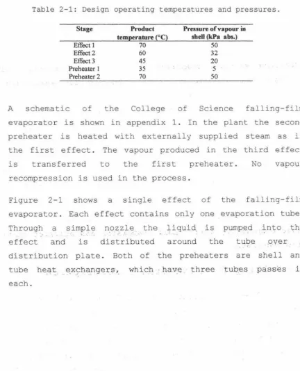
College of Science evaporator contains three effects with two preheaters and a water-jet condenser. Table 2-1 shows the design temperature and pressure operating conditions in the evaporator at steady state.

Table 2-1: Design operating temperatures and pressures.

Stage Product Pressure of vapour in temperature (0

C) shell (kPa abs.)

Effect 1 70 50

Effect 2 60 32

Effect 3 45 20

Preheater 1 35 5

Preheater 2 70 50

A schematic of the College of Science falling-film evaporator is shown in appendix 1. In the plant the second preheater is heated with externally supplied steam as is the first effect. The vapour produced in the third effect is transferred to the first preheater. No vapour recompression is used in the process.

Figure 2-1 shows a single effect of the falling-film evaporator. Each effect contains only one evaporation tube. Through effect a and simpl~ is

n_oz.zl~ _... the. liquid. is

, . ; .. pumped

distributed around the tube distribution plate. Both of the preheaters are tube heat

_..

Solution ___.

Steam---.

Evaporation Tube

Distribution

Plate~--L-J--­

.---.-....--- ----. Vapour

Condensate

Separator

Figure 2-1 A single effect of the falling-film evaporator

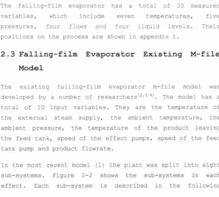
The falling-film evaporator has a total of 20 measured

variables, which include seven temperatures, five

pressures, four flows and four liquid levels . Their

positions on the process are shown in appendix 1.

2.3 Falling-film Evaporator Existing M-file

Model

The existing falling-film evaporator m-file model was

developed by a number of researchers [Z, 3' 41 • The model has a

total of 10 input variables. They are the temperature of

the external steam supply, the ambient temperature, the

ambient pressure, the temperature of the product leaving

the feed tank, speed of the effect pumps, speed of the feed

tank pump and product flowrate.

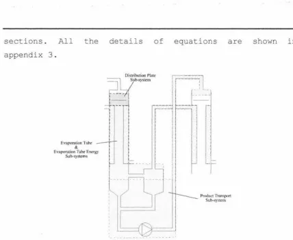
In the most recent model (1) the plant was split into eight

sub-systems. Figure 2-2 shows the sub-systems in each

sections. All the appendix 3.

Eva,x>ration Tube & Evaporation Tube Energy

Sub-systems

details of

Distribution Plate Sub-system

equations are

'

. -.. .. ~

I

I

Product Transport Sub-system

Figure 2-2: Sub-system boundaries in an effect

shown in

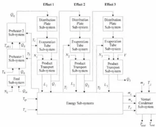
Figure 2-3 shows a diagram representation of the evaporator

Effert I Effect 2 Effect 3

Qo

i

Distribution Distribution Distribution

Plate Plate Plate

Sub-system Sub-system Sub-system

Preheater 2 Sub-system

T,

Evaporation Evaporation

Tph1 Qo Tube Tube

Sub-system Sub-system

Preheater I T3 NI N 2

Sub-system

Product Transport

To Qo Sub-system

~Q)

T

LI QI Lz _{Q2 L3} m, J

T1 _Ti

Q;.

'"c

T,P m,, Venturi

Energy Sub-systems Condenser

r,, Tc Sub-system

~111 \.enr

Figure 2-3: A diagram representation of the evaporator model

Distribution p1ate sub-system

This sub-system model s the flow of solut ion through the

distribution plat e and into the evaporation tube. The

distribution plate is considered as a mixed tank with

perforations which allow the liquid to distribute evenly

into the evaporat ion t ube.

Evaporation tu.be sub-system

This sub-system models the mass flow of the liquid out of

the evaporation tube which is obtained by performing a mass balance over the evaporation tube sub-system and the mass

of vapour produced in the evaporation tube.

Before modeling the evaporation tube sub-system two

assumptions are made:

• The fall velocity of the liquid film is assumed to be constant.

Product transport sub-system

This sub-system models the flow of product from one effect

to the next. It involves the reservoir of liquid

concentrate, the pipework connecting the effects and the in the downstream

distribution

temperature

nozzle

changes that occur through

transport system are also modeled. Evaporation tube energy sub-system

effect. The

the product

This sub-system models the heat transfer in the evaporation

tube sub-system. This includes the heat received from the

heat steam, heat lost to the surroundings and heat lost to

the downstream effect from the condensation of the vapour. Each effect is formed by these sub-systems. In addition the effects are related to the following sub-systems.

Feed sub-system

This sub-system models the flowrate of the liquid, which is

pumped from the feed tank into the first effect through the

preheater tubes. Preheater sub-system

This sub-system models the temperature of the liquid out of

each preheater. It includes the heat transfer in the

preheaters. Russe11l4l used a discrete first order

Venturi condenser sub-system

The sub-system models the suction pressure produced by the

venturi condenser and the rise in cooling water temperature

due to the condensate and vapour exhaust stream. [1]

External steam input sub-system

The sub-system models the temperature of the external steam

3

Methodology for developing the

Real-time Simulator

OVERVIEW

This chapter provides an explanation of the methodology

used for developing the real-time simulator. This

development was separated into two parts: the development

of the real-time simulator model and the development of the

SCADA control system. It begins by briefly introducing the

software used, defines the specifications of the simulator

and then describes the development procedure.

3.1 Software tools

Three software packages were used in developing the real

-time simulator model. They were Simulink, its associated

Real-time Workshop and the Microsoft Visual C++ 5.0

compiler.

The Simulink software package is provided by Mathworks cai

(Natick, Massachusetts) as a graphical environment for the

Matlab software package. Using Simulink blocks, the process

engineers can convert any M-f iles made in Matlab into

Simulink and provide a graphical representation of the

The Real-time Workshop is an additional package that can

convert a Simulink model into C code and then use a

compiler such as Microsoft Visual C to compile the

generated code into a standalone application. The application can execute in real-time with temporal

resolutions ranging from microseconds to hundredths of a

second. A pseudo- real time template was developed at Massey

University to handle tempered resolutions of hundredths to

hundreds of seconds.

The rix32 SCADA package was used as the real-time simulator SCADA control system.

3.2

Simulator Model Specifications

In its training role, the real-time simulator must match

the real plant as closely as possible in order to give

process engineers and operators a better understanding of

the characteristics of the evaporator. This includes the

development of a better graphical man-machine interface.

The real-time simulator must correctly represent the

existing M-file model. The M-files must be converted into

Simulink accurately and the steady state initial values

must be carefully selected from the existing M-file model.

In order to gain better responses (i.e . closer to the

responses of the real plant) to operator actions, some

improvement should be applied to the real-time simulator.

This includes modifications made to some of the

differential equations and adjustments made to the steady

3. 3 Methodology

The real-time simulator consists of control screens and a

Simulink model. The development of the control screens

includes two parts: drawing graphical man-machine

interfaces and building the database.

Three steps were employed in developing the Simulink model:

converting the existing model into a Simulink model,

testing the Simulink model and compiling the Simulink model

into a standalone application running along side Fix32.

The control screens were developed using the Fix32 SCADA

package. Fix32 provides the "Draw" environment that allows

development of graphical man-machine interfaces. This was

used to build control screens similar to that used in

industry.

The database for the simulation

Fix32 "Database builder". Input

was developed using the

and output blocks were

created and configured to match the variables being sent to

and from the Simulink simulation. The tagnames of these

blocks were used to match Simulink variables with the

blocks in the database.

The Simulink model was converted by choosing Simulink

blocks to perform the same actions as the m-file commands.

For example the "Function" blocks were used to perform the

calculation functions of each m-file, the "Relational

operator" blocks were used to convert the "greater", "less"

or "equal" commands in each m-file .

In each m-file, groups of commands and equations were used

of commands and equations and the relationship between each

particular function, one or more groups of these commands

and equations were converted into one Simulink sub-system.

For example, the group of commands and equations for

calculation of the product flowrate through the effect 1

distribution plate were converted into "CalcQdl" Simulink

sub-system. Each m- file was converted into one Simulink

sub-model that included a number of sub-systems. The

Falling-film Evaporator Simulink model was then completed

by connecting all the sub-models together.

After the Simulink model was completed, initial values of

the time constants and state parameters were obtained from

the trials data of the existing m-file model, some needed

to be adjusted.

After defining the initial values of time constants and

state parameters, the black box testing methodology was

employed to test the model in order to gain the initial

values of input and output variables. This was done by

setting all the inputs to their steady state values and

running the simulation until the outputs had reached steady

state. This allows the simulator to be started at steady

state each time.

After the test, the Real-Time Workshop (RTW) software from

the Mathworks was used to convert the Simulink model into C

code. This was then compiled into a stand-alone

application. As part of this process, C code files were

included to allow information to be passed between the

stand-alone application and the Fix32 database using the

4

Real-time Simulator Modifications

OVERVIEW

This chapter describes all the changes made to convert the

existing model to Simulink, create the links to the control

screens, improve simulation accuracy and robustness as well

as improve the design and performance of the control

screens. The full real-time simulator will be described

later in chapter 5.

4.1 Simulink Model Modifications

In the existing m-file model some differential equations

did not accurately represent the evaporator process. For

example the calculation of the outlet temperature of

preheater 1 and preheater 2. Also, some corrections have

been made such as the calculation of the mass of condensate

produced in the first preheater shell per residence time.

These will affect the settings of the model parameters and

the simulation results . All the other simplifications or

mistakes were corrected during development of the Simulink

model.

In order to make the Simulink model simpler and clearer,

all the constants and the system initial conditions were

put into the initial condition sub-model. This makes the

The mFromFix" driver and "ToFix" driver are also introduced

into the Simulink model. These drivers enable the Simulink

model to communicate with the control screens. Inputs from

Fix32 entered the simulation via the "FromFix" block and

the converse for the "ToFix" block.

All these changes are detailed in the following sections.

4.1.1

Preheater Sub-model modification

Two major modifications were made to the preheater sub

-model: a new differential equation was used to represent

the outlet temperature of the preheater, and the correction

of the differential equation for the mass of condensate

produced in the first preheater shell per residence time.

Changes made to the outlet temperature of the preheater

The equation ( 4 .1) listed below is a discrete first order

equation and is assumed to represent the dynamic

relationship of the preheater output temperature in the

existing m-f ile model ( TP,, ) .

( 4 .1)

Where Tph is the steady state temperature and T/p1i<l.

The term 77 phis a function of the system time constant, rc(ph)

Where t5 is the sampling time.

In equation (4.1) Tph(z) is the steady state representation

distance along the preheater tube and the time of the

liquid through the preheater tube are not being considered

as system variables. Also the liquid velocity is not being considered. For these reasons a first order dynamic was added to the equation used in the existing m-f ile model to

achieve the right type of response.

The steady state temperature for the first preheat er, 7'p1t1, is

(

_J

-Up1o1Ap1o

- U A T -T

-T phi _ T _ T - eJ d _ ''r o

+

P p1i1Cp/1QO

(4 .2)

and for preheater 2:

-l; I

- ( U A (T - T

)

J

-

""

2 .""

7' _ T _ 7• _ 7• lossph2 sph2 s a P,,i.ic,,i.Qo

p1r2 - s s p111 + e

p ph2CphQO

(4. 3)

In order t.o get a better mathematical description of the

preheater output temperature, a new differential equation

was introduced to the Simulink model to replace the

discrete first order equation. This equation was developed

by making energy balances around infinitesimal cross

sections of the preheater tubes. The temperature of the liquid in the tubes T(x,t) varies with distance along the

preheater tube and time. The following partial differential equation is produced for the temperature of the liquid in

the preheater tube. [2]

The affect of the liquid velocity on the heat transfer

coefficient was al so considered. This equation was solved

by linearisation and integral transformation in the Laplace

domain. The linearised partial differential equationis

given by the following .

( 4. 5)

x

[8T(x,t)]° =-1-[Teo -To]e-v"rr,

ax

( 4. 6)

Where the time constant is given by:

The solution of this equation is given by the following

transfer function.

( 4. 7)

This model can be extended to include the effect of fluid

velocity on the heat transfer coefficient. The following

relationship is assumed for the heat transfer coefficient.

( 4. 8)

The substitution of this into the partial differential

equation produces the following transfer function for the

( 4. 9)

This transfer function was used in the Simulink model to

replace the discrete first order function. An example of

the preheater 1 output temperature Simulink block is shown

in figure 4- 1. The left side performs difference

calculations of the transfer function and provides three

system inputs and system constants.

-u[1]/u[2]

Fen

To tTc1

Variable Transport Delay

Producl1 Sum1

Tph1

This block calculate the preheater 1 temp.

Changes made to the calculation of mass of condensate

produced in the preheater 1 shell

The old model equation (4 .10) that defines the mass of

condensate produced in the first preheater shell per

residence time does not correctly include the influence of

the heat losses. These are considered significant so a

better version derived in the following paragraphs.

dMcPhl

dt

qPhl qPhld

=

-Where q_{n 1} is heat transfer in preheater 1

qlossPhi is heat loss into surrounding

(4.10)

qn ld is heat transfer in preheater 1 with time delay

rPhl is latent heat of vaporisation

rPhld is latent heat of vaporisation with time delay

qlOSSPhl

MvPhl

McPhl

To----...,

Figure 4-2 Preheater 1

In the preheater 1 sub-system the input liquid is pumped

from the feed tank and the output liquid into preheater 2.

The heating vapour is from the effect 3 evaporation tubes.

the system are: temperature of product leaving the feed tank

(T₀) , temperature of product in the effect 3 evaporation

tube (T<,), heat transfer into preheater 1 and

preheater 1 outlet temperature (Tc.:) . The outputs from the

system are: mass of vapour produced in the effect 3

evaporation tube (M .. ) , heat loss in the surrounding

( qlossPhl), mass flow of vapour from preheater 1 (m , ) and

mass of condensate produced in the first preheater shell

(M,..F ;) .

Considering the mass balance over preheater 1, then the

mass of vapour into the preheater 1 shell i s:

The transport of vapour from the effect 3 evaporation t ube

and into preheater 1 has a time delay (r.,) . Considering this

t ime del ay and assuming const ant mass flow of vapour from

preheater 1, then the mass of vapour into the preheater 1

shell is:

Mv3(t - r.,)

=

subt racting equation (4.11) and (4.12) :

as

then

dM cP111 (t)

- - - = McP1r1(t)-McP1r1(t-r.,) dt

dM cP111 (t)

=

dJ v3 v3 e

(4 .12)

( 4. 13)

( 4. 14)

(4 .15)

By performing an energy balance over t he preheater 1 sub

to give M v3 (t) = q Phi (t) + qloss Phi (t)

rPhl (t)

( 4 .16)

( 4 .17)

The substitution of equation ( 4 .1 7) into equation ( 4. 15)

produces the following differential equation for the mass

of condensate produced in the first preheater shell per

residence time.

dMcPhl(t)

=

dt rPhl (t) rPhl( t - re)

( 4 .18)

dMcPhl qP111 + qlossPh1 qPh\d + qlossPhtd

then

₌

dt _{rPhl rPhld} ( 4 .19)

Where qloss~1ct is heat loss to the surroundings with time delay

As can be seen by comparing equation (4 .19) and (4 .10) ,

equation ( 4. 10) contains the missing term, qlossPhlct. The

Other changes made to the preheater sub-model

llh r to m"3/s1

0

0

Cale tph Calctph

t-res for qlossPh1

second level of the Preheater1 sub-model

qlossl'h1

fpreht1

Tph1

mvPh1

Figure 4-4 SQcond level of the preheater 1 Simulink sub-model

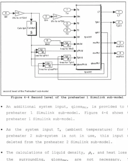
• An additional system input, qlossPhli is provided to the preheater 1 Simulink sub-model. Figure 4-4 shows the preheater 1 Simulink sub-model .

• As the system input Ta (ambient temperature) for the

preheater 2 sub-system is not in use, this input was

deleted from the preheater 2 Sirnulink sub-model.

• The calculations of liquid density, Po, and heat loss to the surrounding, qlossPh2, are not necessary. The

preheater 2 Simulink sub-model does not provide these

4.1.2

Initial condition sub-model modification

In order to make the Simulink model simpler and clearer, an

additional initial condition sub-model was provided in the

evaporator Simulink model . This sub-model includes an

"initial inputsn sub-model, a "sub-systems" sub-model and a

"constant" sub-model. These sub-models are described below.

They contain all the constants and system init ial

conditions. By collecting all the initial conditions and

constants together they can be more easily managed.

1'1 . I ,1 r •• • r,1 it.I ~ INIT INPUT (.._tt)

PM-ers···

Ta

•

37.5

Tph2 70 TO lB T1 72 T2 64 T3 42 Ql 210 Q2 200 Q3 190 L1

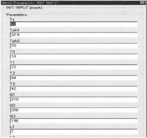
Figure 4-5 an example of initial inputs sub-model mask

• "Initial inputs" sub-systems contain all the initial

values used to calculate state derivatives. Each value is

easily changed from the block mask. An example of the

block mask is shown in figure 4-5.

• "Sub-systems" sub-model contains all the initial

calculations for each Simulink sub-model. Figure 4-6

each function block performs a difference calculation.

Each "Fromu block inputs each variables value to the

"function" block and each "Goto" block outpust the result

of the "function" block to the variables .

From3 From15 LT Pa T1 NO 00 uf1]/3.6e6 Fen

u[1]/3.6e6

Fen1

u[1)/3.6e6

Fen2

u[1]'4/3600

Fen3

u[1]'4/3600

Fen4

IJ [1 ]'4/3600

Fen5

u[1]/3600

Fcn6

Cale tph

Uhrto m"3/s

Goto1 Goto2 Goto3 Goto4 Goto5 Goto6 Goto7 Fen7 Goto

8---+§

From4 Terminator

~

8---+§

From8 Terminatoi2

~

From10 Terminator3

~

F rom 11 Terminator4

~

From 12 Terminator5

~

From 13 Terminator6

~

From 14 Terminator7

Ef-+§

Goto8 From 16 T~rminatol8

~

Constant Goto

~

B----€J

Const.ant1 Goto₁

~

0----+8

Const.ant3 Goto3

~

~

Constant5 Goto5

@---+§

Fromo Terminator6

~

Constant? Goto?

~

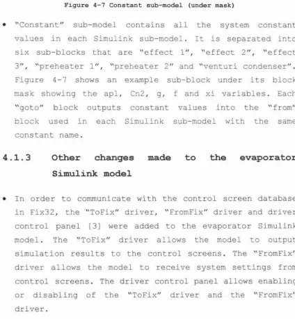
Figure 4-7 Constant sub-model (under mask)

• "Constant" sub-model contains all the system constant

values in each Simulink sub-model. It is separated into

six sub-blocks that are "effect l"

,

,

3", "preheater l", "preheater 2" and "venturi condenser".

Figure 4-7 shows an example sub-block under its block

mask showing the apl, Cn2, g, f and xi variables. Each

"goto" block outputs constant values into the "from"

block used in each Simulink sub-model with the same

constant name.

4.1.3

Other

changes

made

to

the

evaporator

Simulink model

• In order to communicate with the cont rol screen database

in Fix32, the "ToFix" driver, "FromFix" driver and driver

control panel [ 3] were added to the evaporator Simulink

model. The "ToFix" driver allows the model to output

simulation results to the control screens. The "FromFix"

driver allows the model to receive system settings from

control screens. The driver control panel allows enabling

or disabling of the "ToFix" driver and the "FromFix"

• In the existing m-file model, the unit of feed f lowrate

(Qinl is changed from l/hr to m3 /s . The conversion value

was wrong and would decrease the feed flowrate ten times.

The value is changed to 3.6*106•

4.2

SCADA Control System Modifications

The SCADA control system consists of two parts: the Fix32

database and the control screens. The Fix32 database

consists of database blocks and chains. The database blocks

include all the primary source of real-time process

information for the real-time simulator. The control

screens are graphic representation for the simulator model

which display the simulation results and allow the

simulator input parameters to be changed. In this section

the discussion of SCADA modifications is separated into two

parts, Fix32 database modifications and control screens

modifications.

4.2.1

Fix32 database modifications

The simulator Fix32 database was developed using the Fix32

"Database builder11

and included database blocks and chains.

Inputs and output blocks were created and configured to

match the variables being sent to and from the Simulink

simulation. Three types of database blocks were used in

building the simulator database. AI (analog input) blocks

were used to stall all the variable values being sent from

the Simulink model such as each effect temperature, liquid

level in each effect and flowrate for each effect. Figure

4-8 shows an example AI (analog input) block for the effect

1 outlet flowrate. The variable names were putted into "Tag

e.g. the tag name "EFFlFLOW" in the following figure was

used to match Effect 1 outlet flowrate. The names contained

in "Next Block" were used to connect with other Trend

blocks like a chain and could pass the values of these tags

into trend blocks.

Analog Input Bluet.

Tag Name~ [EFFl FLOW Ne>d Bfock: jEFF1FLOWTR

Description;j .... E--ff-c_ct_t -tl-ow- ra_t_c _ _ _ _ _ _ _ _ _ _ _ _ _

P Start Btock On Scan

Scan Time! ... r1

-~---smoothing:

112

··Hardware Specifications····

Device: ,...jS-IM _ _ _ _ _ _ _

i Hardware Options:

110 Address:

l

o

Si9MI Condltianing:

I

Engin~erin.g Units

Low limit:

1.-0-.0~----Hlgh limit: 110.29?..6

; Unft~:

l•fh

r

hlitlal Mode

r.-

. Alarms

; P EMble Atarm1ng

' Alarm Ateas: 1.-A_t_L _ _ _ _ _ _

U>w l.ow:

jo.o

Lovr.

1,...0-

.

0---, High: j1 U.292.6

2J

'

Rate of Change: Dead Band:

, Priority

lto.2s2

.

6

10:

0

1514.6

r.

r

'.. Security Areas

' ·1: [NONE 2~ !NONE 3: jNONE

OK

J

I

•••••••••••••••••••••••••••••••••••••••••••••••••n••••••••·•••••••·••••••••••••••••••••••••••••••••••••••••••••••••••••••••••-••••••••••••• ... ---···-···-·-... ..

Figure 4-8 The effect 1 outlet flowrate

AO (analog output) blocks used to stall all the variable

values being sent to the Simulink model such as pump speed

for each effect, liquid infeed temperature and infeed

flowrate . Figure 4- 9 shows an example of AO block. The same

as AI blocks, the names contained in the "Tag Namen field

were used to match Simulink variables. The names contained

Analoo Output Block

:

firl

· ... ·

· ·

... ·· ..

· ..

....

..

13

I OescriptltJ~:\ !Feed pump speed

· Hardware Specifi~i(J~s .. .

Devi:ee: .... ls_1_M _____ _

••

Hardware ~trthms:

r

. ....

.

....

Jtigh v~1ue:

~DO

I

110 Address:

10

·

...

2-)

.

Signal(:onditioning.:

·

I

~ .... -.-... -.. -... -... :,.,:,:,:,:,, ... :.:,: .. ,..,.,.-... , ... ,. ... -,:,: .. , ... .

•. E:ngi:neeting•Onjts··· ... :· .•.••...•...•....

i.~.;,.;

amn:

·

lo.oo

·

·

un

i

jloo.oo

• Units:··· ..•••

~,%---1 ... ···. . . . . .. .

hlitial Value:

\

l

o.oo

r

L

J

:,.,·.·C·:·.·:·:·.·.·,•.·C·.·.·.•C•.•,•.•,·:·.·.·.··· ····.··.·-·.·.•.·:·.·.·:·C•'.·'.·C·:·:·C··.···C,.·.·.': ····•·•·-'···•·•·•··-;._ .. , .. •.··.··:·.·.·N-"-";

[ · Ahm11s ,,. ····.. ....•.••• . · .·· ••. i

•

r

r

.

u

~:~

. <

~~

₃

.••·

·•.

~

;:

n

l

•.

·

~~

+

....

·.<> ··

... ; ... : ... ~

,i sectirliYAtea~

·

·

··

·

•

1:

INONE

. . .

2:. !NONE

!

Help

I

TR (trend) blocks contain all the variables for trend

pages. Figure 4-10 shows an example of a TR block. The

names contained in the "Tag Name" field of these blocks

were the trend block names and were used in "Next Block"

field of each AI and AO block. The names contained in

"Input Tag" field were the tag names of variable that need

to be trended from each AI and AO block.

~, Tag Name: IEFFl LEVEL T

Input Tag: IEFFl LEVEL.F _CV.

Engineering Units

LowUmit

jo

High limitj .-1-.9-7_5 _ _ _ Units:

Im

Average Compress:

Is

P Clear Buffers on startup

I

OK

Security Areas

1: !NONE

2: jNONE

3: lNONE

Help ..

I

Figure 4-10 TR (trend) block for effect 1 liquid level

4

.

2.2 Control screens modifications

The control screens are designed for the use of the

operators to change the input settings for the model and to

display the simulation results. They are desired to match

the real plant as closely as possible. For this reason they

were redrawn from industrial screens. An example picture is

\

ii;

11iriliitifill••--•

-·---·--·--·--

··

»»•·-·

·

--1

....

.

If·~

:~. ~

,_,"

_,,,;

-···•

I

[

Ti

~

·

~h

;

Il

::

,

;n

'l

:

:::::

,

®·

0

v

~

:

l!U

m

uu

I

\

, . L .,-;,:

,~:,

:~-

1

· ..

.. ;,j;;'i"·'<··:\ \

Feed watertank Pumps variable dialog boxes

Figure 4-11 An example of picture Evapma_p.odf

The control screens include seven indi victual pages, e .g.

"Evaporator A Overview", "Feed Tank", "Preheater",

"Effectl", "Effect 2", "Effect 3", and "Condensor" . In each

individual page, new pictures of feed water tank,

preheaters and effects were used to replace the existing industrial screens. New pictures of steam pipe lines; steam valve and pumps were also used to replace the existing

industrial screens.

The variable dialog boxes are used to replace the entire data link in the control screen. They can be seen from the top and the bottom of the picture shown in figure 4-12. The variable dialog boxes for the pump speed and valve position display the values of the pump speed and valve position.

pop up into the screen. The following figure shows an

example of the trend page.

~ lnl~llul10n HX VIP.W lll!lf;l £:i

5

Full Real-Time Simulator

Description

OVERVIEW

This chapter provides an explanation, with the details, of the full real-time simulator. It includes the descript:ion of the Simulink block used to develop the Simulink model, the description of the full Simulink model and the description of the control screen.

5. 1 Defining Simulink blocks in the Simulink

model

The existing m-file model provided by Nigel Russell l4l is formed by some funct:ion files known as m-f iles. These m-files are programmed in Matlab language. To convert to a graphical representation Simulink model, the m-files must be converted into Simulink blocks.

In the existing m-file model, a discrete first order equation is used to represent the dynamic function of the

Like all the variables in the Simulink model, the symbols are used to represent all the constants and the initial

condition parameters. For example, symbol 'ap' is used to

represent the pump flow characteristic constant. The constant values were input directly into the masks by double clicking each Simulink block that was contained in

the constant.mdl Simulink sub-model.

Each Simulink block used to build the Simulink model is

discussed in Appendix 4.

5.2

Simulink model description

The Simulink model consisted of the effect sub-models, the

preheater sub-model, the venturi condenser

initial conditions sub-model and the I/0

sub-models contain all the differential

sub-model, the

drivers . These

equations and

associated algebraic calculations required for each section

of the evaporator. They are connected together and show the

flow of information in the process. The evaporator effect

sub-model is used as an example and is discussed later in

this section. Other sub-models are shown in appendix 5.

There are a number of levels to the evaporator Simulink model Evap.mdl . The Simulink block diagrams in the figures on the following pages show the samples of the levels and

how the sub-models are connected together.

• The top level (Figure 5-1) shows the main inputs and

outputs of the model . It also contains the initial

:' ~ ·: : : ~ · .. : :

. ·'·· ..

...

.. /"'"1

.. ·~·:·:~·=~<~<~~~·:-:'/.'/.~~,/.~~·:<<=

...

_,_

..

,:

>----·

I

:.;.;.w/,:.rt:-:·Y/..:-'.-W/.'•Y/,:-;.;.~i:

... "'

~· ; ... , . . .. ili . ·}

. ... :r·· t.

f~

:.«<<-X<6=76~~&X4~<~xd}

Tofix

Output Driv~r

. :· ~; .:--~ ; . . .

: .. :::·:.::

Qp2..._--+<

Qin Qp3m-~~~~~

lNaporaiDr

~

Clock

Figure 5-1 Top level of the Evap.mcil Simulink model

• The second level (Figure 5-2) shows the preheater,

effects and venturi condenser sub-model linked together

and the information paths between them. It is where the

;

1

·

'

•

'

\

•

'

.... ·.~· L~

•••

...: .. "-.

. ···•

• The third level is where the information is passed into

the sub-model from the Simulink environment. An example

of this is shown in figure 5-3 for the first effect sub

-model.

t-res for q1

t-re:sfor Qd1

T•

Tph2 4 T2

5 NI

N1 feff1

Qdd1

t-res: for T1

QC

Uhr1 to m"3Js

feff1 h1 L1 Tl Qdl Qel Cpl qi Mvl 111

Cre.at Effect 1 sub-S'fSlem

"

Qd1

To Wod<spaoe

L1

t-t-i---ir--t><. 2

T1

Mv1

It-~~+--~~~-- 3 Tl1

Figure 5-3 An example of the third level of the Evap.mdl. Simulink model - Effect 1

• The lower level is where all the differential equations

and associated algebraic calculations are contained. An

example of this level is shown in figure 5-4 for the

oo(!~ Eft•c:t 1 sub-qrd.em

3

Od1

l5:

QI)

..

... +[J,JEJ

- Odl

0.1

••• ,0.1 _{.... I r+} Qpl dh1

~

0 '"+hi

-{D

c.11cH1

Oddl

Odd1 :: ... ~!' 0.1 t - - - - L I LI ...

... I : !lj

""'

~ f-+CD r--+Al dL1

-

_,,

Cl.lie 0•1 q1 _ rl

{D-rid Dt1,.,.1ti'lilt TI ... ~

_,

l

7 - qld

dT1 .._ Nl

~ Odl

..

.

..

011c0p1

'-+ Oddi qi

+[I}-- ql lit ... 2

3 : Tph2

:

LJ

"'

Tph2 _{~ T2 r#oHI} dTl1 5

4

.-i

r-+

D

M Wldot

2

=+:

"'~ • IA

I

~

Ts _{0•1 Hut11ow} dMYl

1 St.te Der!uUvu

To - - - +Tl ~oss1 > - - Ii It ::J

111 ICD--+ Tld ,,,.,

- - - +

...

,

..---T1d

,,

...

,

-

n

_,,

- - - + ... Phld

ri

lpllld ... r1

... 6

-

f l l

""''

+IA

..

'TII l'hoPhld

-0 Tl1

lptl2d thermontl ... tcal

Figure 5-4 an example of the lower level of the Evap.mdl. Simulink model

- Effect 1

Before developing each Simulink sub-model, a number of

Simulink model files are made to perform additional

calculations within the Simulink models. These Simulink

model files are used as Simulink blocks within each

Simulink sub-model.

These Simulink blocks are converted from the sub-programs

in the dynamic model. For example in these sub-programs,

the calculations of cross-section area of distribution

plate, level and volume of liquid in the Effect were the

same for the Effect 1 and Effect 2, but were different for

Effect 3. for this reason calca .m was separated into two

Simulink block diagrams, cal ca. mdl and calcaEff3. mdl. The

and the calcaEff3.mdl block was used in effect 3 sub-model.

The calctp.m was also separated into two Simulink block

diagrams, which were calctp.mdl and calctpEff3.mdl. The

calctp.mdl block was used to calculate the approximate

transport between Effect 1&2 and between Effect 2&3 in

effect 1 and effect 2 sub-models and calctpEff3. mdl was

used to calculate the approx. transport delay between

Effect 3 to output in effect 3 sub-model.

The Simulink block diagrams of these Simulink model files

are shown in appendix 5. These files include:

•

calculation

This block includes the

of the cross-sectional

equations

area on

of

the

distribution plate, area of liquid surface of the level

at base of the effect and volume of liquid in the effect

for effect 1 and 2.

• calcaEff3.mdl This block includes the equations of

calculation of the cross-sectional area on the

distribution plate, area of liquid surface of the level

at base of effect and volume of liquid in the effect

level for effect 3.

• ffcalcqO.mdl This block includes the equations of

calculation of the feed flowrate of the evaporator (Qo)

based on current plant conditions. The convert.mdl

Simulink block is used in this block to perform

calculation of saturation pressure. The densities used to

calculate the pressure are approximate densities.

• calctp.mdl This block calculates the approximate

transport delay between effect 1 and effect 2, between

• calctpEff3. mdl This block calculates the approximate

transport delay from effect 3 to output for effect 3.

• calctph .mdl This block includes the equation of

calculation of the residence time for the liquid through

the preheaters.

• convert .mdl - This block converts the temperature value

into values of a related thermophysical property, such as

saturation pressure, enthalpy or density. It also

converts the pressure value into the value of

temperature.

• calcTs .mdl - This block is used to estimate the external

steam temperature (Ts) . The external steam temperature is

technically an input variable, however, it is calculated

by the model as function of the steam controller

setpoint. The PID controller in this block is used to

adjust the steam valve position to regulate the steam

pressure in the shell of the first effect.

Evaporator effect sub-model

In an industrial production evaporator, each effect is

composed of a distribution plate sub-system, evaporation

tube sub-system, product transport sub-system and

evaporation tube energy sub-system. The Simulink effect

sub-model includes all the differential equations and

associated algebraic calculations that model these sub

-systems. Some changes are also made to perform better

simulation results.

The evaporator effect Simulink sub-model is

three sub-models, effectl sub-model, effect

composed of

and effect 3 sub-model . Most of the equations used to model

these three effects are the same with different input and

output variables. This meant that these three sub-models

have the same structures. Some differences were made while

developing each effect sub-model and are discussed later in

this section.

Effect 1 Simulink sub-model

Effect 1 Simulink sub-model contains three levels . The

first level of the sub-model is shown in figure 5-5. This

level of the sub-model is used in the second level of

evap.mdl and shows all the inputs from the outside of the

sub-model and outputs of the sub-model. There are six

inputs and six outputs as can be seen from the figure .

'Ta L1

) Ts Tl

) Tph2 Qpl

Effect 1

) T2 Mlfl

) Nl 111

) QO Qdl

Effect 1

Figure 5-5 The first level of the effect 1 sub-model

In the effect 1 m-file (feffl.m) there are ten input

variables and nine output variables that are used to model

effect 1. These inputs and outputs are applied in the

figure 5-2. As can be seen from the figure the sub-model inputs Qddl, qld and Tld are connected with the sub-model

outputs Qdl, ql and Tl through the delay block. Other two

inputs Ts and Tph2d are connected with the inputs of Ts and Tph2 through the delay blocks. All the initial conditions of these five inputs are defined in the delay block.

The main structure of the effect 1 sub-model is observed in

the third level, which is shown in figure 5-4. All the differential equations and algebraic calculations are

contained in this level and are separated into several

masked sub- systems. Each sub-system provides different

calculations. The state derivatives sub-system is used as a

sample-masked sub-system and is shown in figure 5-6. Other

masked sub-systems are shown in appendix 5.

• Cale Qdl includes the calculations of the product

flowrate through the effect 1 distribution plate (Qdl} .

• Cale Qel includes the calculations of the product

flowrate from the evaporation tube in the effect 1 (Qel).

• Cale Qpl includes the calculations of the product

flowrate out of the effect 1 (Qpl) .

• Cale Ad Al & Vl includes the calculations of the area of

liquid on the distribution plate (Ad} , volume (Vl} and the surface area of liquid level at the base of the effect 1 (Al} . The cal ca. mdl file is used to perform these calculations.

• Cale hl includes the calculations that used to clip the

height of liquid above the distribution plate in the