FOR PROPOSITIONAL LOGICS.
John Keith Slaney.
Thesis submitted for the degree of Doctor of Philosophy of the Australian National University.
in references to the bibliography and in the
ABSTRACT
I present and discuss four classes of algorithm designed as solutions to the problem of generating matrix representations of model structures for some non-classical propositional logics. I then go on to survey the output
from implementations of these algorithms and finally exhibit some logical investigations suggested by that output.
All four algorithms traverse a search tree depth- first. In the case of the first and fourth methods the tree is fixed by imposing a lexicographic order on possible matrices, while the second and third create their search tree
dynamically as the job progresses. The first algorithm is a simple "backtrack" with some pruning of the tree in response to refutations of possible matrices. The fourth, the most efficient we have for time, maximises the amount of pruning while keeping the same basic form. The second, which uses a large number of special properties of the logics in question, and so requires some logical and algebraic knowledge on the part of the programmer, finds the matrices at the tips of branches only, while the third, due to P.A. Pritchard, is far easier to program and tests a matrix at every node of the search tree.
proportion of inconsistent models (validating some cases of the scheme 'A & ~A') is much higher than might have been expected. Among the logical investigations already suggested by the
quasi-empirical data now available in the form of matrices are some work on the system R-W, including my theorem, proved in chapter 2.3, that with the law of excluded middle it suffices to trivialise naive set theory, and the little-noticed subject of Ackermann constants (sentential constants) in these logics. The formula which collapses naive set theory in R-W plus
A v ~A
is the most damaging set-theoretic antinomy known. The theorem that there are at least 3088 Ackermann constants in the logic R
(chapter 2.4) could not reasonably have been proved without the aid of a computer.
CONTENTS
Page
Introduction 1
1 The Algorithms.
1.1 A problem 12
1.2 The basic solution: Test and Change 16
1.3 Skippy 23
1.4 Cut and Guess 28
1.5 And Now For Something Completely Different 46
1.6 The method of transferred blocks 52
1.7 Conclusion to Part 1 61
2 The Output.
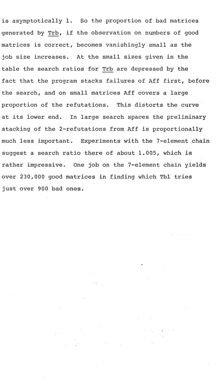
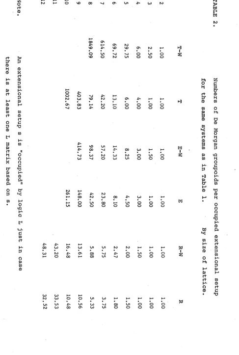
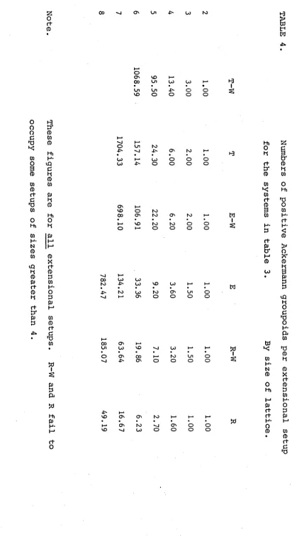
2.1 Numbers of matrices 71
2.2 Observations on the numbers of matrices 85
2.3 The logic R-W 99
2.4 Ackermann constants 117
2.5 Conclusion 142
Notes 146
INTRODUCTION
This is an investigation in two fields. Part 1 deals with the development of algorithms for the solution of the problem of computer generation of matrix model
structures for some sentential logics, and is thus
principally an essay in computing science. The project grew out of work in mathematical and philosophical logic, which subjects remain my primary interests. Part 2 of the present thesis is accordingly concerned with sentential logic, comprising an analysis of the crude output from the programs described in Part 1 and a report of some investigations suggested by that output. The two aspects of the work are by no means disjoint. The development of the algorithms was conditioned at several points by features of the logics for which matrices were required, and
conversely some of the investigations reported in Part 2 were made with the aid of a computer.
Much of the ground covered here has been very little trodden. As I report in chapter 1.1 workers in computing science have generally neglected the kind of enumeration problem I consider. Moreover the logics with which I am concerned are almost unknown to most logicians, lying well out of the mainstream of modern logic. Even relevant
logicians, concerned with logics of this class, have done little work on the system R-W which is central to my
projects, and the subject of Ackermann constants has, except for one paper which I quote, barely been noted. There has been a curious reluctance on the part of
of ideas, indeed, has been in the opposite direction, computing scientists of a theoretical bent having helped themselves to some of the deep results of recursive
function theory and the like. The lack of use of computers by logicians has, I think, at least two major causes:
the problems actually occupying workers in modern logic, in the aforementioned recursive function theory for
example, are not, given the current state of the art, helpfully programable; and the parts of logic which are
accessible to computers - elementary propositional calculus, for instance - are widely regarded as trivial and so
beneath the regard of fully qualified logicians.
Part of my claim is that the approach to computers in logic through the notion of recursive enumerability is a mistake. Computers are not good at proving theorems. They can be useful in producing crude disproofs, for instance by generating countermodels, but their better use lies in their ability to provide us for the first time in the history of logic with large amounts of quasi-empirical input data. It is for human logicians to make intelligent use of the shower of facts from the machine, whether by Baconian induction, informed conjecture or interpretation of the statistics. At the least, we have facts of a new kind demanding explanation. Why are most De Morgan monoids inconsistent (see chapters 2.1 and 2.2 below)? Why is the typical De Morgan monoid based on a lattice with few
perhaps vocabulary for a fresh approach to elementary logic. In the course of the thesis I use several notations and refer to numerous logical systems and algebraic
structures which are not generally well-known. Some definitions and conventions are now in order. Names of programming languages are given in upper case, while names of programs, procedures and algorithms are underscored. In writing out algorithms I use a version of the "Pidgin ALGOL" described by A h o , Hopcroft and Ullman in [74].
Since I do not regard "go to" as, in the pejorative sense, a four-letter word, I use it to transfer control in some places where more orthodox style would prefer more elaborate devices. My aim is always that the algorithm should be
readable.
My language for writing logical formulae has
propositional variables p,q,r,p',... . unary connectives ~ and! , binary connectives &, v, and definitions:
ADB =df. ~AvB
A=B =df. (ADB) & (BdA)
A^B =df. (A+B) & (B >A) .
In addition I use A,B,C as variables over sentences of this language. Where I use quantifiers I take x,y,z,x', etc. as individual variables and write (v) and (3v) in the standard way to represent universal and particular quantification on variable v. As may be seen in this paragraph, I generally omit quotation marks where the context makes the meaning plain. I also adopt the
(i) extreme outside p a r e n t h e s e s are omitted;
(ii) & and v bind m o r e tightly than d and = , and these
more tightly than -* and +>;
(iii) unless otherwise determined, a s s o c i a t i o n is to
the left;
(iv) a dot after a c o n n e c t i v e m a y replace a left
parenthesis who s e m a t e is to be imagined immediately
before the first f o l l owing right p a r e n t h e s i s
unmatched by an i n t e r v e n i n g left parenthesis.
T h u s :
for A-*A->B->B read ( ( (A->A)->B)+B)
for A A-*B-*B read (A-> ( (A->B) -*B) )
for (A-*B) & (A->C) ->. A-*B&C r ead ( C (A+B) & (A->C) ) -> (A-> (B&C) ) )
e t c .
M e t a l o g i c a l principles such as "rules of inference" are
w r i t t e n A, A => B
1 n
and read
if A x is a t h e o r e m and .... A^ is a t h e o r e m then B
is a theorem.
Schematic rules and t h e o r e m schemes, of course, are to
be c losed under u n i f o r m substitution.
My notation for a b s t r a c t algebras is that of the
c l a s sical first-order p r e d i c a t e calculus w i t h relation and
o p e r a t i o n constants d e f i n e d as required. I use x,y,z,x' etc.
for bound variables and a,b,c,d,a', etc. for free variables.
The universal closures of postu l a t e s should be assumed to
hold. Because the co n n e c t i v e D m a y be c o n f u s e d w i t h
implication and Vx and 3x as quantifiers.
The logics with which I am concerned are in the "relevant" group first systematically investigated by Anderson and Belnap (see their [75] for the history and more details) . The basic system T-W has the pure -> part:
a x i o m s : A->A
A+B 3->C A->C
A+B O A C+B
r u l e : A+B, A => B.
The stronger systems investigated here add in the pure -*• v o c a b u l a r y :
E-W = T-W with the assertion rule A => A+B+B.
R-W = T-W with the assertion axiom
- > -y
A A->-B->B.
T = T-W with the axiom
(A + . A+B) A-*B
E-> = T^ plus the assertion r u l e . R
- > = T^ plus the assertion axiom.
In all systems conjunction and disjunction are governed by the axioms
A&B-^A A&B-^B
(A+B) & (A+C) A+BSC A+AvB
B+AvB
Where negation is present its postulates are: A — A
A+B ~3->~A,
and in the systems T, E and R: A+~A + ~A.
TWX, EWX and RWX are defined as T~W, E-W and R-W respectively with the addition of "excluded middle":
Av~A.
Where L is any of the six systems, "L" without a subscript has -*■, &, v and "L, " has & and v; "L " has -> as its
T ->
sole connective.
The fundamental algebraic structure to model logics of this kind is the Ackermann groupoid, a quintuple
< S , < , o , t> where :
S is a set, < is a partial order of S , ° and + are dyadic operations on S, teS, and:
t°a = a (left identity)
a < b ^ c»a < c<>b Cmonotonicity) aob ^ c ° a < b+c (residuation) .
A model of logic L is a homomorphism from the sentence algebra of L into an Ackermann groupoid, the operation modelling the connective -*. Formula A holds in model m iff t ^ m(A). A class of Ackermann groupoids
(a°b)°c < a « (boc) (a°b)°c < b°(aoc). For T add to these a°b < (a°b)°b.
For E-W add the postulates for T-W^ and a < a°t,
For E add all four of these. For R-W add to the basic structure a°(b°c) = bo(aoc) and
a°b = b°a,
and for additionally a < a°a.
The positive logics have models obtained by making < in Ackermann groupoids a distributive lattice order and also replacing the second (monotonicity) postulate by
a« (bvc) < (aoc) v (b<>c) which gives
a°(bvc) = (a°c) v (boc) and
(avb)oc = (a°c) v (b°c).
The extra postulates corresponding to particular systems are unaffected. For negation introduce a complement operation, , subject to the postulates
a = a
a°b < c =* a°c < b.
3x V y (y ^ x y £ a & y < b)
aAb =df. lx Vy (y ^ x ° y < a & y < b)
similarly avb =df. ix Vy (x < y ° a < y & b < y) aA(bvc) = (aAb)v(aAc)
a = a
a £ b => b < a.
The quadruple ( S, < , , t > I call an ex t e n s i o n a1 s e t u p
,
and a De M o r g a n g r o u p o i d resulting from it by the addition of ° and -> with their postulates is said to be b a s e d on the extensional setup. A De morgan groupoid satisfying all the postulates corresponding to the system R is calleda De M o r g a n m o n o i d in the standard literature on relevant
logic. The terminology is taken from various sources including Belnap, Dunn, Meyer and Routley,
The concept of a matrix model structure for a propositional logic is at least as old as truth tables, and has been fostered in its modern form mainly by many valued logicians following the pioneering work of
Lukasiewicz and Post. It is now standard to regard such a structure as a triple <M,0,D> where M is a set, 0 a set of operations on M and D £ M. The operations in 0 are correlated 1-1 with the connectives of a language L and
a m o d e l of L in the structure is a homomorphism with
respect to this correlation from L into <M,0>. A sentence
h o l d s in a model iff it is mapped to a member of D by that
iff all theorems of that logic are valid in the matrix, and to be c h a r a c t e r i s t i c for the logic iff exactly the theorems are valid. For present purposes, however, a stronger notion is required, since we must be able to recognise matrices which satisfy a given logic. I therefore require the set
D of designated values to be closed under my canonical rules of inference adjunction and detachment. That is to say I am only concerned with f i n i t e s t r o n g m o d e l s in the sense of Harrop (see [65]). Harrop's f i n i t e w e a k m o d e l s, in which the rules of inference preserve validity but not designation are of less interest, if only because they are not in general recursively enumerable. Matrix models have a variety of uses, in disproving nontheorems, in showing independence of axioms, in demonstrating the non-equivalence of formulae (as in the chapter on Ackermann constants
below) and in proving consistency, for example. They have also been used to establish syntactic properties of
ACKNOWLEDGEMENTS
Where I have consciously used others' works, whether published or not, I record the fact either in my
text or in references to such works, listed at the end of the thesis. I should, however, record my more general
indebtedness to those who have contributed less specifically but equally importantly to my thinking. The greatest debt is to Dr. R.K. Meyer who supervised my work and who has contributed not only the idea of the matrix-generating project but also many of the formal and philosophical points making up the theory of the logics with which X am here concerned. My other supervisor, F.R. Routley, was responsible for arousing my interest in paraconsistent logic, which underlies the comments on R-W in chapter 2.3 below. For their discussion of such logical matters I
am also indebted to Professor N.C.A. da Costa of the University of Sao Paulo, and to Dr. G.G. Priest of the University of Western Australia. The background to my algebraic work on the relevant logics is dominated by
Professors N.D. Belnap and J.M. Dunn, with additional input from A. Urquhart, Routley and Meyer inter multis. My
thanks go also to the members of the Australian National University logic group, among whom especially is
Dr. E.P. Martin who collaborated with me for a while when I first began to use the computer to find matrices and who has acted as a sounding-board for my wilder ideas
for a while. His contribution to my present subject will be obvious from the ensuing pages. In particular the algorithms described in chapter 1.5 are entirely his. Among my Departmental colleagues outside the logic group
I owe most to Professor J.J.C. Smart who, though my tastes in logic I fear are not his, has never failed with
encouragement for my work. By no means the least of my
debts is to Alice Duncanson, the typist of the present work, who cheerfully tackled a difficult manuscript, making the rough places plain; any residual unintelligibility is the fault of content alone.
Chapter 1.1 A problem
In many cases problem-solving algorithms are
required to return a single answer to each problem: there is generally a unique shortest route for a travelling
salesman, for instance, and the next move in a board game, though not uniquely determined by the rules, is uniquely selected. Sometimes, however, a problem has many solutions, all equally wanted. If, for example, we want to know what words can be constructed from a given set of letters it will not do for an algorithm to stop short of generating
them all; if the problem is to find all the mappings of a given set onto itself which are isomorphisms with respect to some imposed structure then there is no preferred one which counts as the "best" solution. The present thesis
is concerned with a problem in the latter category.
The general description of the multiple solution exhaustive search problem is:
given: a finite set {a ....a }; i n a set S of finite sets;
a function V: {a ....a } -- *■ S;
i n
an open sentence (or "postulate") P(xi....x^); define: a s e t u p is a function f with domain { a ^ ^ . a }
such that for 1 < i < n, f(a^)e V(a^);
the s e a r c h s p a c e is the set of setups;
problem: to find and accept all and only the good setups from the search space.
In actual cases the problem can be made more tractable by lettinq a ...,a be the variables x ..,,x which occur in P and letting V assign to each variable a set of possible values. Then a setup is simply an assignment of possible values to the specified variables, and P can be regarded as
a c l o s e d sentence. If each member of S is of cardinality
k then there are kn setups in the search space, so in general exponential bounds on time complexity should be expected.
The reference points a x....a may be organised in such a way as to simplify P, of course. Where they are variables they might well be structured in arrays for easy reference, and this device underlies the special type of multiple solution exhaustive search considered here. I take the variables a,....a to have canonical structures
i n
based on the first M+l natural numbers, 0....M. There may be integer variables, taking particular numbers as values; there may be Boolean arrays of the form [0:M,....,0:M] which take as values arrays of members of {True,False};
there may be integer arrays of the form [0:M,....,0:M]
taking as values arrays of members of Intuitively the Boolean arrays represent r e l a t i o n s defined on {0....M} and the integer arrays represent o p e r a t i o n s on the same set. Such setups are recognisable as matrix representations of abstract algebras of small sizes.
such algebras, though the adaptation is easier in some cases, such as that of Pritchard's SCD (chapter 1.5), than in others, such as that of the Cut and Guess of chapter 4. They were designed, however, to solve a more specific problem, described in more detail in the
appropriate places below. This concerned matrix model structures for sentential logics, and particularly for logics of the "relevant" group. The choice of logics was a result of historical accident, but turns out quite
felicitous, since these logics have the right numbers of matrices of small sizes to be reasonably investigable
(see chapter 2.1) and have postulates of sufficient
complexity to make recognition of a good setup a nontrivial matter. The fundamental connective of the logics specified
in the Introduction above is the implication and the hard problem is to find matrices for it. Under the
influence of Polish notation Meyer (see chapter 1.2) dubbed the integer array representing the connective 'C' and this convention has stuck. No easy way is known of looking
for satisfaction of the prefixing and suffixing axioms -C[C[x,y], C[C[w,x], C[w,y]]]
C[C[x,y], C[C[y,z], C[x,z]]] - which makes the problem interesting.
concentrated on enumerating some permutations of a
sequence or certain integers (such as primes) for example, rather than on rich algebraic structures. There is
occasional mention in the literature of problems
encountered in enumerating semigroups, which is getting near home, and I have found one paper (Plemmons [67]) on generating finite algebras in general. I cannot imagine that techniques for enumerating latin squares are going to be directly useful here, but one area in which some
intellectual capital has been invested is the investigation of ways of finding - or avoiding - isomorphisms on a given structure and this may indeed provide my research programme with some input. True, the going results are given in
*
terms mainly of the queens problem , rotations of the n-cube and the like, but there is growing interest in
applying them to generating semigroups, partial orders and so on, and once abstract structural similarities between the problem classes become evident there may be something of value to the enumeration problem for families of
Ackermann groupoid.
Chapter 1.2 The basic solution: Test and Change
In November 1976 Meyer began looking for all the small matrix models of the system E_^. His idea was to have a file of such matrices for the systems in which he was interested, partly for sundry purposes such as
disproving the occasional nontheorem or distinguishing between non-equivalent formulae and partly for perusal, to help in gaining a "feel" for this or that system. In the three years since then we have indeed begun to make use of these matrices, as reported in part 2 of the present work. The problem of efficient generation of the matrices, however, has become interesting in its own right and has been pursued for its own sake and for the insight it gives into computing methods.
The algorithm Meyer proposed for generating good setups from the search space as defined in chapter 1.1 requires that the elements a 1....a be placed in a linear order, which can be represented by the numerical order of their subscripts, and that the possible values of each a^ be ordered too: I shall write v^(a^) for the j-th member of V(a^). The basic algorithm runs:
for i 1 until n do f (a^) «- v 1 (a^) ; ! This is the initial setup,
f is a function variable ; Test: if P(f(ax)....f(a )) then accept f ; Change: for i «- 1 until n do
if V(A^) is of cardinality j then
else
f (ai) v 2 (a^J
b e g i n
f(ai> " v j+i(ai> *
go to Test
end
In the special case considered by Meyer the array to be filled with values is a 3x3 matrix. The outline of his algorithm is:
Declare: integer array C[0:2,0:2];
Initialise: for i 0,1,2 do f o r j «- 0,1,2 do C [ i , j ] +■ 0 ;
Test: if C validates then accept (C); Change: fo r i 0,1,2 do fo r j +- 0,1,2 do
if C[i,j] = 2 then C [i,j] 0
el s e b e g i n
CCi,j ] + C[i,j] + 1;
go to Test
e n d
This original Test and Change routine, which
School FORTRAN", produced 147 matrices for in a little
over 6 seconds of runtime. Having disposed of the 3x3 problem Meyer, under the impression that he had banished hard work from logic for ever, revised his program to search the 4x4 space. The new program ran for some minutes without
producing anything at all, so he did some elementary
arithmetic. Calculating that about 4.5 times as many steps are involved in generating and testing a 4x4 matrix as are involved at 3x3 and multiplying 4.5 by 6 seconds by 416 divided by 39 he concluded that the new job should take approximately 69 days'*". Accordingly he set out to improve the algorithm.
Meyer's technical contribution was to note that the search space can be defined much more efficiently than in the naive way. All familiar logics with an implication connective, , have some useful properties. Define a < b in the algebra represented by a matrix m as m(a-*b)eD where D is the set of designated values. Now < is a weak partial order
-a < -a
a < b , b ^ c ^ a ^ c
- and only in matrices with utterly superfluous values is it not the case that
a < b , b ^ a ^ a ^ b .
Any partial order can be embedded in a total order, so we may take the ordering of the elements represented by
0 1 2 3 0 D u u u 1 S D u u 2 S S D u 3 S S S D
S - {0,1,2,3}
D = designated values u = undesignated values.
Nothing is lost by assuming all designated values to be higher numbers than all undesignated ones, since clearly every matrix is isomorphic to one of this kind. With the designated values closed numerically upward there is no need ever to test the rule of detachment, since if A -*■ B takes a designated value then A takes a value not numerically greater than that of B, whence if A takes a designated value so does B.
There are now three search spaces for the 4x4 problem, determined by the three choices of D:
D # matrices
{3} 2,985,984
{2,3} 4,194,304
{1,2,3} 331,776
total 7,512,064
At the rate suggested by my earlier experiment (see note 1) this job should run in about 12% minutes, on the given
hardware, which is quite acceptable. The time complexity of the algorithm, though, is still dictated by Test and Change to the extent that a similarly projected runtime for the 5x5 problem is in the region of 80 years!
computers to matrix model structures followed the development of a FORTRAN program Tester by N.D. Belnap and D. Inser.
Tester arrived in Canberra in 1976. It is a highly user- interactive program designed to test sets of postulates read in at runtime against matrix sets also entered at runtime. The details are of no importance for the present work but the program remains useful in everyday logical research after four years and Belnap is to be credited with having sparked interest in the nest of problems
associated with computing and matrices. The only anticipation of their work known to Meyer and Pritchard (see chapter 1.3 below) was a paper by R.T. Brady (Brady [76]) on the question of generation of matrices satisfying sets of postulates.
Brady describes some procedures for initialising the search space for designated and undesignated values which foreshadow the space-priming techniques of my later programs (see
chapters 1.4 and 1.6 below). The type of job Brady considers is slightly different from that to which I have addressed myself, as he wants a program to accept, as Tester does, an arbitrary logic and search space read at runtime. This flexibility should be expected to come at the cost of some efficiency, for it is generally the case that the more problems an algorithm can tackle the less efficiently it tackles each one.
One unsettled debate raised by the Brady paper and continued in Meyer and Pritchard [77] is between the
Any language used for this progam should preferably be a machine language with mnemonics and indirect addressing. If a language such as FORTRAN is used, the program would be less
efficient and hence the range of problems it could tackle would be smaller.
Brady [76] p.248 Pritchard replies:
Finally, we feel it necessary to take strong issue with Brady's claim that a matrix finding program should be written in an assembly (machine) language. Time is much better invested (we
present our results as evidence!) in improving the efficiency of a matrix finding a l g o r i t h m rather than that of a p a r t i c u l a r m a c h i n e
-i m p l e m e n t a t -i o n . A high-level language can then
be used to quickly obtain a reliable, efficient and portable algorithm.
Meyer and Pritchard [77] p.10. In evaluating these contrary claims it must be remembered that the two authors are addressing rather different
problems. Brady is not much concerned with the details of a matrix finding algorithm, but rather with those of rendering an arbitrarily presented problem of the type tractable. And it is true that a program which starts by devising a piece of code to test the postulates and loads this into the core first will run markedly faster than one which, like Tester, represents each postulate as a string of numbers and tests by manipulating the
subscripts. Pritchard is certainly correct, however, in claiming that the algorithm is much more important than the implementation. The naive search problem is dominated
/ _ 2 \
by the 0(nv ) imposed by the number of possible matrices, while the speed-up due to assembler implementation is
little better than linear, and thus in the long run
can do in a matter of minutes; there are many which a program ten times as fast could not do in a week; there are not many jobs between these two groups. Improved algorithm design must precede improved implementation, for only a better algorithm than the early ones can ever hope to take on the investigations at up to 30x30 considered in the sections on Ackermann constants below. A few pages back we met the jump between 12% minutes for the 4x4
Chapter 1.3 Skippy
By early in 1977 Meyer had realised some of the limitations of the naive Test and Change algorithm and in an effort to improve it enlisted the help of P.A. Pritchard, then a student in computing science at the Australian
National University. Pritchard's contributions to the subject have dominated it ever since. The first major advance due to Pritchard resulted in the algorithm I call Skippy and incorporates a device used in one form or another by all subsequent solutions.
I define a r e f u t a t i o n of a setup f as a subset f of f such that for no good setup g is it the case that
f
S
g. A refutation is a k-refutation iff its cardinality is k. Consider now an assignment of values to variables in the suffixing axiom which shows a particular matrix C to be bad. The assignment gives an undesignated value toC[C[i,j], C[C[j,k], C[i,k]]]
and in the course of discovering this we have to "look up" at most four cells of C: we need values for C[i,j],
C[j,k], C[i,k] and C[C[j,k], CCi,k]]. If
therefore we reject the matrix C because of this assignment we are rejecting it on a 4-refutation at most. Its
be changed. Clearly any matrix differing from C in at
most the first i-1 places will contain the same refutation, and so all matrices can be skipped until the first one to change the i-th cell. A bad matrix will typically yield
several refutations, so we should choose the best; the best is the one whose least cell (i.e. the earliest in the change order) is later than the least cell of the rest, so that we may maximise the number of useless matrices skipped before the next try.
Let us now think of the cells of C as given in a linear order - the order in which they are changed - and write C. for the i-th cell in this order. Where R is a
l
refutation of C we write RC for the set of indices of cells used in R. Recall that R is a set of ordered pairs each consisting of a cell and its value. The procedure m i n (X) delivers the least of a set X of numbers, and max(X) likewise the greatest. I sometimes write the parameter here as (a,b) instead of ({a,b}). Now the procedure Test delivers an integer "index" being the index of the first cell to be changed, and Change begins the search for the next matrix from C. , . There are n cells,
index
Procedure Test
begin i a "found refutation" is the subset of C
actually looked up in a falsification of a postulate ;
for each found refutation R do
c index max (index, min(R 1)
P r o c e d u r e Change; b e g i n
fo r i 1 until n do
if i < index or C. = M then 0
e l s e b e g i n
C . C . +1 ;
i l
index 0 ;
go to E
end ;
finished true ; E : end ;
Now the algorithm proper:
finished «- false ; index ^ 0 ;
f o r i * • 1 until n do 0 ;
w h i l e not finished do
b e g i n
Test ;
if index = 0 then accept the matrix ; Change
end
The Skippy algorithm given above is substantially as given in the unfinished paper by Pritchard and Meyer
that the choice of order can made a considerable difference to the time taken, but failing to find any general principle for determining a p r i o r i the best such order. I have given the algorithm for the "idiot" search as I did for Test and Change. As before, its efficiency is greatly improved by allowing only designated values on the main diagonal and only undesignated ones below it.
My contribution to Skippy was to complicate it somewhat by adding a device for changing the change order as the job progresses. The basic observation here is that at the start of the job, when all cells have their initial values, the change order can be selected quite arbitrarily, though once some cells have non-initial values their order becomes fixed. The generalisation of this observation is that if at any time during the loop there occur two cells adjacent in the change order both of which hold their initial values then at that time those cells can be regarded as
unordered relative to each other, though they are ordered relative to any non-initial cells before or after. This fact is important when there is a string of cells with their initial values one of which is the cell C. , from which
index
the change proper is to start, for maximal efficiency is
gained by assuming to be the last cell in this string. Accordingly, in the case where C£ncjex holds its initial value
it is moved up the change order as far as the next non-initial cell. The other constraint is that it must not displace any other cell used in the selected refutation, of course,
since C. , is to be the l e a s t cell used. Other cells used index
way to make room for it. A simple algorithm to implement the idea uses a Boolean flag ’swop,is,on' and an integer pointer 'ptr';
swop. is.on false ;
f o r i +• n s t e p -1 u n til 1 do ,
if C. does not hold its initial value l
then swop. is.on false
e l s e if swop.is.on and was used in the refutation
then b e g i n exchange Ck and in the change order ;
ptr + ptr-1
end
e l s e if not (swop.is.on or was used in the refutation)
then b e g i n swop,is.on «-= true ;
ptr 4- i end ;
This is inserted at the start of the Change procedure.
The device of changing the change order as the job progresses can make an important difference in execution times, as may be seen from the figures given in chapter 1.7 below. It was never used much for serious programs, though, because the much more efficient algorithms described in
chapter 1.5 and 1.6 became available very soon after its invention. The pleasing thing about it is that it provides a way for Skippy to optimise for itself its change order,
removing the need for a great deal of quasi-empirical research, and answering one of Pritchard and Meyer's open questions
Chapter 1.4 Cut and Guess
The problem which brought me into contact with the matrix-generating programs concerned the logic RWX (see
Introduction above and chapter 2.3 below). I particularly wanted to see some of the matrices which split RWX from
the logic R which is properly stronger. This posed two serious problems. In the first place the extant programs searched for -* matrices only, while RWX and R are full logics with rich structure: conjunction, disjunction and negation are all present as well as implication. The
additional connectives demanded new thoughts on organising the search. In the second place, RWX matrices which fail R are rare. There are only 7 pairwise non-isomorphic RWX matrices of size 4x4 or less, only one of which fails R. Here it is:
Hasse diagram 3
negation
0
1
*2 *3
3
2
1
0
implication
0 1 2 3
0
1 *2 *3
3 3
1 3
2 3
0 3
This matrix actually shows a good deal. It is based on a Boolean algebra, and hence shows not only that RWX is weaker than R but that CRWX is weaker than CR and even that KRWX is weaker than K R . 2 By itself, however, one matrix does not tell much of the story. There are just
5 matrices of sizes up to 7x7 which split the two systems; one of these is the 4x4 Boolean monoid just given and another
Hasse diagram
0 1 2
*3
*4 *5
5 4 3 2 1 0
-y 0 1 2 3 4 5
Q 5 5 5 5 5 5
1 Q 4 4 4 4 5
2 0 1 3 2 4 5
* 3 Q 1 2 3 4 5
*4 0 1 1 1 4 5
*5 0 0 Q 0 0 5
Thus I required the machine to search in the 8x8 search space at least - an impossibly vast task without using the richness of the logic's structure to impose tight constraints on the subspace actually searched. As an indication of the rarity of model structures for these logics, note that from all search spaces up to 10x10 - i.e. naively
10 1 0 0 + 9 8 1 + ___ + 39 + 24
possible matrices - fewer than 700 yield pairwise non isomorphic model structures for R.
The first program designed to help in generating these matrices was due to E.P. Martin and called (rather euphemistically) Fast. Fast required a search space
specified in full in an input file and worked by applying to it a fairly crude Test and Change loop. It tested only the suffixing axiom
-B->C "►. A->3 . A-*C
- assuming the rest of the R-W postulates to be written
into the search space. That this can be done will be proved later. The significant innovation, Martin's technical
possible much greater flexibility in the matter of the search spaces which can be represented and tested, and I now use it in all my matrix-finding algorithms.
Fast need not be detailed here; the ALGOL program Tnc given in chapter 1.7 below is very similar and may be examined to see the workings of the idea. The method of preparing the search spaces, though is very important and should be illustrated. Consider the job of looking for 8-element models of R-W, and think of these given
algebraically, but with as the principal operation instead of °. Now clearly the general case is far too big for Test and Change, so we must devise a series of smaller jobs and execute these in turn. As noted in the Introduction above, an algebraic model of R-W is based on an extensional setup, or quadruple <S, <, -, t> where S is,
for the moment, constant as the set {0,1,2,3,4,5,6,7}, < is a distributive lattice order on S, - is a De Morgan complement on S and teS. We may, for the 8-element
De Morgan extensional setup case, assume that (i) < is embedded in the numerical order;
(ii) if a is numerically greater than t then t < a; (iii) a = 7-a if a ^ a . 3
Hasse diagram complement 7
> 6 0 : 7 t = 1
T 5 1 : 6
O 4 2 : 5 designated values:
<> 3 3 : 4
Y 2 1/2,3,4,5,6,7
o 1
0 undesignated value:
One generally useful property of the complemented structures I consider in this thesis is contraposition: a+b = b->a.
In the case of this chain contraposition means that we need only construct half a matrix since the cells below the
top right-bottom left diagonal will be mere mirror-image copies of those above. The Change component of our program can easily allow for this by changing the cell C[7-b,7-a] every time it changes C[a,b], and running its recursion through the top left triangle of cells only. The initial search space is thus:
(x) (0 < x) so in particular 0 < 7 -* a 7 < 0 -> a by permutation
and 7 < a -> 7 by contraposition, assuming 0 = 7. t -> a = a and a -* f = a where f = t.1* And a derivable rule:
a < b, c < d =>■ b c < a -> d.
From 7 < a -* 7 we have 0 -*■ a = 7; from t -* a = a we
have 1 -*■ a = a; the rule of affixing gives us the important principle:
A f f . a < b, c < d => Vxe[be]3ye[ad] x < y £ Vxe[ad]3ye[bc] y < x.
Here I use [ab] to designate the set of possible values of C[a,b]. Applying all this to our initial search space we are able to remove some of the values to leave:
0 1 2 3 4 5 6 7
0 7 7 7 7 7 7 7 7
1 0 1 2 3 4 5 6
2 0 0 12 123 1234 12345
3 0 0 0 123 1234
4 0 0 0 0
5 0 0 0
6 0 0
7 0
Not all the jobs are so simple to prepare. When the order is not a chain the complexities increase, and in most cases the first effort will not reduce the numbers of matrices below the 100,000 or so which can easily be tested. Some more principles useful for cutdown include: Perm: a < b+c => b < a+c
RWP: aA(a^O) = 0 (this only holds of RWX) ft: f < t => a+b < b->a.
At the time when I was using Fast I did not know about RWP (the second R-W paradox - see chapter 2.3 below) or ft, though the latter is easy enough to derive:
suppose f < t
then a+f < a->t
but a+t < t->b ■>. a->b so a->f < t-*b ■*. a-*b
but a->f = a and t-^b = b so a < b •>. a->b
so a < a->b->-b (by contraposition) so a->-b < a->b (by permutation)
i . e . a+b < b->a (by contraposition).
suppose a ->b =5 7 i.e. 7 < a->b
then a < 7^b (by permutation) so a < b->-0 (by contraposition) but bA (b-^0) = 0 (RWP)
so either b = 0 and b = 7, or b->0 = 0 and a = 0, since 0 is not. meet-reducible.
In any case, if a-*b = 7 then aAb = 0. In that it appeals to RWP, this derivation requires that the extensional setup be such as to validate excluded middle.
Consider, then, the search space for R-W matrices on the 8-element chain with five elements designated - i.e. as before but with t = 3. Applying the above principles we eventually reach:
0 1 2 3 4 5 6 7
0 7 7 7 7 7 7 7 7
1 0 3456 3456 3456 6 6 6
2 0 12 345 345 5 56
3 0 1 2 3 4
4 0 01 012 012
5 0 01 012
6 0 01
7 0
Here there are 4 3x35x25 = 497,664 possible matrices, which makes the job a little too big for comfort. The
0 1 2 3 4 5 6 I 7
0 7 7 7 7 7 7
r
7 7
1 0 3 345 345 6 6 6
2 0 12 345 345 5 56
3 0 1 2 3 4
4 0 0 012 012
5 0 0 012 4+1 = 0
6 0 0
7 0 2 2x3 7 = 8748
0 1 2 3 4 5 6 7
0 7 7 7 7 7 7 7 7
1 0 456 456 6 6 6 6
2 0 12 345 345 5 56
3 0 1 2 3 4
4 0 1 12 12
4+1 =
5 0 01 012
6 0 01
7 0 2 5 x 3 5 = 15,5
The total for the two jobs is now 24,500 setups: a
twentyfold reduction in job size at the cost of roughly doubled overheads and increased risk of human error.
Fast did indeed produce some results pertinent to my original project concerning RWX and R, but there were
1. F a s t was rather specialised; a program to search for models of a greater range of logics would be an
improvement.
2. The preliminary paperwork was tedious and time-
consuming - more so than was justified by the results. 3. Garbage in: garbage out. Mistakes are very easily
made in the preparation of the search spaces, and render the results meaningless.
4. The piecemeal approach was logistically inefficient; I kept losing the bits of paper.
5. After 8x8 I was going to have to search at 9x9 and 10x10, where problems 1, 2, 3 and 4 could be expected to be amplified exponentially.
The obvious solution was to program the initialisation and cutdown of the search space.
My first attempt to do so produced a program called Mag (Matrix generator). The input to Mag was an extensional setup in the form of a partial order table, complement
table and choice of t, and the output all the R-W matrices on that setup. A simple variant which also applied
aA(a+b) < b
b e g i n
r e a d in d a t a o n < S , <, t > ;
i n i t i a l i s e : set [ab] as t h e d e s i g n a t e d (undesignated)
v a l u e s if a < b (a J b) ;
set t-*a = a; set a->M = 0>a = M ;
if e x c l u d e d m i d d l e h o l d s t h e n for each a ,b
do if a A b ^ 0 then [ aO ]-*-[ aO ] - (b } ;
c u t d o w n : a p p l y p r i n c i p l e s l i k e A f f to s q u e e z e i m p o s s i b l e
v a l u e s o u t of th e s e a r c h s p a c e ;
p r e t e s t : if t h e n u m b e r o f m a t r i c e s r e m a i n i n g in the s p a c e is l a r g e then
b e g i n
g u e s s : f i n d a c e l l < a , b > w i t h as f e w v a l u e s as p o s s i b l e ,
g i v e n t h a t it ha s at l e a s t 2 v a l u e s ;
p u s h th e c u r r e n t s p a c e o n t o a s t a c k w i t h the
l o w e s t v a l u e r e m o v e d f r o m [ab] ;
r e m o v e f r o m t h e s p a c e all v a l u e s o f [ab]
e x c e p t t h e l o w e s t ;
go to c u t d o w n
end ;
t e s t : r u n T e s t a n d C h a n g e on a n y m a t r i c e s r e m a i n i n g
in the s e a r c h s p a c e ;
pop: if t he s t a c k is n o n e m p t y then
begi n
p o p the l a s t s t o r e d s p a c e f r o m th e s t a c k ;
r e w r i t e th e c u r r e n t s p a c e as this p o p p e d o n e ;
go to c u t d o w n
ENTRY
read in
data
stack empty matrices
left many
EXIT
split cell
other way split a
cell
test
change set up
search space
apply cutdown principles
printup
M a g
"The number of matrices is large" was determined
empirically to mean "the number of matrices is greater than about 600", so a cutoff point was set at 600 for determining whether to "guess" at the value in some cell and cut the search space again or to test the remaining matrices. The Test and Change loop was taken from Fast.
The power of Mag comes from the Guess component, which divides the search space. Choosing a cell with only
2 values if possible is to try to keep the search tree
balanced, as well as to achieve maximum effect from each cut. In the example given earlier the first division reduced the job size by a factor of 20; in larger jobs it is not unusual for a single Cut and Guess (more accurately Guess and Cut given that English "and" is not commutative) to reduce the search space by a factor of 1010 or more.
Later versions of Mag produced a series of programs under the title Bigmat (Big matrices), the first of which was compiled in May 1979. The improvements incorporated
in Bigmat were sometimes fairly trivial - it gave a choice of systems, of fragments of systems and of output formats, for instance, and could take many extensional setups based on many partial orders in one execution - but some were of more significance. Mag had used an idiotic Test and Change loop, while more efficient ones were on the market at the time. Bigmat incorporated the device Skippy.
was eliminated by an application of a cutdown principle. The cutdown loop, too, could be made more efficient, as suggested below.
Bigmat successfully investigated my chosen logics up to the limit of the number of matrices which could reasonably be held on an output file. Thus it produced all De Morgan monoids (R matrices) up to 11x11, R-W up to 10x10, E and T up to 8x8 and E-W and T-W up to 7^7. These were matrices for the full logics. I have not been much concerned with fragmentary systems, though my programs now are equipped to investigate them. Another significant use of Bigmat was in finding De Morgan monoids on large De Morgan lattices of sizes up to 18x18 and 20x20. These helped in the search for Ackermann constants (see Chapter 2,4 below), where an exhaustive search of one particular 14-element
structure proved most fruitful. We have been able to view structures of much greater size and complexity than was possible with Fast or Mag, and while some of the results have surprised us it must be said that we have begun to outrun ourselves in that we lack the techniques to analyse
such complex data or to pick out from it that which is of interest. Presumably manipulation of such large model structures will have to be by computer since most 20x20 matrices are machine-readable at best, being unintelligible
to the human eye.
b e g i n
r e p e a t cut false ;
for each cutdown principle p do
for each cell ( a,b) do
for e a c h possible value, x, in [ab] do
if C[a,b] = x is impossible because of p then
begin
cut out x from the possible values of <a,b> ; cut true
end
u n t i l not cut
e n d
A typical cutdown principle is Aff (the affixing rule): Aff: for i 0 until M do f o r j < - 0 until M do
begi n
fo r k 0 until i do for 1 Q until M do
if k £ i and j < 1 then
begin
for each possible value, x, in [ij] do
if ~3y (yeCk'l]&x<y) then b e g i n
drop x from [ij]; cut true en d ;
for each possible value, y, in [kl] do if ~3x(xe[ij]& x<y) then
b e g i n
drop y from [kl]; cut 4- true end
end
Remember that unless otherwise stipulated < refers to the imposed partial order, not numerical order. The loop is a search for 1-refutations only.
This early Cut and Guess routine was inefficient in several ways, and most significantly because the
recursions on i,j,k and 1 in the above loop, for instance, run through all the values, meaning that every pair of cells related by affixing is examined on every pass. In fact
there will be no values to drop unless one of the cells in the comparison has been cut either on the present pass through the loop or on the last (the arbitrary cut due to splitting a cell counts as the 0-th pass), Thus we find that efficiency is improved, especially on large jobs, by keeping a record of the cells cut on each pass, and only looking for further cuts where the record indicates their possibility.
The most time-efficient version of Cut I have treats it as a recursive procedure. The key insight here is that the cuts pursuant to a division of a cell are all in cells predictably related to that cell. Thus for instance if c is removed from [ab] and there remains no de[ab] such that d < c then there may be failures of affixing in cells <x,y> where x < a and b < y, while if there remains no de[ab]
such that c < d then there may be affixing failures between <a,b> and <x,y> if a < x and y < b; no other failure of affixing can be caused immediately by that
particular cut. Analogous methods pick out the values and cells to which a cut may spread by the other cutdown
worth giving in full, and in general the programmer must use knowledge of logic and algebra to devise both the cutdown principles and the procedures for most efficient discovery of likely places to find derived cuts.
In broad outline, then, the recursive Cut procedure reads:
P r o c e d u r e Cut (x,y,z); v a l u e x,y,z;
b e g i n
drop z from Cxy]; ! This may involve recording the cut, setting flags, etc. ;
f o r e a c h cutdown principle, p, do
f o r ea c h cell <a,b> related to <x,y> so that p applies do
f o r e a c h ce[ab] do
if p applied to <x,y> rules out c as a value of < a ,b ) then
Cut (a,b,c) en d .
In its latest implementation this Cut procedure occupies some 300 lines of rather densely written ALGOL, which is a measure of its complexity. It does simplify the logic of the main program greatly, of course. The drive down of the search now reads:
w h i l e the number of matrices remaining in the space is
large do for s o m e value, x, in a cell <a,b> with more than one value do
Cut (a,b,x).
problem: a solution by "divide and conquer". Before
this will work, however, we have to put the tests for the actual axioms tried in Test and Change into the cutdown loop. This is not difficult. Consider the case of the suffixing axiom:
a+b < b->-c •*. a->c.
This does not easily yield a direct cutdown principle because of the nested arrows, but where [be] and [ac] are unit sets the values of b-*c and a+c are fixed, so we have:
fo r i + - 0 until M do
f o r j ■*- 0 until M do
fo r k + ■ 0 until M do
i f [jk] and [ik] have just one member each then hegi n
Cut from Cij] any value not < some member of [ j-*k, i-*k];
Cut from [j+k,i->k] any value not > some member of [ij]
end .
Thus by the time only one matrix is left in the search space all instances of the axiom will have been tested. Other axioms are similarly easy to incorporate.
As detailed in chapter 1.7 below Cut and Guess in this form is moderately efficiently. It is very
Thus my first instinct, to use Cut and Guess to prime the search space and some other method to do the fine search, was right. The other problem faced by Cut is its recursive procedure form is core usage. It takes a noticable amount of core just to load a procedure as big as Cut, and
additionally every time it is entered 10 or 12 new
variables are declared to avoid feedback problems. Thus on very large jobs, where calls 100 deep are not uncommon, this adds a significant burden to core usage, already running high to accommodate the search space and other arrays, and has sometimes pushed me over limits. It is often possible to buy space at the expense of time, but this is rather unsatisfactory. Cutdown as a mere loop is not subject to the same problem and has been used to
Chapter 1.5 And Now for Something Completely Different,
The title of this chapter is that of a paper by Pritchard dated October 1978 in which he outlines an algorithm for finding matrices by a radically new method. The algorithm works by repeatedly dividing the search space S in response to refutations found. With a search space S we associated a matrix C by setting
C[a,b] = min(S[a,b]).
Thus at any time the matrix being considered is that formed by assigning each cell its lowest available value. The matrix is tested (and if good then accepted) and a
refutation of it, as defined in chapter 1.3 above, selected, A good matrix counts as a refutation involving all the cells
Now consider a
< x ,a > b a d .
one of which lacks x a at C 2 :
Notice, though, that <y,b> occurs in both spaces, so if we merely make these changes we may try the same matrix twice. The answer is to keep the singleton of the "bad guy" only at one of the cells while cutting the other:
with more than one possible value. 2-refutation involving cells C 1 and
S x , y ,z a , b,c
We should now search two subspaces, at C and the" other of which, lacks
Sj y , z
S 2 x,y,z
a,b,c
Sj y,z a
s
2
x,y,z b,cHere e v ery pair of v alues e xcept <x,a> o ccurs in just one of
the subspaces. An a n a l o g o u s device w o r k s for large
refutations. Suppose < x , a , i > is a 3-r e f u t a t i o n of the setup
S x , y ,z a,b,c
Then we shall split to give
c 3
if j fk
y,z
x,y, z
x , y , z
b , c
a,b , c
i
i
jfk
P r i t chard's a l g o r i t h m implements the search d e p t h-first
via a stack of triples e a c h r e p r e s e n t i n g a cell to be divided,
the v a l u e s taken out and w h e t h e r the b r a n c h thus represented
has yet been searched. The d e t ails of stack man i p u l a t i o n s
are not important except for the note that they are v ery
simple and so can be p e r f o r m e d e x t r e m e l y fast. In a later
note d a t e d June 1979 P r i t c h a r d gives the a l g o r i t h m in the
! S. denotes the j-th member, under a standard order, of the set ;
Vi C. S ^ ; finished «- false ; 1 i
r e p e a t stop «- false ;
Test C ; ! This gets a smallest refutation R ; if C is good then accept C ;
if I Rj = 0 then stop true
else b e g i n ! R = (r1 ,...,r } ;
extend the search tree with
and take the leftmost branch end;
if stop then b e g i n
back up the search tree ;
if we reach the top then finished true end
u n til finished.
In the 1979 note are four criticisms of this
order. Smaller refutations are more significant than larger ones, and a more efficient search results if they are higher in the tree. This can be brought about by inserting
refutations into the stack not necessarily at the end but above any larger refutations provided that these do not involve any of the values at cells (including cells with only one value) used in the given refutation. Thus the
search tree is modified dynamically as the search progresses. Pritchard's second criticism is a minor matter of making the stacking procedure more elegant. The third and fourth are more important. It will often be possible to process several refutations from one test, where such refutations are all disjoint. This applies especially to 1-refutations, which of course are bound to be disjoint. Such mutiple processing
should be done, or the next matrix will contain a refutation we already knew about, which is inefficient. The last point made in Pritchard's note is in the form of a question: in general what is the b e s t refutation (of a given size) to choose. This is difficult, and perhaps no generally right answer exists. One suggestion of Pritchard's is to choose refutations involving cells with fewer possible values rather than those with more. In comparing two refutations it may be possible to devise a generally adequate answer, but the
complexities which arise when comparing two sets of refutations may lead to a preference for "heuristic" rules of thumb.
Still, the algorithm is simple in outline,
by the number of values at cells - i.e, 0(.n3log n) where n is the number of values, for there are 0 (n) values at each of the n 2 cells. On prepared search spaces such as those put out by Cut and Guess there will be many fewer values, of course.
At the time when I received a copy of the SCD algorithm (August 1979) Pritchard had not implemented it, so there was no empirical detail on its performance. My first reaction was to write a version of Fast (see chapter 1.4 above) to search prepared 8x8 spaces by SCD. What I implemented was a very crude first attempt at the algorithm, incorporating none of the suggested improvements and not even searching for a smallest refutation of each matrix but processing the first one found. This program was moderately efficient, but no faster than the later versions of Bigmat. It should not be concluded, though, that SCD is in any sense a failure. In the first place, the investment of some
time in incorporating into my little program some of the known improvements to the algorithm must result in an order of magnitude drop in runtimes. In the second place one of the most exciting facts about SCD is that nothing in its construction turns on the nature of the algebraic structures for which it is to search, so it should be of very general application to problems in the classes defined