Some problems in kernel curve estimation

(1)

I

Some problems in kernel curve

estimation

DATE

by

Ann Margaret Cowling

A thesis submitted for the degree of

Doctor of Philosophy of The Australian National University

1,

,,·

.I

_{May 1995}

(2)

Corrigenda

In the text below, the numbers in brackets refer to the page and line number (page, line).

• ( 4,8) Add the following sentence in brackets at the end of the first paragraph on page 4: "(Marron and Wand (1992, p729ff) give a number of further objections to higher order kernels.)"

• (5,10) Change hopt to hAoPT· Add the following immediately after equation (1.4). "Note that hAoPT minimises the asymptotic MISE rather than the actual MISE; see Marron and Wand (1992) for some comparisons of the minimiser of the actual MISE and asymptotic MISE which show that the difference may be large in some practical situations."

• (5,-9) Add the reference Cao et al (1994).

• (5,-14) Change the sentence "This produces h2, then j(r+2), h3 and finally j(r) ." to "This produces h2, then j(r+2), h3 and finally j(r); see for example Wand and Jones (1995, p72)."

• (7, Section 1.3) Move the 5th paragraph of this Section, beginning "A point

t

...

"

to immediately before Corollary 1.1.

• (7, Corollary 1.1) Change the second sentence to the following: "For any boundary point x

= qh

where q E [0, 1), provided h - 0 and nh - oo as n - oo

bias

{}(x)}

= -f(

x)

1

K(u)du+ O(h)

.

"

• (8,16) Add the reference Muller (1993).

• (18,-8) Add at end of sentence, "where f

= r(0) is the estimate

of the scale parameter r based on the original sample X.

• (20,9) Change "the convergence of U(x)" to "the convergence of suprT(x)". • (28,5) Replace the first sentence of the paragraph with "Local polynomial kernel estimators gained renewed attention following the papers of Stone (1977) and Cleveland (1979). Recent work of Fan (1992, 1993) has shown that they have a number of advanta-geous properties, including minimax optimality properties and desirable MSE properties."

• (28,10) Add the reference Wei and Chu (1994).

• (30,8) Add the following as a new paragraph after the first paragraph on page 30 " Note that while G is monotone, a polynomial interpolant may be non-monotone. In addition, a polynomial fit may behave erratically in places. These matters are discussed further in Section 2.4.1."

• (30,9) Change "Note" to "Note also".

• (33,-10) Change the sentence beginning "Let h,..., ... " to "Let h,..., const.n-1₁₍2_r+I), and let m be of larger order than n2r/(2r+1), and of smaller order than n{2r/(2r+1)}+11, where 0 ~ TJ ~ 1/(2r

+

1)."

(3)

• (35,1) Move the headings for Section 2.4 and 2.4.1 to the top of the page, above Figure 2.1.

• (43,7) Change the sentence beginning "Particularly at the ... " to "The left-hand end shows the trend in intensity at the beginning of the period when the accident rate was very high, and the right-hand end shows how current safety policies are working. In both cases it would be of interest to know whether the intensity is increasing or decreasing, but reflection cannot provide an answer."

• ( 43,-11) Add at the end of the second paragraph of Section 2.4.3 "The cross-validation score function used was

CV(h)

= fo

1

~(x)2

dx

+

2

I:

Li(Xi)

'

where ~(

x)

is the estimate of the intensity constructed using both the real data and the pseudodata, and

I:;

~-i(Xi)

is the sum over the sample points of the intensity estimates at each sample point, Xi, where each estimate is constructed using the all the sample points except the ith, and the pseudodata."

• (59,1) Replace the sentence beginning "The manner in ... " with "The manner in which our univariate algorithms should be modified is straightforward.'

• (61,-7) Change hopt to hAoPT·

• (74, Section 3.4.1) Change all occurrences of hopt to hAoPT·

• (74,11) Before "The roughness ratios ... " add "The chosen sample sizes are typical of the sample sizes which arise in many practical settings and were chosen so that the conclusions drawn from the simulations would be applicable in such contexts."

• (76,-3) Change the sentence beginning "Moreover, the peaks ... ' to "While the confidence band is consistent with a monotonically decreasing intensity, examination of a number of bootstrap simulations suggests that the peaks around x

=

0.2 and x

=

0.7 may be real features of the curve; see Cowling et al (1995)".

• (78-82, captions) Change each occurrence of hopt to hAoPT·

• (125, References) Add the following references:

Additional References

Cao, R., Cuevas, A., and Manteiga, W. G. (1994). A comparitive study of several smooth-ing methods in density estimation. Comp. Statist. Data Anal. 17, 153-176. Cowling, A., Hall, P., and Phillips, M. J. (1995). Bootstrap confidence intervals for the

intensity of a poisson point process. J. Amer. Statist. Assoc. submitted.

Fan, J. (1993). Local linear regression smoothers and their minimax efficiencies. Ann. Statist. 21, 196-216.

Marron, J. S. and Wand, M. P. (1992). Exact mean integrated squared error. Ann. Statist. 20, 712-736.

Muller, H.-G. (1993). On the boundary kernel method for non-parametric curve estimation n ar ndpoints. Scand. J. Statist. pages 313-32 .

[image:3.609.19.594.19.759.2]

(4)

I

11

I

Ii

11

II

Declaration

I hereby declare that this thesis describes my own work, supervised by Professor Peter Hall. A portion of it has been submitted for publication in papers jointly with him and Dr M. J. Phillips from the University of Leicester, who visited the Centre for Mathematics and its Applications in 1994.

Ann Cowling

(5)

ii

I

Acknowledgements

I am deeply grateful to Professor Peter Hall for his supervision. Although he was

extremely busy, his door was always open and he gave generously of his time. His

help has been invaluable.

I would like to thank the School of Mathematical Sciences and the ANU for their

financial support.

My thanks go also to the other postgraduate students, members and visitors of

the Statistical Sciences Program in the Centre for Mathematics and its Applications

for their cheerful company, friendship and support.

(6)

II

ll

I

_{Related Publications}

The following papers have been submitted for publication from the work in this

thesis:

Cowling, A. and Hall, P. (1994). On pseudodata methods for removing bo

und-ary effects in kernel density estimation. J. Roy. Statist. Soc. Ser. B, under revision.

Cowling, A., Hall, P. and Phillips, M. J. (1994). Bootstrap confidence regions for

the intensity of a Poisson point process. J. Amer. Statist. Assoc., submitted.

(7)

Abstract

In this thesis, we present solutions to two problems in kernel curve estimation. First

we give a new method for reducing the boundary bias of kernel density and intensity

estimators. We apply this method in our second contribution, the development of

bootstrap confidence bands for the kernel estimator of the intensity of an

inhomo-geneous Poisson point process.

The thesis is divided into three chapters. In the first we give an introduction to

kernel density and intensity estimation, review the traditional methods of boundary

bias correction, and briefly present bootstrap methods and their use in constructing

confidence bands for kernel curve estimates. This chapter provides background and

motivation for our iater work.

In Chapter 2, we describe our new method for reducing the boundary bias of

kernel estimators of arbitrary order. The proposed technique involves generating

pseudodata beyond the support of the density

f

, then using

the pseudodata as well

as the original data in the usual kernel estimator, thereby boundary-correcting the

estimator. The pseudodata are simple to generate: they are formed using linear

combinations of the order statistics of the sample, with co-efficients that vary

ac-cording to the order of the kernel. We show that the kernel estimators produced in

this way have optimal orders of bias and variance throughout the estimation interval.

Our method is applied to simulated data, and optimal pseudodata generation rules

are proposed. We compare the performance of our method with that of traditional

methods, and find that our method outperforms the traditional optimal boundary

kernel method when

f'(O)

>

0. Finally, we compare pseudodata, reflection and

boundary kernel intensity estimates for the classic coal mining disaster data set

(8)

given in Jarrett (1979).

In Chapter 3 we develop theory and methods for calculating confidence bands for the intensity function A(x) of an inhomogeneous Poisson process. Unlike previous

researchers, we treat the Poisson process as genuinely non-stationary rather than as a

Cox process. This requires us t'o derive the asymptotic distribution of j( x) - E j( x ). Our work complements previous work on point estimation, as well as contributing new results on confidence regions.

There are numerous ways of applying the bootstrap to develop confidence bands

for E

i

We describe methods based on several different bootstrap resampling

al-gorithms and a number of approaches to pivoting. We remove edge effects using

our pseudodata estimator, and correct the confidence intervals for bias, producing

intervals for .A. We demonstrate the effectiveness of these different approaches both

theoretically and numerically using simulated data. Lastly, we discuss the intensity

of the coal mining disaster data in the light of our confidence bands for .A.

(9)

µ'

Technical Lemmas

(11)

List of Tables

1.1 Parallels between order statistics and Poisson processes 26

2.1 Boundary slopes of densities used in simulation study 38

2.2 Comparison of two-point rules for

f'

(O)

<

0 51

2.3 Comparison of two-point rules for

f'(O

) >

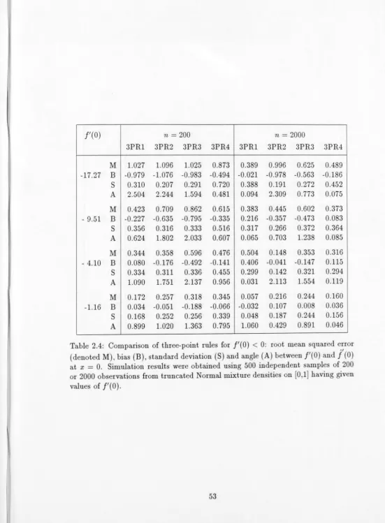
0 52

2.4 Comparison of three-point rules for

f'

(O)

<

0 . 53

2.5 Comparison of three-point rules for

f'

(O)

>

0 . 54

2.6 Comparison of boundary correction methods for

f'

(O)

<

0 55

2.7 Comparison of boundary correction methods for

f'(O)

>

0 56

3.1 Comparison of coverage probabilities of confidence bands for

>.

using

smoothed bootstrap with different bandwidths . . . . . . 80

3.2 Observed coverage probabilities of confidence bands for

>.:

bias co r-rection by undersmoothing with recommended bandwidth choices . . 81

3.3 Observed coverage probabilities of confidence bands for

>.

:

bias

cor-rection by undersmoothing with suboptimal bandwidth choices . . . . 82

(12)

List of Figures

1.1 Usual kernel density estimate: fixed kernel construction . . 1.2 Usual kernel density estimate: moving kernel construction 1.3 Boundary kernels for x

=

0, 0.2h, 0.4h, 0.6h 0.8h, h 1.4 Boundary kernel density estimate

1.5 Reflection kernel density estimate 1.6 Cut-and-rescale density estimate .

1.7 Cumulative number of coal mining disasters: 1851-1962 2.1 Location of pseudodata: factors influencing sign of X(i) 2.2 Empirical quantile function

G

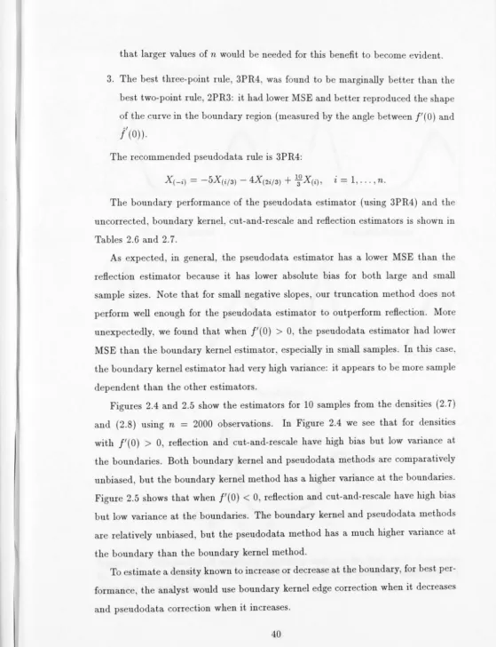
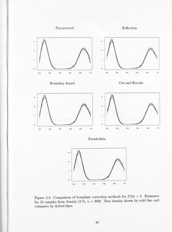
and extensions at boundaries 2.3 Densities used in simulation study . . . .. . . . . 2.4 Comparison of boundary correction methods for

f'

(0)

>

0 2.5 Comparison of boundary correction methods for

f'

(0)

< 0

2.6 Intensity of coal mining disasters: comparison of boundary

reflection and pseudodata estimates . . . . . . . . . . . . . .

3

6

9

10 11

12 22 35 36 39 41 42

kernel, 44 3.1 Bootstrap confidence band for intensity of coal mining disasters 76 3.2 Comparison of confidence band construction methods: bias correction

by undersmoothing with recommended bandwidth choices . 78 3.3 Comparison of confidence band construction methods: bias correction

by undersmoothing with suboptimal bandwidth choices . . . . . . . . 79

(13)

Chapter

1 Concepts of kernel curve

estimation

1.1 Introduction

Non-parametric curve estimation techniques make no assumptions about the func -tional form or distribution of the data. The one assumption concerns the smoothness of the curve: typically, that it has at least two bounded derivatives.

In kernel curve estimation, the estimate at a given point is constructed using only local information: it is constructed from data values that lie in a neighbourhood of the point. To ensure that the estimate is consistent, as the sample size increases the neighbourhood must shrink in such a way that the points become dense in the neighbourhood. As only local information is used in the construction of an estimate, the convergence rate of these estimators is quite slow.

In applications, the support of the curve to be estimated is often known to be bounded on one or both sides. The smoothness assumption renders the kernel estimator unable to reproduce a discontinuity such as may occur at a boundary, and so the usual kernel estimator is much more biased near the boundaries than in the interior. For small and moderate sample sizes, a substantial portion of the support of the curve can be adversely affected by boundary bias. A number of different methods of reducing this bias have been suggested.

(14)

Non-parametric smoothing is an especially useful tool for exploratory analysis,

as it may reveal structure that would be missed by imposing a parametric model.

With the addition of a confidence band around the smooth curve, an unexpected

structure can be assessed as either likely to be a real feature of the underlying curve

or only an artifact of the sampling process.

In this thesis, we will be concerned with kernel estimation of density and Poisson

intensity functions. However, the same principles apply, perhaps with modifications,

to the estimation of regression curves.

The remainder of this chapter reviews in more detail the relevant aspects of kernel

curve estimation. In Section 1.2 we present some basic concepts of kernel density

estimation which are used throughout the thesis. The principal traditional methods

of reducing boundary bias are given in Section 1.3. We review Poisson processes

and define the kernel estimate of the intensity function in Section 1.4. Section 1.5

introduces the bootstrap and describes how it is used to construct confidence bands

for kernel curve estimates. In the final section, Section 1.6, we motivate and outline

the research detailed in Chapters 2 and 3.

1.2 Basic results in kernel density estimation

Kernel density estimation has attracted much research interest since the publication

of the pioneering papers of Rosenblatt (1956) and Parzen (1962). Some recent books

include Devroye and Gyorfi (1985) developing the 11 theory of density estimation;

Silverman (1986), the classical introductory work; Scott (1992) on multivariate

den-sity estimation; and the new introductory text of Wand and Jones (1995) covering

fundamental aspects of kernel estimation and many of the areas of research interest.

The traditional (see Silverman (1986, pl5)) and conceptually natural view of the

construction of the kernel density estimate is as follows. Suppose that X1, ... , Xn

is a random sample from an unknown continuous distribution with density f. A

kernel function K spreads equal probability mass through neighbourhoods centred at each Xi, with width depending on the bandwidth h. The estimate is the sum of the heights of these kernels.

(15)

"'

0

"'

0

-0

0

-2

' '

,,

'

-

---

::::.;.>~

liii

i

T-

T1

rTi

_iti~;;;;:i::~~>

--1 0 2 3 4

Figure 1.1: Usual kernel density estimate (dashed) for data from a truncated Normal density (solid). The estimate is the sum of the kernels (dotted) centered at the data points. Bandwidth h

=

1.65.

This 1s illustrated m Figure 1.1 for a small simulated data set consisting of seven points from a truncated Normal distribution. This data set is used through-out Chapter 1 to demonstrate various kernel estimates and their construction. In practical applications, many more observations would be used: we use only seven observations here for clarity in the figures.

More formally, the usual kernel estimator of

f

is n

}(x)

=

(nht1

I:

_{K {(}_{x -}

_X

_;

₎

_/

_h},

i=l

where h is the bandwidth, and K is an rth order kernel satisfying

I

1

j

uiK(u)du

=

O

~

1

0

if i

=

0

if 1::;

i::;

r - 1, if i

=

r.

(1.1)

(1.2)

It is obvious from ( 1. 1) that

j

has the same differentiability properties as K, so that the order of the kernel r is the number of bounded uniformly continuous derivatives that must be assumed for f.

The bias and variance of

j

are given in the following theorem, which is easily proved using Taylor expansion; see for example Silverman (1986, p39).

(16)

I

Theorem 1.1 If f has r bounded uniformly continuous derivatives and K satisfies

the conditions in ( 1. 2), then provided h - O and nh - oo as n - 00

'

bias

{}(x)}

var {}(x)}

(-1r _!_ /<i, hr f(r)(x)

+

o(hr) r!

(nht1 f(x)

j

K2(u)du

+

o{(nht1 }.

(1.3)

Clearly the bias of

J

can be reduced by using a high-order kernel. However, kernels of

order greater than two have negative side lobes, which may result in negative density

estimates in places where data are sparse. Therefore, to ensure that }( x) ;?_ 0 for

all x, second order kernels are generally used in practice.

The bias of the estimate can also be reduced by using a smaller bandwidth h,

but this leads to a noisy estimate

J

with local detail masking global features of the

sample

(f

has high variance). If his large,

J

is smoother but the global features are

dampened

(f

has high bias and low variance). The bias, then, can only be reduced

at the expense of variance and vice versa, with the bandwidth h determining the

ratio of (squared) bias to ~ariance.

The choice of the bandwidth his perhaps the central issue in kernel estimation.

We shall discuss bandwidth choice briefly here as it is not addressed elsewhere in

this thesis.

Although in some circumstances it may suffice to choose the bandwidth by eye,

automatic methods of choosing a bandwidth are generally preferred for their

ob-jectivity and relative time efficiency. The automatic methods minimise an error

criterion, usually integrated squared error (ISE) or mean integrated squared error

(MISE), where ISE =

J(f

-

f)

2 _and_MISE₌ _E

_J(f

_-

_!)2

. See Jones (1991) for a

discussion of the relative merits of these criteria.

Least-squares cross-validation, independently proposed for use in density

esti-mation by Rudemo (1982) and Bowman (1984), minimises the ISE. More precisely,

the cross-validatory bandwidth is that value of h which minimises

/

A2

-1""'

A

f - 2n ~ f(-i),

l

an unbiased estimate of (ISE-

J

/2)

,

where f(-i)

=

{(n-l)h}-1 I:i# K {(x-Xi)/h},

the kernel stimate off constructed using all the data points except Xi. The chosen

(17)

I

bandwidth is consistent but Hall and Marron (1987, 1991) have shown that the relative rate of convergence of methods minimising the ISE cannot be less than

n-1/10 whereas the relative error of methods based on minimising the MISE can be

reduced to n-1_/2_.

As

MISE

j

E {}(x) - f(x)}2dx

/ [bias{}( x)} ]2 dx

+

j

var{}( x)} dx

,...., (r!r2 K-2 h2r

j

f(r)(x)2dx

+

(nht 1

j

K2(u) du ,

it is minimised by

(1.4)

Perhaps the most popular of the bandwidth selection methods targeting MISE

are plug-in methods, which are based on using an estimate of f(r) in (1.4); see

for example Scott et al (1977), Park and Marron (1990) and Sheather and Jones (1991). The determination of j (r) involves a chain-like procedure: typically, an initial bandwidth h1 is chosen and used to estimate f(r+4). This produces h2, then

j(r+

2

), h₃ and finally

j(r).

An obvious question is how the number of iterations should be chosen.

Empirical comparisons of various bandwidth selection methods using simulation are given in Park and Marron (1990), and Park and Turlach (1992). Comparisons based on real data sets are given in Sheather (1992). As yet no definitive reco m-mendations for an optimal bandwidth selection method can be made.

The bandwidth need not be constant throughout the estimation interval.

Vari-able bandwidths depending on the estimation point x, the data points Xi or both

have been proposed and studied; recent works include Jones (1990) and Hall (1990, 1992b).

Just as an "optimal" bandwidth can be found by minimising the MISE with

respect to h, an "optimal" kernel can be found by minimising the MISE with respect

to K, subject to the constraints (2.2). The optimal second order kernel, for example,

(18)

I

.,,

0

" 0

M

0 ()

N ()

0

0 0

-2 -1 0 2 3 4

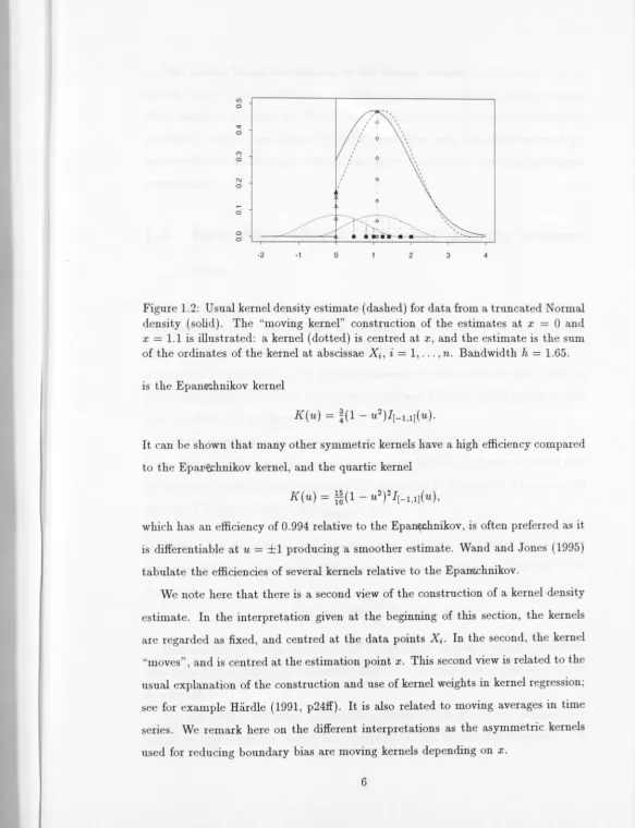
Figure 1.2: Usual kernel density estimate (dashed) for data from a truncated Normal density (solid). The "moving kernel" construction of the estimates at x

=

0 and

x

=

1.1 is illustrated: a kernel (dotted) is centred at x, and the estimate is the sum of the ordinates of the kernel at abscissae Xi, i = 1, ... , n. Bandwidth h = 1.65.

is the Epanechnikov kernel

K(u)

=

¾(1 -

u

2

_)I[-i

_,

1

](u)_

It can be shown that many other symmetric kernels have a high efficiency compared

to the Epan~hnikov kernel, and the quartic kernel

K(u)

=

~!(1-

u

2

)2J[-i,1

](u),

which has an efficiency of 0.994 relative to the Epan~hnikov, is often preferred as it

is differentiable at u

=

±l

producing a smoother estimate. Wand and Jones (1995)

tabulate the efficiencies of several kernels relative to the Epantchnikov.

We note here that there is a second view of the construction of a kernel density

estimate. In the interpretation given at the beginning of this section, the kernels

are regarded as fixed, and centred at the data points Xi. In the second, the kernel

"moves", and is centred at the estimation point x. This second view is related to the

usual explanation of the construction and use of kernel weights in kernel regression;

s e for example Hardle (1991, p24ff). It is also related to moving averages in time

senes. We remark here on the different interpretations as the asymmetric kernels

used for reducing boundary bias are moving kernels depending on x.

[image:18.610.15.598.16.776.2]

(19)

I

II

I Ii

I

The movmg kernel construction of the density estimate at the point x is as

follows: centre a scaled kernel at x, and take as the estimate the sum of the ordinates

of the kernel at abscissae Xi. Whilst this construction can be clearly illustrated for

an isolated point x, see Figure 1.2, it does not allow such clear illustration of the

construction of the estimator over the full range of x values as does the fixed kernel

construction.

1.3 Boundary effects in kernel density

estima-tion

When the support of f is bounded, the usual kernel estimator (1.1) performs poorly near the boundary. The variance is the same size, o{(nht 1

}, in the boundary

regions as in the interior, but the bias is much greater. More specifically, as x

approaches a boundary b,

f

(

x) tends increasingly to underestimate

f

(

x), until at

the boundary under the usual consistency conditions, E

f

(b) l'V ½J(b), as can be seen

from Corollary 1.1 to Theorem 1. 1.

The underestimation at the boundary is illustrated in Figure 1.1 on page 3. This

figure also shows that kernels centred at points in the boundary region extend past

the boundary making

f(

x

)

>

0 beyond the support off. Thus when

f

has bounded support,

f

is not a density since fsupp(f)

f

=/-

1.

Corollary 1.1 In addition to the conditions of Theorem 1.1, assume that K and

f

are supported on [-1, 1] and [O, 1] respectively. Then, provided h ---t O and nh ---too

as n ---t oo,

bias

{f(x

)}

= -

f(

x

)

i

1

K(u)du

+

O(h).

Because the bias in the interior is 0( hr), edge effects dominate the global asymp

-totic behaviour, influencing bandwidth choice in cross-validatory or plug in methods

for example.

We will revi w the main traditional methods which have been proposed for

boundary bias reduction, and in the remainder of this chapter and Chapter 2, will

(20)

assume without loss of generality that

f

has compact support

[

O

,

1 ].

We will

fur-ther assume that K has com pact support [-1, 1] as otherwise the whole estimation

interval

[O

,

1 ]

would be subject to boundary effects.

A point t whose location in

[

O

,

1 ]

does not depend on n is not informative for

studying boundary behaviour since as n - t oo, h - t O and so t will eventually

become an interior point. Therefore, for studying boundary behaviour we consider

a sequence of points x(n) which have the same relative location in a boundary

interval for all n: x(n) = qh or x(n) = 1 - qh, with q E [O, 1). Only the correction methods at the left boundary will be described; corrections at the right boundary

can be obtained analogously.

1.3.1 Boundary bias reduction techniques

Boundary kernels

Gasser and Miiller (1979) proposed usmg different kernels, called boundary

ker-nels, in the boundary regions for kernel regression. They developed the theory in

Gasser et al (1985), and suggested that boundary kernels could also be employed

for correcting edge effects in density estimation.

We must take the moving perspective of the construction of the estimator when

discussing the boundary kernel method as boundary kernels vary according to the

estimation point x. For a boundary point x

=

qh, only the interval [-1, q) of

the support of K is mapped into

[

O

,

l

].

The boundary kernel at x, Kq, is defined

as a modification of the interior kernel K, which has support [-1, q) and satisfies

the moment conditions of the interior (1.2). It is desirable that Kq should depend

continuously on q and that Kq - t K as q - t 1.

The boundary kernel estimator is

if x E [0, h);

otherwise.

The definition of boundary kernels ensures that the bias of

}BK

is of the same order

in the boundaries as at interior points.

(21)

0

0.0 0.2 0.4 0.6 0.8 1.0

Figure 1.3: Boundary kernels based on the Epanichnikov kernel as given in (1.5) at x

=

0, 0.2h, 0.4h, 0.6h, 0.8h, h. Bandwidth h

=

0.4.

Suppose that the Epanichnikov kernel is used in the interior. For the left bound-ary region, Gasser et al (1985) propose the 2nd order polynomials

(1.5)

where c0 , c1 and c2 are constants depending on q such that

and

Figure 1.3 shows these kernels for various values of q.

Using the quartic kernel in the interior, Hall and Wehrly (1991) employ 5th order

polynomial boundary kernels based on the quartic kernel:

The coefficients c0 and c1 are obtained by solving

and

These kernels are defined so that Kq(-1)

=

0. Although similar in general outline

to the Gasser, Muller and Mammitsch kernels, the Hall and Wehrly kernels are

smoother as they are differentiable at u

=

±1. The Hall and Wehrly boundary kernel estimate for the simulated data set is shown in Figure 1.4. Note that fsupp(f)

fBK

-/-

1.

(22)

"'

0

"'

0

-2 -1

·.,

't

1\ I ' :

' '

' ·,

I r, ,' [\

,' 6 ' 0 0

0

;

.... ···;·--: __ ....

:·

~.

·. ··-..

-i, '• "" • •. --·•_{. . .}_~-- ····•···· '" ' ---'-"----===

··...[ ____

.~---0 2 3 4

Figure 1.4: Boundary kernel density estimate ( dashed) for data from a truncated

Normal density (solid). The construction of the estimates at x

=

0 and x

=

1.1 is illustrated: a kernel (dotted) is centred at x, and the estimate is the sum of the ordinates of the kernel at abscissae Xi, i

=

1, ... , n. Bandwidth h

=

1.65.

Although boundary kernels reduce boundary bias to the appropriate order, they

are not strictly positive; see Figure 1.3. This means that the boundary kernel

method cannot be guaranteed to give a positive density estimate especially if data

are sparse in boundary regions. This occurred with the simulated data set as shown

in Figure 1.4. The other drawback of the boundary kernel approach is the more

complex programming involved: a different kernel must be constructed for each

estimation point lying in the boundary region.

Reflection

The reflection technique is described in Boneva et al (1970). Schuster (1985) gives

conditions under which the reflection estimator is asymptotically unbiased, consi

s-tent, asymptotically normal and strongly uniformly consistent.

The data X₁, . . . , Xn are reflected in the boundary, giving rise to pseudodata

X_1, .•• ,X_n on [-1,0], where X_i = -Xi, i = l, ... ,n. The usual estimator

is applied to the augmented data set consisting of both the original data and the

(23)

"'

ci

('")

ci

N

ci

0 ci

-2 -1 0 2 3 4

Figure 1.5: Reflection density estimate ( dashed) for data from a truncated Normal

density (solid). The estimate is the sum of the kernels (dotted) centered at the data

points and pseudodata points(D). Bandwidth h

=

1.65.

pseudodata. The reflection estimator is

fR(x)

=

(nht

1

[

t

K

{(

x

-

Xi)

/

h}

+

t

K

{(

x

- X_i)/h}]

;

the estimate for the simulated data set is shown in Figure 1.5. Reflection is the only

method of boundary correction considered in this chapter for which fsupp (f)

J

=

1.

The technique is particularly simple to implement, because the same estimator is

used throughout the estimation interval. The drawback of the method is that it does

not adequately correct the boundary bias as indicated by the following Corollary:

Corollary 1.2 In addition to the conditions of Theorem 1.1, assume that K and

f

are supported on [-1, 1] and [O, 1] respectively. Then, provided h -+ 0 and nh-+ oo as n -+ oo,

bias

{JR(x)}

=

2hf'(

x

)

i

1

(u

- q)K(u)du

+

o(h).

Cut-and-rescale

Another long-used technique for boundary correction is the cut-and-rescale method;

see for xample Gasser and Muller (1979), Diggle (1985). In the boundary regions

a different kernel is constructed at each estimation point x

=

qh: the usual kernel

(24)

"' d

"

d 0

('") ₀

d

0

N

d

-r.··.. 0

···1._ .. -..

0

d

__ ... --1!;-····! ·-i~.-.

i i•'1-._·

ii ii ilo ii ..... ::::c··~ - --'-"---===

-2 -1 0 2 3 4

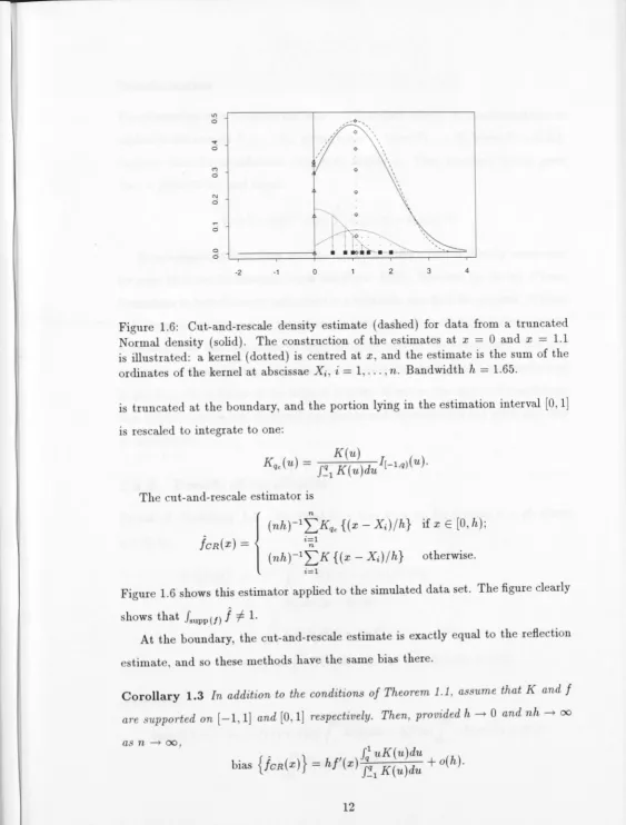
Figure 1.6: Cut-and-rescale density estimate ( dashed) for data from a truncated

Normal density (solid). The construction of the estimates at x = 0 and x = 1.1 is illustrated: a kernel (dotted) is centred at x, and the estimate is the sum of the

ordinates of the kernel at abscissae Xi, i = 1, ... , n. Bandwidth h = 1.65.

is truncated at the boundary, and the portion lying in the estimation interval

[O

,

1]

is rescaled to integrate to one:

The cut-and-rescale estimator is

if x E [0, h);

otherwise.

Figure 1.6 shows this estimator applied to the simulated data set. The figure clearly

shows that fsupp (/)

J

-f 1.

At the boundary, the cut-and-rescale estimate is exactly equal to the reflection

estimate, and so these methods have the same bias there.

Corollary 1.3 In addition to the conditions of Theorem 1.1, assume that K and

J

are supported on

[-1

,

l]

and [O

1]

respectively. Then, provided h --t O and nh--+ oo

as n --+ oo,

{

.

}

J.1

uK(u)du bias fcR(x)

=

hf'(x) ;~

1

K(u)du

+

o(h).

[image:24.609.30.594.9.751.2]

(25)

Transformation

Transformation may be useful for removing boundary effects. A transformation tis applied to the sample

Xi,

...

,

Xn

,

giving a new data set

Yi

,

...

,

Yn

where

1-':

=

t(Xi)-Suppose that the transformed data have density g. Then standard theory gives

f

(x)

=

g(t(x))t'(x)

,

and hence

n

JT(x)

=

(nht

1

t'(x)

L

K

[

{t(

x)

- t(Xi)}/h].

i=l

Transformations have been used to reduce boundary bias in density estimation

for some time, see for example Copas and Fryer (1980). However, the theory of tran-formations in kernel density estimation is a relatively new field for research. Marron and Ruppert (1994) propose transforming from a density with bounded support to a density with first derivative of approximately zero at the boundaries. The new density is estimated using reflection for boundary correction, and backtransformed to produce the estimate of the original density. However, the choice of transforma-tion involves estimation of several parameters and the method is not quick and easy

to implement.

1.3.2 Proofs of corollaries

Proof of Corollary 1.1 Provided h -+ 0 as n -+ oo, for a point x

=

qh where

q E

[O,

1),

E

{f(x)}

h-1

l

r

o

x+h

K{(x

-y)/h

}f

(y)dy

[q

1

K(u)f(x

-

hu)du

1-qi K(u){f(x)

-

huj'(x)

+

· · ·

}

du

f(

x)

[

q

1

K(u)du

-

hj'(x)

[

q

1

uK(u)du

+

o(h).

Therefore,

bias {

f

(x)}

-

f(

x)

+

f(

x)

1-

qi

K(u)du - hj'(x)

1-

qi uK(u)du

+

o(h)

-

f

(x)

1

K(u)du

+

O(h)

.

(26)

•

Proof of Corollary 1.2 Provided h - t O as n - t oo, for a point x

=

qh where

q E

[O

,

1),

E {

j

R ( X)}

=

1i-1 ( E [ K { ( X - Y) / h}]

+

E [ K { ( X

+

Y) / h}] )

Therefore,

=

h-1

[la

x+

h

K{(x -y)/h}f(y)dy

+

1-

x+h

K{(x

+

y)/h}f(y)dy]

=

1-

q

1

K(u)f(x - hu)du

+

1 :_

1

K(2q - u)f(x - hu)du

=

f(x)

{1-q

1 K(u)du

+

1:_

1 K(2q - u)du}

-hf'(x)

{1-

q

1 uK(u)du

+

1 :_

1 uK(2q - u)du}

+

o(h)

=

f(x)

{1-q

1 K(u)du

+

i

1

K(u)du}

-hf'(x)

{1-q

1 uK(u)du

+

i

1

(2q - u)K(u)du}

+

o(h).

bias {JR(x)}

=

2hf'(x) i\u - q)K(u)du

+

o(h).

•

Proof of Corollary 1.3 Provided h - t O as n - t oo, for a point x

=

qh where

q E

[O,

1),

E {JcR(x)}

=

h-1

Jo

rx

+h

KcR{(x - y)/h} f(y)dy

J~

1 K(u)f(x - hu)du

=

_J~

1 K(u)du

, J~

1 uK(u)du (h)

=

f(x) - hf (x) f~1 K(u)du

+

o .

Therefore,

• }

Jq

1

uK(u)du

bias {fcR(x)

=

hf'(x) f~i K(u)du

+

o(h).

•

(27)

1.4 Intensity function estimation

1.4.1 Poisson processes

A Poisson process is a mathematical model describing the location of point events occurring completely at random in JRd, for example, the times of emissions from

a radioactive source or the location of raisins in a cake. The basic theory and

properties are well known, see for example Feller (1968).

The three characteristic features of a homogeneous Poisson process on [0, oo)

with rate or intensity parameter A are:

1. The number of points in each finite interval [ui, vi) has a Poisson distribution

with mean A(vi - ui)

-2. The numbers of points in disjoint intervals are independent random variables.

3. The distributions are stationary: they depend only on the lengths of the

in-tervals.

An important property of the homogeneous Poisson process is that conditional on the number of events N in the interval of interest, say [0, T) the times of the events are independently uniformly distributed over [0, T).

A Poisson process can be generated from sums of independent exponential ran

-dom variables: suppose that { Z1, Z2, ... } are independent exponential random va

ri-ables with parameter A and mean 1/ A. Let Y;

=

I:

~=

l

Zi · Then

{Yi

,

Y;, ... } is a

Poisson process with parameter A. Note that Y; ,.._, Gamma (A, i) with density

y

>

0,

so that E(Y;)

=

i/A and var(Y;)

=

i/A2•

Random events need not occur uniformly in JRd: events may occur randomly with some locations being more likely than others, for example the locations of burglaries in a city, or the times of arrivals at a university cafeteria.

A non-homogeneous Poisson processes on [0, oo) is determined by a rate or in-tensity function A(

t)

2:

0. The process is defined by the following properties:

(28)

1. The number of points in each interval ( Ui

vi]

has a Poisson distribution with

mean J;: >.(t)dt.

2. The numbers of points in disjoint intervals are independent random variables.

A non-homogeneous Poisson process can be simply related to a homogeneous

Poisson process: if

{Yi

,

Y;, ... } is a Poisson process with unit mean, then writing

A(t)

=

J~>.(x)dx and Xi= A-

1(1':)

,

{X1

,

X2

,

---}

is a non-homogeneous Poisson

process with intensity function >.(t).

For the non-homogeneous Poisson process, conditional on N, the times of the

events are independently distributed over [O T) with density >.(t)/ A(T). Thus >.(t)

can be considered as a density of sorts with the difference that A(T)

=

J{

>.( t) dt is unlikely to equal 1.

There are a number of ways of simulating a realisation of a non-homogeneous Poisson process on [O, 1], see for example Devroye (1986). A simple (but not always very efficient) method, based on the analogy between intensities and densities, is to first generate a Poisson random variable N with mean A(l), and then to generate {Xi} as the order statistics of a sample of size N from the distribution with density

>.(t)/ A(l). Another method uses inversion of the integrated rate function and the

exponential spacings characteristic.

In our simulations in Chapter 3, we used the thinning method, which is similar to the rejection method of generating points from a specified density. In the thinning

method, points are generated from a Poisson process on [O, 1] with rate µ where

µ ~

>.(t).

A prospective event occurring at time t E [O, 1] is accepted with probability

>.(t)/

µ. The "thinned" process, consisting of the accepted events, is a realisation of

the non-homogeneous process with intensity >.(t).

1.4.2 Kernel estimator of intensity function

Leadbetter and Wold (1983) point out that a common feature of density and

inten-sity estimation is that the function to be estimated is the derivative of a function with a natural discontinuous estimator. The target estimator can therefore be

ob-tained by smoothing the steps using a differentiable function, and differentiating.

(29)

The obvious estimators of the distribution function and the integrated rate func-tion are

n N

F(x)

=

n-1

L

I(Xi

:S

x) and A(x)

=

L

!(Xi

:S

x),

i=l i=l

where N is the number of events of the Poisson process in the interval [O, T). Smooth versions of these can be obtained by replacing !(Xi

:S

x) with a differentiable function

5 {

(x -

Xi)/h}. The required estimators,

}(x)

and

X(x)

,

are therefore given by

n N

f(x)

=

(nh)-1

L5'{(x

-Xi)/h} and

X(x)

=

h-1

L5'{(

x

-

Xi)/h}.

i=l i=l

This derivation focusses on the similarity between the distribution function and the integrated rate function, and leads to another interpretation of the kernel function K - as the derivative of a smoothed indicator function. The kernel estimator of

the intensity function is

N

~(x)

=

h-1

L

_K

{(x - Xi)/h}.

i=l

We shall derive the distribution of this estimator in Chapter 3, and therefore delay

discussion of its bias and variance until then.

1.5 Bootstrap confidence bands for kernel curve

estimates

In a non-parametric setting, the bootstrap is a Monte Carlo based method of obtain-ing properties of the distribution of a particular statistic without making assump -tions about its distributional form. Much of the recent research into the bootstrap is aimed at finding reliable, automatic, data-based methods of calculating confidence intervals, but bootstrap methods can also be used to determine other measures of

statistical ac~uac y such as bias and prediction error.

Traditional confidence intervals for a parameter 0 are often based on the distri-bution of the asymptotically pivotal statistic T

=

(0 -

0)/'r(B), where -r(B) is an appropriate sample-based scale estimate, or on the non-pivotal statistic S

=

0 - 0.

(30)

I

I•

Bootstrap confidence intervals based on T, known as percentile-t intervals, can be

shown to be more accurate than intervals based on S, known as percentile intervals; see Beran (1987) and Hall (1992a). We shall derive below the symmetric percentile-t

bootstrap confidence interval for a single parameter 0, but shall first introduce some

necessary concepts and notation.

We regard the parameter 0 as a functional of the population distribution func -tion F, and denote it 0(F). The bootstrap estimate of 0(F) is the same functional

of the empirical distribution function

F:

8

= 0(F). For example, the bootstrap est i-mate of the population meanµ=

J

xdF(x) is the sample mean

X

=

J

xdF(x). Let X* = (X;, ... , X~) be a resample drawn from the original sample X = (X1 , . . . , Xn), let

ff

·

be the empirical distribution function of the resample, and let

e·

= 0(

fe

·)

be the same functional of the bootstrap resample. Then T*, the bootstrap estimate

of T, is obtained by replacing

8

by B* and 0 by

8

in the expression for T, so that

T* = (B* -8)/T(B*). The bootstrap 'works" because by judicious choice of the sa m-pling mechanism, the distribution of T* conditional on X , known as the bootstrap distribution of T*, is the same as that of T.

A symmetric

a%

confidence interval for T is given by (-t, t), where P(-t ~

T ~ t) = a. Without making assumptions about the distribution of T we estimate

the quantile t by the bootstrap as follows. A number, B, of resamples are drawn from X , T* is calculated for each resample, and our estimate

i

of t is the a-level quantile of the empirical distribution of IT*I. The symmetric percentile-t bootstrap

confidence interval for 0 is then simply

(8 -

if

,

8 +if).

In conventional problems with a fixed number of parameters and unknown

distri-bution function F, bootstrap confidence intervals for 0 are more accurate than tra-ditional Normal approximation intervals. The reason, which is revealed by an Edge -worth expansion argument (see for example Singh (1981), and Hall (1988, 1992a)), is that the bootstrap correctly estimates first order departures from normality which are due to skewness, whereas traditional Normal theory does not. The essence of the

argument (see Hall (1992a, p83)) goes as follows: the pivotal statistic Tis generally

(31)

asymptotically Normal, and so its distribution function can be expanded as

G

(x)

=

P(T

s;

x)

=

cp

(x)

+

n-

1

_l

2

_q(x)</>(x)

+

_O(n-

1₎_,

{1.6)

where q is an even quadratic polynomial and~,</> are respectively the standard Nor-mal distribution and density functions. The bootstrap estimate of G can similarly be expanded as

where the polynomial

q

is obtained from q by replacing unknowns such as skewness by their bootstrap estimates. Since

q

-

q

=

Op(n-1₁2_),

that is, the bootstrap approximation to G is in error by only n-1. This is an improvement over the usual Normal approximation, G ~ ~, which is in error by n-1

/2 as shown in {1.6).

In kernel curve estimation, only the data points within a neighbourhood of width h of x contribute to the estimate at x, and so the effective sample size is nh rather than n. The smaller effective sample size leads to a worsening of the convergence rate, but bootstrap methods still perform better than Gaussian theory methods, as we shall see below.

The effective sample size of nh can be interpreted as meaning that our procedure is equivalent to estimating h-1

":: n115 parameters, a number which increases with

n. Thus curve estimation problems are sometimes referred to as infinite (number of) parameter problems.

A confidence band for a curve ,( x) on an interval I is the region between two curves,

LB(

x)

and

UB(x)

,

x

E I , where

LB(x)

and

UB(x)

are chosen to ensure that th true curve is covered by the band

[LB(x)

,

UB(x)]

with probability o:; that

1s,

P{LB(x)

s;

,(x)

s;

UB(x) for all

x

EI}= o:.

When d termining a confidence band on I or a simultaneous confidence interval for a finite s t of points in I , rather than a confidence interval for a single point, our

(32)

interest moves from Tor ITI to supz

T(x)

or supz IT(x)I. The asymptotically pivotal statistic

T(x)

=

{i(x) -

,(x)}/T{'Y(x)}

is a stochastic process in

x

which can be

shown to converge to a stationary Gaussian process U(x) with known covariance

structure.

Confidence bands can be constructed based on the distribution of supz U(x).

Extreme value theory for Gaussian processes has been well studied; see for example

Hall (1979), Leadbetter et al (1983). The extreme value method of constructing

con-fidence bands for kernel curve estimates was first proposed in Bickel and Rosenblatt

(1973) for kernel density estimates. However, the convergence of U(x) to supz U(x)

is so slow, typically (log

nt

1

, see Hall (1991), that extreme value confidence bands

are of no use in practice, being much too wide, unless the sample size is simply

enormous.

The bootstrap, then, is an especially useful tool for the construction of confidence

limits or bands for kernel curve estimates, allowing us to empirically estimate the

distribution of supzT(x). The convergence of the bootstrap approximation to the

distribution of supz

T(x)

can be shown to be much faster than (log

n)-1;

for example, Hall (1991) derives the rate of (nht1_l2_{(log n)}2 _in_{the case of}_{the kernel}_density

estimator. In Chapter 3, we derive a similar comparison for the kernel intensity

estimator.

In the case of non-parametric curve estimation, the algorithm described above

produces a confidence interval for E

1'

rather than for I itself. Recall that the

bootstrap approximates the distribution of (1 - 1

)/T(7)

by that of (i* - 1)/T(i*).

However, as

1'

is a "linear" function of the data in the sense that ')'

=

~?=

1 f(Xi)

for some function f, 7*

=

~f=

1 f(Xt) has the property that E (i*IX)

=

1',

so that

bias (i*IX)

=

0. Note that

1' -

1

=

1' -

E7

+

bias (7). Then in estimating the distribution of

1' -

₁ by that of 7* -

1',

we are estimating bias (1) by bias (i*).

But bias (1'*)

= O

so that we are effectively setting bias (1) to zero and estimating

(1- E7)/T(7) not (1-1)/T(7).

In the remainder of this thesis, we will explicitly recognise that the bootstrap

algorithm produces confidence intervals for E

1'

by expressing statistics such as

T

and

T*

in the form

T(x)

=

{'Y(x)

-

E7(x)}

/

T{7(x)}

and

T(x)*

=

{'Y(x)*

(33)

Ei*(x)}

/

T{i*(x

)}

. Confidence

intervals for

Ei can be correc

ted for bias to obtain

the required confidence intervals for _{1 .}

The simplest method of bias correction is to undersmooth

i

to such an extent

that its bias becomes negligible. Our confidence interval can then be regarded as one

for I as well as for E

i-

We will use this approach in Chapter 3. Another frequently

used method is to explicitly correct the confidence interval for bias using an estimate

of the asymptotic bias (for example

(-lY

~"'hr j(rl(x) in the case of density

estima-tion). Bootstrap iteration could also potentially be used to increase the accuracy of

the bootstrap estimate in this context; see for example Hall (1992a). However, it is

possible that adding another level of bootstrap sampling and calculation of coverage

probabilities would increase the computing time above practical limits in the case

of confidence bands.

This completes our general overview of the bootstrap but we will now add some

more specific details. In general, the bootstrap resamples X* are drawn from X,

and the bootstrap estimate of

O(F)

is

O(F)

,

where Fis the empirical distribution

function. However, it has also been proposed to smooth the sample empirical

dis-tribution function and resample from that, thereby avoiding repeated values in the

resample X*; see for example Silverman and Young (1987). Although Silverman and

Young show that in some cases the smoothed bootstrap does improve performance,

Hall et al (1989) show that smoothing is really only beneficial when the quantities

under study depend in some way on local properties of the underlying distribution

F. The unknown factor in this is how much to smooth. Hall (1992a) suggests

that we should not smooth too much; oversmoothing causes a sharp deterioration in

performance. In Chapter 3, we use both the smoothed bootstrap and conventional

bootstrap resampling.

1.6 Motivation and summary of thesis

In industrial settings, observations may be collected in the form of point events

occurring randomly in space or time; such events might be for example the time

of accidents, the failure times of machines, or the location of point faults along a

(34)

'

8

"' VJ C: _Q) ₀

> _~

Q)

0 ~

8

E

::, C:

Q)

-_i;j~

3 0

E _"'

::, (.)

0

0 10000 20000 30000 40000 t (days)

Figure 1.7: Cumulative number of coal mining disasters: 1851-1962

railway track. The analysis of industrial accidents usually aims to determine possible trends in the rate of occurrence of these events: an increase in the occurrence rate would lead to action to introduce new preventative measures. Similarly the analysis of failure times of industrial equipment concentrates on trends in the failure rate. In both cases, the main interest may be in either the global trend of a series of data or in early detection of an undesirable trend in the most recent data.

In this thesis we shall analyse the intensity of coal mining disasters using the classic data set given by Jarrett (1979) and previously studied by (among others) Maguire et al (1952), Barnard (1953), Cox and Lewis (1966) and Boneva et al (1970).

The data set gives the time interval in days between 190 successive severe explosions in mines for the period 15 March 1851 to 22 March 1962. The cumulative number of disasters is plotted against tin Figure 1.7.

A major issue in previous analysis of these data has been the detection of trends in the accident rate. For example, both Barnard (1953) and Cox and Lewis (1966) fit exponential models to the intensity function, thereby showing that it is decreasing. However, in our view, kernel estimation of this intensity, as used in Diggle (1985),

Diggle and Marron (1988) and this thesis, is a more flexible tool for preliminary analysis as it shows not only the general decreasing trend, but also reveals peaks at about 8,000 days and 32,000 days (see Figure 2.6, panels C and D, on page 44).

[image:34.607.16.595.20.757.2]

(35)

In Chapter 3, we develop methods for calculating confidence bands for the

in-tensity function of an inhomogeneous Poisson process, and apply them to the coal

mining disaster data. Using this confidence band, we can not only address the

same issue of global trend as is answered by parametric analysis, but also determine

whether the additional information about the data revealed by the non-parametric

analysis, the apparent peaks, is likely to be real or merely a chimera of the

non-parametric methodology.

It is especially important in the case of intensity estimation to adequately adjust

for edge effects because the process continues unobserved outside the observation

interval and more data might become available at any time. The boundary bias

would ideally be no larger than the bias in the interior so that if more recent data

became available, the estimate based on the smaller old data set would co-incide

with that based on the new enlarged data set. We also note that if early detection

of undesirable trends in the most recent data is the main purpose of the analysis, it

is essential that the boundary bias be properly adjusted.

In Section 1.3, we described the traditional boundary kernel, reflection and cu

t-and-rescale methods of reducing boundary bias. Clearly the boundary kernel method

is the most effective, reducing the boundary bias from 0(1) to 0(hr), the size of

the interior bias, whereas the reflection and cut-and-rescale methods reduce the

boundary bias to only 0( h).

However, the speed and ease of application of an estimator are very important

considerations for the applied statistician-complex methods tend not to be used if

there are simple methods that are nearly as good. The boundary kernel estimator

shares a major drawback with the cut-and-rescale estimator, namely, its

implemen-tation is complicated in that a different kernel is constructed at each estimation point

in the boundary region. In addition, the computation of that kernel requires solving

a system of equations. On the other hand, the reflection estimator is extremely

sim-ple to apply: the same kernel is used throughout the estimation interval and that

kernel is simple to implement. Clearly then, there is a place for a new estimator

which combines the best features of the boundary kernel and reflection estimators:

boundary bias of order 0( hr) and applicability over the whole stimation interval.

23

Some problems in kernel curve estimation

I