Evaluating uncertainty in convective cloud microphysics using statistical emulation

RESEARCH ARTICLE

10.1002/2014MS000383

Evaluating uncertainty in convective cloud microphysics using

statistical emulation

J. S. Johnson1_{, Z. Cui}1_{, L. A. Lee}1_{, J. P. Gosling}2_{, A. M. Blyth}1,3_{, and K. S. Carslaw}1

1_{Institute for Climate and Atmospheric Science, School of Earth and Environment, University of Leeds, Leeds, UK,}2_School

of Mathematics, University of Leeds, Leeds, UK,3National Centre for Atmospheric Science, University of Leeds, Leeds, UK

Abstract

the amount and intensity of precipitation as well as dynamical features. Realistic simulation of these cloud properties presents a major challenge. In particular, because models are complex and slow to run, we have little understanding of how the considerable uncertainties in parameterized processes feed through to uncertainty in the cloud responses. Here we use statistical emulation to enable a Monte Carlo sampling of a convective cloud model to quantify the sensitivity of 12 cloud properties to aerosol concentrations and nine model parameters representing the main microphysical processes. We examine the response of liquid and ice-phase hydrometeor concentrations, precipitation, and cloud dynamics for a deep convective cloud in a continental environment. Across all cloud responses, the concentration of the Aitken and accumulation aerosol modes and the collection efficiency of droplets by graupel particles have the most influence on the uncertainty. However, except at very high aerosol concentrations, uncertainties in precipitation intensity and amount are affected more by interactions between drops and graupel than by large variations in aero-sol. The uncertainties in ice crystal mass and number are controlled primarily by the shape of the crystals, ice nucleation rates, and aerosol concentrations. Overall, although aerosol particle concentrations are an important factor in deep convective clouds, uncertainties in several processes significantly affect the reliabil-ity of complex microphysical models. The results suggest that our understanding of aerosol-cloud interac-tion could be greatly advanced by extending the emulator approach to models of cloud systems.

1. Introduction

The interaction of aerosols with clouds is the largest uncertainty in the quantification of Earth’s changing energy budget over the industrial period [Boucher et al., 2013]. To assess the climate impact of aerosol-cloud interaction, global model simulations of aerosol-clouds and aerosols are needed, which presents substantial problems in terms of resolving the key processes in low resolution and computationally demanding climate models. However, even dedicated cloud-resolving models that include detailed aerosol and cloud micro-physical processes are still subject to large uncertainty. Microphysics in clouds is complex and includes at least the activation of aerosol particles to form drops, ice formation, diffusional growth of cloud particles, and interactions between multiple types of cloud particles. The spatial scales of cloud microphysics span several orders of magnitude, and microphysical processes are interactive and can affect cloud dynamics and thermodynamics. Many cloud microphysical processes are not explicitly represented in models and therefore must be parameterized. Parameterizations of processes are based on observations, laboratory experiments and theoretical studies. However, such parameterizations are constrained by either limited observations, idealized conditions in the laboratory or theoretical assumptions, and, hence, cloud model outputs are subject to parametric uncertainty. It is important to understand the uncertainty to improve the performance of microphysical schemes for better weather forecasts and climate projection.

One approach for understanding model uncertainty is to compare different microphysics schemes within the same host dynamics model.Morrison and Grabowski[2007] showed that a one moment bulk scheme may produce significant errors relative to the bin model for some cases. For bulk parameterizations, a higher moment scheme generally produces better simulations [Milbrandt and Yau, 2006;Morrison et al., 2009].

McCumber et al. [1991] swapped parameters between a 3-class and a 2-class ice scheme and showed that the 3-class scheme is better than the 2-class scheme. Nevertheless, the most popular method is to test a sin-gle parameter or a small number of parameters in the same microphysics scheme through a one-at-a-time (OAT) test approach. The OAT test evaluates the change in the model output from some baseline case with Key Points:

Processes driving uncertainty in convective cloud physics are identified

Emulation makes comprehensive sensitivity analysis of cloud models feasible

Aerosol effects can be smaller than many microphysical uncertainties

Correspondence to: J. S. Johnson, [email protected]

Citation:

Johnson, J. S., Z. Cui, L. A. Lee, J. P. Gosling, A. M. Blyth, and K. S. Carslaw (2015), Evaluating uncertainty in convective cloud microphysics using statistical emulation,J. Adv. Model.

Earth Syst.,7, 162–187, doi:10.1002/

2014MS000383.

Received 2 SEP 2014 Accepted 6 JAN 2015

Accepted article online 13 JAN 2015 Published online 11 FEB 2015

This is an open access article under the terms of the Creative Commons Attri-bution License, which permits use, dis-tribution and reproduction in any medium, provided the original work is properly cited.

respect to a perturbation in a single model input. For example,Gilmore et al. [2004] tested various intercept parameters from an assumed size distribution conjointly with two particle densities for hail/graupel. They found that the accumulated precipitation was very sensitive to the changes in the parameters.Adams-Selin et al. [2013] showed the sensitivity of cloud properties to different graupel size distributions as well as the complete removal of graupel.Dearden et al. [2011] applied a factorial method to a single column model to investigate the sensitivity of each one in a suite of microphysics schemes.Guo et al. [2014] adopted a quasi-Monte Carlo sampling approach and a generalized linear model to analyze the sensitivity of properties of stratocumulus and shallow cumulus clouds to model parameters. With the intention of investigating the interactions between the parameters,Posselt and Vukicevic[2010] developed a Markov chain Monte Carlo algorithm to identify the uncertainty in simulating deep convective cloud with a one-dimensional model. They mapped the joint probability density function of parameters and model output state variables and found that a complex relationship exists between parameters and model output. However, thePosselt and Vukicevic[2010] algorithm requires 106_{simulations in order to obtain the stationary joint probability density} function for a 10 parameter analysis.

Although these previous model investigations have highlighted interesting features and dependencies as to how cloud responses change with respect to individual model parameters, very few highlight where uncertain input parameters interact and nearly all leave much of the defined parameter uncertainty space unexplored. Often this is due to the extremely large computational burden that results from the need to run the model simulator many times in order to explore the joint effects of uncertain input parameters through simultaneous parameter perturbations. With multiple uncertain inputs this can easily become impractical.

In this study, we explore the parametric uncertainty in a model of a single convective cloud, applying statistical algorithms that enable us to explore both the model sensitivity to uncertainty in individual param-eters and the model sensitivity to parameter interactions at a relatively low computational cost. We balance the physical representation of the microphysical processes and the computational demand by simulating a single meteorological environment, but with bin-resolved microphysics. The simulation of a single cloud cannot account for the complex interaction between the dynamics and the microphysics that can occur in all conceivable meteorological environments. However, as we show, a detailed analysis of parametric uncertainty in cloud microphysics enables the most important parameters to be identified, which in future would allow a reduced parameter set to be applied to an ensemble of clouds formed in a range of environments.

Our approach is to use statistical emulation [O’Hagan, 2006] and variance-based sensitivity analysis [Saltelli et al., 2000], covering the full parameter space defined by the input parameter uncertainties in the calcula-tion of our sensitivity measures. This is made possible by following the structured Bayesian statistical approach used byLee et al. [2011, 2013], who examine the effects of parametric uncertainty on the simu-lated cloud condensation nuclei concentration within a global aerosol model. This approach takes advant-age of statistical methodologies including expert elicitation [O’Hagan et al., 2006], statistical experiment design [Santner et al., 2003], Gaussian process emulation [O’Hagan, 2006;Rasmussen and Williams, 2006], and probabilistic sensitivity analysis [Oakley and O’Hagan, 2004;Saltelli et al., 2000]. The construction of a statistical emulator to represent the relationship between the set of uncertain model input parameters and the model output of interest means that we can evaluate this relationship over the full parameter uncer-tainty space for a very low computational cost. Therefore, this enables us to evaluate the sensitivity of the output to all of the uncertain inputs simultaneously, which allows for interaction effects to also be considered.

These methods allow us to determine how this uncertainty propagates through the model and affects the cloud responses.

The paper is structured as follows. In section 2, we describe MAC3 and the uncertain parameters, micro-physical processes, and cloud responses that we wish to explore through our simulations for the formation of a deep convective cloud. In section 3, we outline the Bayesian statistical methods that we use to evaluate the sensitivity of the cloud responses to the defined parametric uncertainty. In section 4, we present the results of the sensitivity analysis, and our findings are summarized and discussed in section 5.

2. The Model of Aerosols and Chemistry in Convective Clouds, MAC3

2.1. Model Description

MAC3 is a complex cloud microphysics model that simulates the formation and development of convective clouds, given an initial set of aerosol and atmospheric conditions. MAC3 was originally developed through the work ofReisin et al. [1996], and has been extended and further developed byYin et al. [2005]. Within the model, the cloud and aerosol microphysics are size-bin resolved. Hydrometeors (drop, ice crystal, grau-pel, and snow) are resolved with 34 size bins from 3 to 6400lm for drops and 3 to 8540lm for ice particles. Aerosol particles are resolved in 43 bins. The warm microphysical processes represented in the model include activation of CCN, diffusional growth, collision-coalescence, breakup, and evaporation. The repre-sented cold processes are immersion freezing, deposition freezing, contact freezing, secondary ice produc-tion by the Hallett-Mossop mechanism, diffusional growth, and interacproduc-tion between hydrometeors. The model is run in axisymmetric coordinates and the bin schemes are based on the method of moments by

Tzivion et al. [1987]. MAC3 has been used to simulate and evaluate a variety of convective clouds and cloud properties, such as warm rain in shallow cumulus [Blyth et al., 2013], secondary ice production [Huang et al., 2008], aerosol effect [Cui and Carslaw, 2006;Cui et al., 2006], aerosol-cloud-precipitation interaction [Cui et al., 2011a], and the coupled effect of aerosol and moisture [Cui et al., 2011b].

The cloud simulated in this paper is a deep convective cloud in a continental environment, which has been extensively studied [e.g.,Hobbs et al., 1985;Respondek et al., 1995;Yin et al., 2005].Yin et al. [2005] compared the simulated cloud properties with observations. They found that the model reproduced the cloud reason-ably well, including the base height, size of the main updraught core, updraught speed at cloud base, start time of the updraught decay, location and time of the maximum liquid-water content, concentration of droplets, first appearance of graupel, and location of the first radar echo. The initial conditions used for the thermodynamical variables here are the same as inYin et al. [2005].

2.2. Choice of Uncertain Input Parameters

Eleven input parametersX5fX1;X2;…;X11gwere selected to represent the main processes acting in the simulation of the deep convective cloud. A short description of each input parameter is given below, along with our assessment of the uncertainty in the values they may take, which we specify as a range of plausible values on either an absolute or a multiplicative scale. These uncertainty assessments were obtained via a small expert elicitation exercise in which information from the current literature was combined with exper-tise and knowledge of the capabilities of the MAC3 model itself. The inputs and uncertainty specifications are also summarized in Table 1.

The term ‘‘parameter’’ refers to any model quantity that can be independently perturbed to affect model output and will be used as an input to our statistical model. Some of our chosen parameters are physical quantities that can be measured in nature, such as particle density. Other parameters refer to model quanti-ties that have no direct analogue in nature; they are model artifacts that are necessary because of model simplification. We also include aerosol particle concentrations as a parameter, even though this quantity might be considered a boundary condition on the model.

2.2.1. Graupel Density (X1)

Morrison[2013] treated the graupel density as a variable rather than a constant term and so used a range of graupel densities. In this study, we vary the graupel density over the range used inMilbrandt and Morrison

[2013] of (0.05, 0.85) g cm23.

2.2.2. Threshold Between Ice Crystal and Graupel (X2)

This is a threshold value at which drops with radii larger than a given size (default 100lm) are transferred to graupel upon freezing; otherwise, they are considered as ice crystals [Reisin et al., 1996]. The uncertainty range for this threshold is set to be from 50 to 800lm.

The threshold method used in this model and others imposes a fundamental problem because it necessi-tates artificial conversion processes. The latest scheme ofMorrison and Milbrandt[2015] overcomes this issue by predicting particle properties and avoiding the unphysical constrained thresholds for conversion between predefined ice-phase classes.

2.2.3. Immersion Freezing (X3)

Immersion freezing occurs when an ice nucleus is immersed within a liquid drop. Whether a drop freezes or not depends on supercooling, as well as the size, surface property, and chemical composition of the immersed nucleus. Two hypotheses have been proposed. One is stochastic and the other singular [Murray et al., 2012]. However, the widely used Bigg scheme for immersion freezing, also used in this paper, does not take account of the chemical composition of ice nuclei. The ice nucleating efficiency of particles varies across several orders of magnitude [Diehl and Wurzler, 2004]. To account for this variation in our simulations, the parameter A in the Bigg scheme [seeCui et al., 2006, equation (5)] is multiplied by a factor between 0.01 and 100.

2.2.4. Deposition Freezing (X4)

Deposition freezing refers to the formation of ice in a supersaturated vapor environment, and condensation freezing is the sequence of events whereby a cloud condensation nuclei (CCN) initiates freezing of the con-densate [Vali, 1985]. In cloud modeling, it is practically difficult to distinguish between these two freezing modes. MAC3 uses theMeyers et al. [1992] scheme for deposition freezing, which predicts the number con-centration of ice crystals due to deposition-condensation freezing as a function of supersaturation with respect to ice. TheMeyers et al. [1992] scheme was originally applied over the temperature range from 27_{C to220C, from 2 to 25% ice supersaturation, and from25% to 4.5% water supersaturation. InMeyers}

et al. [1992], the number of ice crystals is predicted via the equation:

Nid5expða1bSiÞ;

whereSiis the supersaturation with respect to ice, and the constantsaandbare the intercept and slope

parameters for this relationship, respectively, which are derived from measurement. In our simulations, the parameterbhere is multiplied by a factor between 0.05 and 2.

2.2.5. Terminal Fall Speed for Ice Crystal (X5)

The terminal fall speed of a cloud particle is the steady velocity achieved when the drag force balances the gravitational force. There is little uncertainty about the terminal fall speeds of liquid drops. However, the uncertainty in terminal fall speeds of ice particles is large. This uncertainty could originate from the relation-ship between the size and mass of an ice particle because of the irregular shape. Alternatively, it may also come from the drag force since the theory available for calculating drag force is restricted to semiempirical

Table 1.The Uncertain Model Parameters

Parameter Uncertainty Range Effect

X1 Graupel density 0.05–0.85 Absolute

X2 Threshold between ice crystal and graupel 50–800 Absolute

X3 Immersion freezing coefficient 0.01–100 Scaled

X4 Deposition freezing coefficient 0.05–2 Scaled

X5 Terminal fall speed for ice crystal 0.2–4 Scaled

X6 Graupel aerodynamic parameter 0.5–2 Scaled

X7 Collection efficiency of drops by graupel 0.01–10 Scaled

X8 Collection efficiency of ice crystals by graupel 0.1–3 Scaled

X9 Capacitance of ice crystals 0.01–10 Scaled

X10 Aitken and accumulation modes of aerosol 0.01–4 Scaled

methods, and the drag coefficient is extremely difficult to determine accurately [Pruppacher and Klett, 1997]. Fall speed differences between different schemes can be very large [Mitchell and Heymsfield, 2005]. The terminal fall speeds (in cm s21_{) for ice particles in MAC3 are obtained by theB€ohm[1989] formulation} which is a function of the particle mass, the kinematic viscosity, the Reynolds number, and the ratio of the effective projected area to the circumscribed area of the particle. The terminal fall speed for ice crystal is multiplied by a factor between 0.2 and 4.

2.2.6. Graupel Aerodynamic Parameter Affecting Terminal Fall Speed (X6)

The terminal fall speed of graupel is calculated according to theB€ohm[1989] formulation:

Vg5

Reg

2q_a p A

1=2

;

where Re is the Reynolds number,gis the kinematic viscosity,qais the air density, andAis the

circum-scribed area defined as the area of the smallest circle or ellipse that completely contains the effective pro-jected area. The Reynolds number is related to the Best number throughX5CDRe, whereCDis the drag

coefficient. There are therefore several sources of uncertainty in the terminal fall speed: the graupel density, the effective projected cross-sectional area, the circumscribed area, and the relationship between the Reyn-olds number and the Best number.Heymsfield and Wright[2014] showed that the roughness can cause large differences in values of the Reynolds number for any given Best number across the whole domain, regardless of the graupel size. The Reynolds number for graupel due to its relationship with the Best num-ber is multiplied by a factor between 0.5 and 2 in our study. For simplicity, this parameter is referred to as the graupel aerodynamic parameter in the following text. Although both the graupel density (X1) and the aerodynamic parameter (X6) affect the terminal fall speed, the values of these two parameters are not correlated.

2.2.7. Collection Efficiency of Drops by Graupel (X7) and of Ice Crystals by Graupel (X8)

Factors such as the size and shape of graupel, the relative collision velocity and drop sizes can all affect the collection efficiency [von Blohn et al., 2009]. Furthermore, the graupel-drop collision kernels may signifi-cantly increase in turbulent clouds [Khain et al., 2000;Wang et al., 2005], and the degree by which the col-lection efficiency depends on temperature, humidity, and other atmospheric parameters is also unknown. The efficiency is dimensionless. In our study, the collection efficiency of drops by graupel is multiplied by a factor between 0.01 and 10, while the collection efficiency of ice crystals by graupel is multiplied by a factor between 0.1 and 3.

2.2.8. Capacitance of Ice Crystals (X9)

Ice crystals have various habits and are generally not spherical in shape. The supersaturation just above the growing surface of a nonspherical crystal is not as uniform as in the far field. The deposition/evaporation equation for crystal growth has to be modified to include the effect of crystal habit. A common method to consider the nonspherical effect is to introduce the analogy between the diffusion of heat and water vapor around a crystal to that of electrical charge dissipation from a capacitor of similar shape [Cotton et al., 2011]. In this way, theoretical capacitances for some simple shapes of crystals can be derived [McDonald, 1963]. There is uncertainty in capacitance. For example,Westbrook et al. [2008] found that the capacitance of an aggregate is close to half of the value for a sphere, whileBailey and Hallett[2012] argued that theoretical estimates of capacitance overestimate the actual growth by a factor of 2–4.Lamb and Verlinde[2011] recog-nized that it is realistic only if both the particle mass and the aspect ratio can be calculated simultaneously. The uncertainty in the capacitance parameter is set to be a factor between (0.01, 10).

2.2.9. The Concentration of the Aitken and Accumulation Modes of Aerosol (X10)

approximately 50 to 20,000 cm23, which covers more than the typical range of aerosol concentrations and is somewhat larger than used inCui et al. [2006].

2.2.10. The Concentration of the Coarse Mode of Aerosol (X11)

The measurement of coarse mode aerosol is even more variable than that of the Aitken and accumulation modes [e.g.,Reid et al., 2006]. This parameter defines the total number of coarse mode aerosol particles in the initial size distribution. The total number of aerosol particles in the coarse mode is changed by a factor between (0.01, 100) in our simulations, resulting in particle concentrations in the range 0.0045–4.5 cm23.

Together, these defined uncertainty specifications form an 11 dimensional parameter uncertainty space over which we want to evaluate outputs from the cloud microphysics model. We aim to assess how this uncertainty propagates through the model to each of a selection of model outputs in order to determine which input parameters, and hence corresponding processes and mechanisms, drive uncertainty in the cloud responses of interest.

2.3. Choice of Model Outputs

For each model run, we have simulated 80 min of cloud formation and development and recorded 12 model outputs, defined in Table 2. The selection of outputs encompasses cloud dynamical responses, cloud particle responses, and precipitation. The outputs are summary statistics taken over space and time through the centre of the cloud. It would also be possible to analyze outputs at a particular time in the cloud devel-opment, or at a specific location in the cloud. However, each cloud evolves differently depending on the parameter setting, so it is difficult to compare sensitivities without averaging in time and space.

3. Statistical Methods

In this study, we use variance-based sensitivity analysis to determine which input parameters, and therefore model processes and mechanisms, lead to parametric uncertainty in the MAC3 model outputs of interest. Evaluation of the corresponding model sensitivity measures, and so the effects of input parameter uncer-tainty on model outputs, is classically achieved using a direct Monte Carlo simulation approach. This involves running the model simulator many times over different combinations of input parameter values, but when the model is computationally expensive to run like MAC3 these calculations can quickly become unfeasible. Instead, we take advantage of the Bayesian statistical theory for building fast surrogate com-puter models, known as emulation, to construct surrogate representations of MAC3 that can be used in place of the model simulator itself to make these calculations. This structured Bayesian approach to evaluat-ing model sensitivity, originally proposed byOakley and O’Hagan[2004] and as depicted by the flow dia-gram inLee et al. [2011, Figure 1], requires us first to generate a designed set of well-spaced training runs from MAC3 over the defined parameter uncertainty space. Then, through the application of Gaussian pro-cess emulation over this training data to each MAC3 model output independently, we are able to evaluate

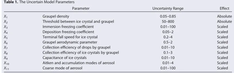
Table 2.The Output Variables Considered, with Summary Statistics for Each Output Obtained From the Simulated Uncertainty Distribu-tions Over the Full Parameter Space in Figure 5a

Model Output (Units) Min LQ Median UQ Max l r jr

lj Mean effective radius (lm) 3.62 180.37 225.09 264.60 457.15 224.10 66.34 0.30 Mean updraught speed (m s21

) 1.98 3.26 3.56 3.78 5.00 3.49 0.46 0.13

Mean downdraught speed (m s21

) 27.33 26.01 25.48 24.58 21.54 25.22 1.08 0.21 Mean value of specific drop mass (g kg21

) 0.31 0.77 0.92 1.04 1.54 0.90 0.19 0.21 Mean value of specific ice crystal mass (g kg21

) 0.04 0.35 0.51 0.73 1.65 0.56 0.27 0.48 Mean value of specific graupel mass (g kg21

) 0.01 1.02 1.35 1.64 2.73 1.27 0.54 0.42 Mean drop number concentration (cm23

) 2.15 9.77 26.70 76.19 329.51 53.13 59.99 1.13 Mean ice crystal number concentration (L21

) 0.49 39.31 94.09 205.52 3810.87 177.54 262.25 1.48 Mean graupel number concentration (L21

) 0.01 0.24 0.97 1.98 31.16 1.73 2.64 1.52 Mean reflectivity (dBZ) 14.43 47.14 51.66 58.67 67.54 51.53 8.75 0.17 Accumulated precipitation at 80 min (mm) 0.00 12.09 18.88 35.38 72.54 23.48 16.42 0.70 Maximum precipitation rate (mm h21

) 0.00 65.56 99.78 192.38 852.97 152.69 145.28 0.95

a

these model outputs across all dimensions of the parameter uncertainty space at a very low computational cost, making the variance-based sensitivity analysis of MAC3 possible.

In this section, we outline the statistical methods that come together to form this structured Bayesian approach, and we describe how each one has been applied in our analysis of MAC3.

3.1. Statistical Design for the Training Data

The aim of our sensitivity study is to determine how the defined uncertainty in each of the eleven input parameters from section 2.2 feeds through MAC3 to affect each model output of interest. Therefore, each emulator model we construct must cover the full parameter space defined by these uncertain input parameters.

Emulator training data are obtained by running a set of chosen input combinationsx5fx1;x2;…;xng,

wherexi5 xi;1;…;xi;11

, through the cloud model simulator to obtain the corresponding model outputs

y5fy1;y2;…;yng. The number of training runsnrequired to achieve a reasonable model fit for the

emula-tor is dependent on the number of active input parameters and how smoothly the simulaemula-tor output varies over the parameter space. A common practice, as discussed and supported byLoeppky et al. [2009], is to usen510druns from the model simulator for training the emulator (wheredis the number of uncertain input parameters over which the emulator is to be built), with the premise that more model runs can be added to the training data if it is found through diagnostic checks that the emulator accuracy is poor. Con-sequently, we usen5110 training runs for the MAC3 emulation here.

To achieve an optimal coverage of the parameter space with these 110 emulator training runs, we use a space filling statistical experiment design method to choose the actual input combinationsx. One of the most widely used design algorithms for this purpose is the maximin Latin hypercube [Morris and Mitchell, 1995], and this is the method we have used for our training data here. The maximin Latin hypercube

2.5 3.0 3.5 4.0

2.0

2.5

3.0

3.5

4.0

4

.5

5.0

(a)

Cloud Model: Mean Updraught (m s−1₎ Emulator Prediction: Mean Updraught (m

s

−

1)

−4 −2 0 2

−4

−2

0

2

(b)

Cloud Model: log[Mean Graupel Number Concentration (L−1_)] Emulator Prediction: log[Mean Graupel Number Concentration

(

L

−

1)

]

0 1 2 3 4

01234

(c)

Cloud Model: [Accumulated Precipitation at 80 min (mm)]1 3 Emulator Prediction: [Accumulated Precipitation at 80 min (mm)

]

1

3

0 2 4 6 8

02468

1

0

(d)

Cloud Model: [Maximum Precipitation Rate (mm hour−1_)]1 3 Emulator Prediction: [Maximum Precipitation Rate (mm hour

−

1)]

1

3

algorithm maximizes the minimum distance between points in order to ensure optimum space filling and hence a good coverage of the parameter uncertainty space.

3.2. Emulation

Emulation is a technique by which we construct a statistical representation—anemulator—of a particular aspect of a model simulator (such as the relationship between a set of uncertain inputs and an output of inter-est) that can be evaluated quickly. The approach stems from the work ofO’Hagan[1978] who described how a Gaussian process can be used to represent an unknown function. The methodology has since been further developed and applied within the literature [see e.g.,Sacks et al., 1989;Kennedy and O’Hagan, 2001;Oakley and O’Hagan, 2004;Lee et al., 2013]. In this study, we adopt the most common emulator form, using the Gaus-sian process as the basis of our emulator models. A mathematical description of GausGaus-sian process emulation is given in Appendix A, and here we describe the application of the Gaussian process emulator to MAC3.

The model outputs from MAC3 are considered independently in this work, so a separate emulator is con-structed for each model outputY. In each case, we represent the cloud model simulator as a functiongðÞof the 11 uncertain input parametersX5fX1;…;X11gover the parameter uncertainty space such thatY5gðXÞ. An emulator is then constructed to represent the input-output relationship using Bayesian statistical theory by combining the information from the model simulator in the training data with a set of prior beliefs about the behavior of MAC3. These prior beliefs are characterized in the form of a Gaussian process with a speci-fied mean and covariance structure,mðÞandVð;Þ, respectively, as detailed in Appendix A. For the 12 emu-lators here, a linear mean structure for the output with respect to all uncertain input parameters given by:

Y5mðxÞ5C1X 11

i51

b_ixi

is assumed, whereCis a constant term and thebiare unknown linear regression coefficients that are

esti-mated in the model fit, along with a Matern covariance structure forVðx;x0_{Þ. The Matern covariance} struc-ture was chosen as this form has been found to cope more easily with any slight roughnesses in the model output surface [Rasmussen and Williams, 2006], and it could easily be the case that the model output surface is not completely smooth for some of the cloud properties from MAC3.

This posterior model is the emulator, defining a fitted surface with uncertainty for the model outputYover the 11 dimensional parameter uncertainty space. We note that even though the prior mean takes a linear form here, the posterior Gaussian process is not restricted by this and can take a quite different nonlinear form, dependent on the information from the training data. The fitted surface passes through each of the training data points exactly, and given the derived mean and covariance structure, the emulator interpo-lates the outputYover the parameter space to provide an estimate ofYat all untried points along with a measure of uncertainty about this prediction.

Each emulator was fitted using the statistical software R [R Core Team, 2013], and the R package DiceKriging [Roustant et al., 2012]. In order to avoid erroneous predictions from the emulator when a model output has a natural lower bound at zero it was necessary to transform some of the cloud model outputs prior to fitting the emulator. In the results that follow, the outputs for the mean number concentrations of drops, ice crys-tals, and graupel are emulated using the natural logarithm transform given byZi5logeðYiÞ, and the outputs

for the mean ice crystal mass, the mean graupel mass, the accumulated precipitation at 80 min and the maximum precipitation rate are emulated using the cube root transform given byZi53ffiffiffiffiYi

p

. Nonetheless, in all of these cases the uncertainty and sensitivity analysis of the output variable is evaluated on the original output scale via back-transform of the emulator predictions prior to calculation of the uncertainty and sensi-tivity measures. Such transforms do have the effect of inflating the standard errors (uncertainty) about the emulator predictions on back-transformation. However, it is the mean prediction from the emulator that we take forward and use for our sensitivity analysis and we have found that this is robust to this error inflation.

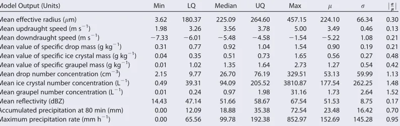
3.3. Emulator Validation

and O’Hagan[2009]. For validation, a second set of MAC3 model runs was evaluated, which we refer to as thevalidation data. This validation data contains model runs for 88 input combinations that are different to those contained in the training data. Ten of the input combinations were selected to be specifically close to training data points in the parameter space and the remainder were selected using the maximin Latin hypercube experiment design algorithm to ensure good coverage of the whole parameter uncer-tainty space in the validation. We select specific points within close proximity to the emulator training runs as well as points further away within the parameter uncertainty space as the evaluation of each of these can inform us about different aspects of the fit of the emulator. For example, points close to design runs can be highly sensitive to the hyper-parameters of the estimated correlation function within the covariance structure of the emulator model [Bastos and O’Hagan, 2009].

Figure 1 shows validation plots for a selection of the cloud responses: the mean updraught, the mean graupel particle number concentration, the accumulated precipitation at 80 min, and the maximum precipitation rate. These plots are scatterplots of the emulator mean predictions versus the actual MAC3 model output for the validation data set, with 95% confidence intervals on the emulator mean predictions calculated via the poste-rior emulator covariance structure given by equation (A3) in Appendix A. Figure 1 shows the true MAC3 model output to lie within the 95% confidence bounds of the emulator prediction for the vast majority of the valida-tion runs. Where this is not the case, the points are highlighted in red. Looking across all 12 cloud responses, the total percentage of the validation runs for which the MAC3 model output lies outside the 95% confidence bounds of the corresponding emulator prediction for any one output is no higher than 10%, and for many of the outputs this is much lower at around 5%, which we expect to be the case given we are using a 95% confi-dence bound for this diagnostic. For each model output in Figure 1, the plotted points follow reasonably close to the line of equality depicted in gray. We also see this in the corresponding validation plots for the further eight model outputs that are not shown here. This indicates that across all outputs the emulator mean predic-tion is providing a reasonable representapredic-tion of the actual model output from MAC3.

The overall uncertainty in a model outputYcan be broken down into two components: the parametric uncertainty (caused by the uncertainty in the model parameters,X) and the emulator uncertainty (the con-sequence of using the emulator rather than the model itself to evaluateY). For the emulator to be useful and capture the model signal with reasonable precision, we require the emulator uncertainty to be less than the parametric uncertainty that we are aiming to quantify. Both the emulator uncertainty and the para-metric uncertainty can be estimated through the simulation of Gaussian process functions from the emula-tor model. On comparison, we have found that the magnitude of the emulaemula-tor uncertainty ranges between 2.5% and 5.2% of the magnitude of the parametric uncertainty for the MAC3 model outputs considered in this study. This shows that in comparison to the overall parametric uncertainty in the model outputs, the uncertainty due to the emulator approximation itself is minimal.

Additional validation diagnostics to assess the model fit for each emulator have been implemented and examined, including the leave-one-out approach detailed inRougier et al. [2009], the evaluation of standar-dized model residuals and the analysis of the pivoted Cholesky variance decomposition as proposed by Bas-tos and O’Hagan[2009]. The resulting diagnostic plots from these further validations (not shown) support our conclusions here that each emulator is providing a reasonable representation of its corresponding cloud response over the parameter uncertainty space. We therefore consider each of the fitted emulator models as valid in this study, and take them forward to use in place of MAC3 for the calculation of our uncertainty and sensitivity measures.

3.4. Sensitivity Analysis

Sensitivity analysis methods provide a mechanism through which the variation in a model output can be decomposed and proportionally assigned to different contribution sources. Given an understanding of the uncertainty in a set of model input parameters, it is possible via sensitivity analysis to quantify the effect of this uncertainty on a model output of interest and determine which input uncertainties drive the variation in that output. A comprehensive overview of methods for sensitivity analysis is given bySaltelli et al. [2000].

methodology is based on the decomposition of the overall variance of an output into contributions from individual inputs and combinations of inputs together. The resulting variance decomposition is used to compute two sensitivity measures: themain effect indexand thetotal effect index, as detailed inSaltelli et al. [2000], and summarized in Appendix B. For each uncertain input parameter of MAC3, the main effect index provides a measure of the percentage by which the overall variance in the cloud model outputYcould be reduced if the input parameter was known exactly. The total effect index provides a joint measure of the individual effect of an input parameter and all interaction effects that involve that specific input. Hence, the difference between the total effect index and the main effect index gives an indication of how much an input parameter is interacting with other inputs in the cloud model. Given the complex microphysics involved in the formation of a cloud, it is possible that there may be some strong interaction effects between the uncertain input parameters for the MAC3 model outputs under investigation here.

Evaluation of the variance-based sensitivity measures for each model output from MAC3 requires many eval-uations of the output over the parameter uncertainty space. Here we use the constructed emulators in place of MAC3 and sample across the parameter uncertainty space using the extended-FAST (Fourier Amplitude Sensitivity Test) approach ofSaltelli et al. [1999] in order to compute the sensitivity measures. The extended-FAST approach to the sampling is specifically designed for sensitivity analysis, and it generates a much more efficient sample across the parameter space in comparison to the general Monte Carlo sampling approach. The calculations of the sensitivity measures for this study have been completed using the R package ‘‘sensitiv-ity’’ [Pujol et al., 2013], and the results of this sensitivity analysis are discussed in section 4.3.

4. Results

4.1. Exploratory Analysis of the Training and Validation Model Runs

To begin our analysis of how the uncertainty in the MAC3 model input parameters affects the model out-puts of interest, we explore pairwise scatterplots of the emulator training and validation model runs for all

−2.0 −1.5 −1.0 −0.5 0.0 0.5

0

5

0

100

150

200

250

300

(a)

log10(Aitken and Accumulation Modes of Aerosol)

Mean Drop Number Concentration

(

L

−

1)

−2.0 −1.5 −1.0 −0.5 0.0 0.5

2.5

3

.0

3.5

4

.0

4.5

5

.0

(b)

log10(Aitken and Accumulation Modes of Aerosol)

Mean Updraught (m

s

−

1)

−2.0 −1.5 −1.0 −0.5 0.0 0.5

−7

−6

−5

−4

−3

−2

(c)

log10(Aitken and Accumulation Modes of Aerosol)

Mean Do

wndraught (m

s

−

1)

−2.0 −1.5 −1.0 −0.5 0.0 0.5

0

1

02

03

04

05

06

07

0

(d)

log10(Aitken and Accumulation Modes of Aerosol)

Accumulated Precipitation at 80 min (mm)

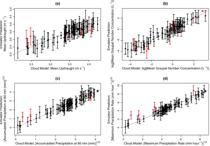
Figure 2.Pairwise scatterplots of the emulator training and validation model runs for (a) mean drop number concentration, (b) mean updraught, (c) mean downdraught, and (d) accu-mulated precipitation at 80 min (yaxis), versus the scaled Aitken and accumulation modes of aerosol concentration (xaxis). Log10(X10)50 corresponds to an Aitken and accumulation

mode aerosol concentration of approximately 5000 cm23

input/output combinations. Exam-ination of these plots has revealed that the parameter corresponding to the concentration of the Aitken and accumulation modes of aero-sol has the most influence across the cloud properties we consider. Figure 2a shows the strongest pairwise relationship that was found, between the concentration of the Aitken and accumulation mode aerosol and the mean drop number concentration. (We note here that the range of values taken by this aerosol parameter is on a multiplicative scaling, so a

log10transform is used for the plotting. The model default value from which the parameter is var-ied within this study corresponds to a value oflog10ðX10Þ50.) We see in Figure 2a that as thelog10 scaling of the aerosol concentra-tion increases, the mean drop number concentration increases exponentially. Hence, the drop number concentration increases approximately linearly with the aerosol scaling itself.

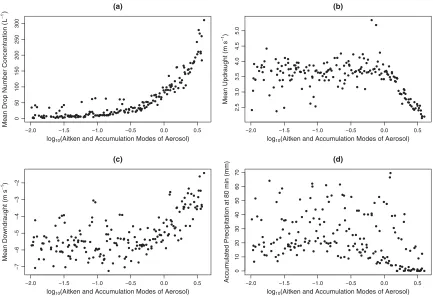
Figures 2b and 2c show the effect of the concentration of the Aitken and accumulation mode aerosol on the mean updraught and mean downdraught in the simulated cloud, respectively. These plots show that the cloud behavior changes distinctly for the higher aerosol concentrations, with these vertical veloc-ities (and hence the formed cloud) decaying away as the aerosol concentration becomes large. This change in cloud behavior occurs at approximatelylog10ðX10Þ520:5, which corresponds to a Aitken and accumulation mode aerosol concentration of 0:323the default value, or approximately 1600 cm23. Figure 2d shows that this change feeds through to the precipitation response from the cloud. Via close examina-tion of Figure 2d, we have identified four groupings of the cloud precipitaexamina-tion output, which are high-lighted in color in Figure 3a. The points colored black (lower aerosol) and red (higher aerosol), show a pattern in the precipitation response to the aerosol that is well known [Cui et al., 2011a]. At low aerosol concentrations the accumulated precipitation is reasonably stable, but as the aerosol concentration is increased to represent a strongly polluted environment (red points), the precipitation decreases sharply (Figures 2b and 2c). This same overall pattern also occurs for much higher precipitation totals as shown by the green and blue points in Figure 3a. These points correspond to high settings of the collection effi-ciency of drops by graupel particles, which is shown in Figure 3b. In the rest of the paper, we refer to these regimes as follows:

Regime R1(black points) corresponds to low aerosol concentration (log10ðX10Þ<20:5; Aitken and accumu-lation mode concentration<1600 cm23_{) and low collection efficiency of drops by graupel (log}

10ðX7Þ<0);

Regime R2(red points) corresponds to high aerosol concentration (log10ðX10Þ>20:5) and low collection efficiency of drops by graupel (log10ðX7Þ<0);

Regime R3(green points) corresponds to low aerosol concentration (log10ðX10Þ<20:5) and high collection efficiency of drops by graupel (log10ðX7Þ>0); and

−2.0 −1.5 −1.0 −0.5 0.0 0.5

0

1

02

03

04

05

06

0

log10(Aitken and Accumulation Modes of Aerosol)

Accumulated Precipitation at 80 min (mm)

(a)

−2.0 −1.5 −1.0 −0.5 0.0 0.5 1.0

0

1

02

03

04

05

06

07

07

0

log10(Collection Efficiency of Drops by Graupel)

Accumulated Precipitation at 80 min (mm)

(b)

Regime R4(blue points) corresponds to high aerosol concentration (log10ðX10Þ>20:5) and high collection efficiency of drops by graupel (log10ðX7Þ>0).

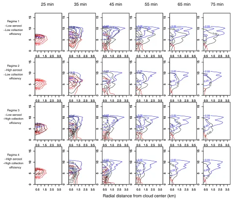
Figure 4 depicts the average simulated cloud as it develops over time from each of these defined cloud behaviors. There are visible differences in the four regimes. Generally, the graupel masses are higher in regimes of high collection efficiency (R3 versus R1 and R4 versus R2) and higher in regimes of low aerosol (R1 versus R2 and R3 versus R4). Correspondingly, precipitation is heavier in regimes of high collection effi-ciency and regimes of low aerosol. Furthermore, precipitation starts earlier in the regimes of high collection efficiency (R3 versus R1 and R4 versus R2). It is possible that the drivers of uncertainty for the model outputs of interest may be different within each of these defined regimes and also different in comparison to when we evaluate the drivers of uncertainty with respect to the whole parameter uncertainty space. This will be considered further in section 4.3.

4.2. Uncertainty in the Cloud Responses

Figure 5 shows a histogram of the uncertainty in each cloud output due to the defined parametric uncer-tainty in the MAC3 model inputs from section 2.2, generated by Monte Carlo simulation over the whole

Regime 1 −Low aerosol −Low collection efficiency 0.05 0.5 1

0.5 1.5 2.5 3.5

0

5

10

15

0.05

0.5 1.5 2.5 3.5

0

5

10

15

0.05

0.5 1.5 2.5 3.5

0 5 10 15 0.05 0.5 1 2

0.5 1.5 2.5 3.5

0 5 10 15 0.05 0.25 0.5

0.5 1.5 2.5 3.5

0 5 10 15 0.05 0.5 1 1.5

0.5 1.5 2.5 3.5

0 5 10 15 0.05 0.5 1

0.5 1.5 2.5 3.5

0 5 10 15 0.05 0.25 0.5

0.5 1.5 2.5 3.5

0 5 10 15 0.05 0.5 1 1.5 2

0.5 1.5 2.5 3.5

0

5

10

15

0.05

0.5 1.5 2.5 3.5

0

5

10

15

0.05 _0.25

0.5 1.5 2.5 3.5

0 5 10 15 0.05 0.5 1 2

0.5 1.5 2.5 3.5

0

5

10

15

0.05

0.5 1.5 2.5 3.5

0 5 10 15 0.05 0.25

0.5 1.5 2.5 3.5

0 5 10 15 0.05 0.5 1

0.5 1.5 2.5 3.5

0

5

10

15

0.05

0.5 1.5 2.5 3.5

0

5

10

15

0.05

0.5 1.5 2.5 3.5

0 5 10 15 0.05 0.5

0.5 1.5 2.5 3.5

0 5 10 15 Regime 2 −High aerosol −Low collection efficiency 0.05 0.5 1

0.5 1.5 2.5 3.5

0

5

10

15

0.5 1.5 2.5 3.5

0

5

10

15

0.5 1.5 2.5 3.5

0 5 10 15 0.05 0.5 1

0.5 1.5 2.5 3.5

0

5

10

15

0.05

0.5 1.5 2.5 3.5

0 5 10 15 0.05 0.5

0.5 1.5 2.5 3.5

0 5 10 15 0.05 0.5

0.5 1.5 2.5 3.5

0 5 10 15 0.05 0.25

0.5 1.5 2.5 3.5

0 5 10 15 0.05 0.5 1

0.5 1.5 2.5 3.5

0

5

10

15

0.05

0.5 1.5 2.5 3.5

0 5 10 15 0.05 0.25

0.5 1.5 2.5 3.5

0 5 10 15 0.05 0.5

0.5 1.5 2.5 3.5

0

5

10

15

0_.05

0.5 1.5 2.5 3.5

0 5 10 15 0.05 0.25

0.5 1.5 2.5 3.5

0

5

10

15

0.05

0.5 1.5 2.5 3.5

0

5

10

15

0.5 1.5 2.5 3.5

0 5 10 15 0.05 0.25

0.5 1.5 2.5 3.5

0 5 10 15 0.0 5

0.5 1.5 2.5 3.5

0 5 10 15 Regime 3 −Low aerosol −High collection efficiency 0.05 0.5

0.5 1.5 2.5 3.5

0

5

10

15

0.05

0.5 1.5 2.5 3.5

0 5 10 15 0.05 0.5

0.5 1.5 2.5 3.5

0 5 10 15 0.05 0.5 1

0.5 1.5 2.5 3.5

0 5 10 15 0.05 0.25

0.5 1.5 2.5 3.5

0 5 10 15 0.05 0.5 1 1.5 2 2.5

0.5 1.5 2.5 3.5

0 5 10 15 0.05 1

0.5 1.5 2.5 3.5

0 5 10 15 0.05 0.25 0.5

0.5 1.5 2.5 3.5

0 5 10 15 0.05 0.5 1 1.5 2

0.5 1.5 2.5 3.5

0

5

10

15

0.05

0.5 1.5 2.5 3.5

0 5 10 15 0.05 0.25 0.5

0.5 1.5 2.5 3.5

0 5 10 15 0.05 0.5 1

0.5 1.5 2.5 3.5

0

5

10

15

0.05

0.5 1.5 2.5 3.5

0 5 10 15 0.05 0.25

0.5 1.5 2.5 3.5

0 5 10 15 0.05 0.5

0.5 1.5 2.5 3.5

0

5

10

15

0_.05

0.5 1.5 2.5 3.5

0 5 10 15 0.05 0.25

0.5 1.5 2.5 3.5

0 5 10 15 0.05 0.5

0.5 1.5 2.5 3.5

0 5 10 15 Regime 4 −High aerosol −High collection efficiency 0.05 0.5 1

0.5 1.5 2.5 3.5

0

5

10

15

0.5 1.5 2.5 3.5

0

5

10

15

0.05

0.5 1.5 2.5 3.5

0 5 10 15 0.05 0.5

0.5 1.5 2.5 3.5

0 5 10 15 0.05 0.25

0.5 1.5 2.5 3.5

0 5 10 15 0.05 0.5 1 1.5 2

0.5 1.5 2.5 3.5

0 5 10 15 0.05 0.05 1

0.5 1.5 2.5 3.5

0 5 10 15 0.05 0.25 0.5

0.5 1.5 2.5 3.5

0 5 10 15 0.05 0.5 1

0.5 1.5 2.5 3.5

0

5

10

15

0.05

0.5 1.5 2.5 3.5

0 5 10 15 0.05 0.25 0.5

0.5 1.5 2.5 3.5

0 5 10 15 0.05 0.5 1

0.5 1.5 2.5 3.5

0 5 10 15 0_.0 5

0.5 1.5 2.5 3.5

0 5 10 15 0.05 0.25

0.5 1.5 2.5 3.5

0 5 10 15 0.05 0.5

0.5 1.5 2.5 3.5

0

5

10

15

0_.05

0.5 1.5 2.5 3.5

0 5 10 15 0.05 0.25

0.5 1.5 2.5 3.5

0

5

10

15

0.05

0.5 1.5 2.5 3.5

0

5

10

15

25 min 35 min 45 min 55 min 65 min 75 min

Radial distance from cloud center (km)

Figure 4.Time sequence of the averaged specific mass contents (g m23

) of the simulated clouds from 25 to 75 min at 10 min intervals for each of the four regimes as defined in Figure 3 and section 4.1. Thexandyaxes are radial distance from cloud center (km) and altitude (km), respectively. Red lines correspond to drops, blue lines correspond to ice crystals, and black lines correspond to graupel particles. Across the particle types, contours for mass contents of 0.05, 0.25, 0.5, 1, 1.5, 2, and 2.5 g m23

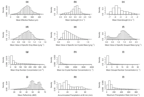
parameter uncertainty space using the emulator. Here we assume a uniform distribution across the defined range of values for each uncertain input parameter and use a sample size of 5500 input combinations in each case. The shape of the uncertainty distribution changes depending on the cloud response considered, and many of the simulated distributions show a degree of skewness. Figures 5g–5i show that the mean par-ticle number concentrations of drops, ice crystals, and graupel parpar-ticles in the cloud vary exponentially, and the range of possible values for the mean number concentration of ice crystals is extremely large. The uncertainty in the precipitation responses (Figures 5k and 5l) is positively skewed, and we also note that there is a second mode in the distribution for the accumulated precipitation at low values. This may be caused by the identified regime changes in the simulated cloud from section 4.1, with the low peak in the distribution likely corresponding to clouds from Regime R2 (Figure 3, red points) with high aerosol and low collection efficiency of drops by graupel particles.

Table 2 contains summary statistics for each output, calculated from the simulated uncertainty distributions in Figure 5. These include the minimum, lower quartile, median, upper quartile, and maximum values from the distribution, the mean value (l), and the standard deviation (r). These statistics provide an overview of the absolute uncertainty generated in each cloud response as a result of the defined uncertainty in the model input parameters, showing the absolute spread of values as well as a further indication of the amount of skewness in the output distribution given by the difference in the mean and median values. The final column gives the relative uncertainty, calculated asjr=lj, which indicates which outputs show the most variation relative to the mean value in their respective uncertainty distributions.

From both Figure 5 and Table 2, the mean drop number concentration, the mean ice crystal number con-centration, and the mean graupel number concentration are the most uncertain of the cloud responses, with values ofjr=lj>1 corresponding to a standard deviation that is greater than 100% the magnitude of the mean value. In absolute terms the mean ice number concentration is the most variable of these cloud

(a)

Mean Effective Radius (µm)

Density

0 100 200 300 400

0.000

0.005

(b)

Mean Updraught (ms−1)

Density

2.0 2.5 3.0 3.5 4.0 4.5 5.0

0.0

0

.6

(c)

Mean Downdraught (ms−1)

Density

−7 −6 −5 −4 −3 −2

0.0

0

.3

(d)

Mean Value of Specific Drop Mass (gkg−1)

Density

0.4 0.6 0.8 1.0 1.2 1.4 1.6

0.0

1

.0

2.0

(e)

Mean Value of Specific Ice Crystal Mass (gkg−1)

Density

0.0 0.5 1.0 1.5

0.0

1

.0

(f)

Mean Value of Specific Graupel Mass (gkg−1)

Density

0.0 0.5 1.0 1.5 2.0 2.5

0.0

0.6

(g)

Mean Drop Number Concentration (cm−3)

Density

0 50 100 150 200 250 300 350

0.000

0

.015

(h)

Mean Ice Crystal Number Concentration (L−1)

Density

0 1000 2000 3000 4000

0.000

0

.003

(i)

Mean Graupel Number Concentration (L−1)

Density

0 5 10 15 20 25 30

0.0

0

.2

(j)

Mean Reflectivity (dBZ)

Density

20 30 40 50 60 70

0.00

0.04

(k)

Accummulated Precipitation at 80 min (mm)

Density

0 20 40 60

0.00

0.03

(l)

Maximum Precipitation Rate (mmhour−1)

Density

0 200 400 600 800

0.000

0

.005

responses, with the range of possible values covering both extremes of a very low concentration of ice crys-tals in the cloud at a minimum value of approximately 0.5 L21, to a cloud that is completely dominated by ice crystals at a maximum value of approximately 3800 L21. However, in relative terms it is the mean grau-pel number concentration that shows the largest spread relative to the mean value, with a standard devia-tion that is more than 150% the magnitude of the mean value. The cloud response that varies the least relative to the mean value is the mean updraught. The relative uncertainty estimates for the precipitation responses indicate that there is more uncertainty across the parameter uncertainty space in the maximum precipitation rate than in the amount of accumulated precipitation at 80 min.

4.3. Sensitivity Study

To determine which factors and processes are controlling the uncertainty in the model outputs, we per-formed a variance-based sensitivity analysis with respect to each of the cloud model outputs individually. In each case, we have calculated the main effect and total effect sensitivity measures using the formulae from equations (B2) and (B4) in Appendix B, respectively.

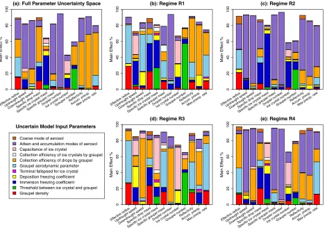
Figure 6 shows stacked bar charts of the main effect sensitivity results for the 12 model outputs when the sensitivity of the outputs is evaluated across the whole parameter space and separately in each of the regimes defined by the setting of the aerosol and collection efficiency parameters. We can infer from the plots in Figure 6 that the model output uncertainty is mainly driven by the first order main effects for the majority of the cloud responses, with at least 80% of the uncertainty attributed to main effects for around nine of the 12 outputs in each case. Where the height of the stacked bar is less than 100%, this indicates that there are interaction effects providing more significant contributions to the output uncertainty. In par-ticular, we see that this occurs for the mean value of specific ice crystal mass and the mean number

Main Eff ect % 0 2 04 06 08 0 1 0 0 Effectiv e radius Updraught speed Downdraught speedSpecific drop mass

Specific ice cr ystal mass

Specific graupel mass Droplet number Ice cr ystal number Graupel number Reflectivity Accum. precip . Max precip . rate (a): Full Parameter Uncertainty Space

Main Eff ect % 0 2 04 06 08 0 1 0 0 Effectiv e radius Updraught speed Downdraught speedSpecific drop mass

Specific ice cr ystal mass

Specific graupel mass Droplet number Ice cr ystal number Graupel number Reflectivity Accum. precip . Max precip . rate (b): Regime R1

Main Eff ect % 0 2 04 06 08 0 1 0 0 Effectiv e radius Updraught speed Downdraught speedSpecific drop mass

Specific ice cr ystal mass

Specific graupel mass Droplet number Ice cr ystal number Graupel number Reflectivity Accum. precip . Max precip . rate (c): Regime R2

Coarse mode of aerosol

Aitken and accumulation modes of aerosol Capacitance of ice crystal

Collection efficiency of ice crystals by graupel Collection efficiency of drops by graupel Graupel aerodynamic parameter Terminal fallspeed for ice crystal Deposition freezing coefficient Immersion freezing coefficient Threshold between ice crystal and graupel Graupel density

Uncertain Model Input Parameters

Main Eff ect % 0 2 04 06 08 0 1 0 0 Effectiv e radius Updraught speed Downdraught speedSpecific drop mass

Specific ice cr ystal mass

Specific graupel mass Droplet number Ice cr ystal number Graupel number Reflectivity Accum. precip . Max precip . rate (d): Regime R3

Main Eff ect % 0 2 04 06 08 0 1 0 0 Effectiv e radius Updraught speed Downdraught speedSpecific drop mass

Specific ice cr ystal mass

Specific graupel mass Droplet number Ice cr ystal number Graupel number Reflectivity Accum. precip . Max precip . rate (e): Regime R4

Figure 6.The main effect sensitivity results evaluated for all cloud responses (a) given the full parameter uncertainty space, (b) for Regime R1 (low concentration of Aitken and accumula-tion modes of aerosol,X10, and low collection efficiency of drops by graupel,X7), (c) for Regime R2 (highX10and lowX7), (d) for Regime R3 (lowX10and highX7), and (e) for Regime R4

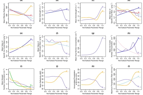
concentration of both ice crystals and graupel particles. Figure 7 displays the largest, and therefore most significant, main effects from the sensitivity analysis over the full parameter uncertainty space, showing how the model outputs are responding to the perturbation of these parameters over their uncertainty ranges. Main effects are included in Figure 7 if the corresponding contribution to the uncertainty in the model output is greater than 5%. The model output response is essentially flat for parameters not included, where the uncertainty contribution is less than 5%. Below we examine the main factors controlling uncer-tainty in the different cloud responses and we discuss the implications of these findings.

4.3.1. The Precipitation Responses

Figure 6 shows that the important contributors to the uncertainty in the maximum precipitation rate are the collection efficiency of drops by graupel, the graupel aerodynamic parameter, the concentration of the Aitken and accumulation mode aerosol, and the graupel density. Since the mass of a drop is proportional to the cube of its radius, the amount of precipitation is controlled mostly by large drops. It has been shown that the precipitation in midlatitude convective clouds is mainly due to the melting of the rimed graupel particles [Cui et al., 2011a]. The rimed mass of a graupel particle depends on the concentration of drops to be captured, the sweeping volume and the collection efficiency. The concentration of drops is generally controlled by the Aitken and accumulation modes of aerosol, whereas the sweeping volume is a function of the terminal fall speed of the graupel and the sweeping area, which are influenced by the graupel density and the graupel aerodynamic parameter.

The relative sizes of the uncertainty contributions from the different parameters varies both between the analysis over the full parameter uncertainty space (Figure 6a) and the analyses over the four separate regimes (Figures 6b–6e), and from regime to regime. When we consider the uncertainty across the full

0.0 0.2 0.4 0.6 0.8 1.0

100

2

00

300

(a)

Normalised Parameter Range

Mean Eff

e

ctiv

e Radius (

µ m) X1 X6 X7 X10

0.0 0.2 0.4 0.6 0.8 1.0

2.0 2 .5 3.0 3 .5 4.0 4 .5 (b)

Normalised Parameter Range

Mean Updraught ( ms − 1) X3 X10

0.0 0.2 0.4 0.6 0.8 1.0

−6 −5 −4 −3 −2 (c)

Normalised Parameter Range

Mean Do wndraught ( ms − 1) X7 X10

0.0 0.2 0.4 0.6 0.8 1.0

0.5 0 .7 0.9 1 .1 (d)

Normalised Parameter Range

Mean V

a

lue of

Specific Drop Mass

( gk g − 1) X1 X3 X6 X7 X10

0.0 0.2 0.4 0.6 0.8 1.0

0.2 0 .4 0.6 0 .8 1.0 (e)

Normalised Parameter Range

Mean V

a

lue of

Specific Ice Cr

ystal Mass ( gk g − 1) X3 X4 X9

0.0 0.2 0.4 0.6 0.8 1.0

0.0 0 .5 1.0 1.5 2.0 (f)

Normalised Parameter Range

Mean V

a

lue o

f

Specific Graupel Mass

( gk g − 1) X6 X7 X10

0.0 0.2 0.4 0.6 0.8 1.0

0 5 0 100 200 (g)

Normalised Parameter Range

Mean Drop Number Concentration

(

cm

−

3)

X10

0.0 0.2 0.4 0.6 0.8 1.0

0 200 400 6 00 (h)

Normalised Parameter Range

Mean Ice Cr

ystal Number Concentration ( cm − 3) X3 X9 X10

0.0 0.2 0.4 0.6 0.8 1.0

02468

(i)

Normalised Parameter Range

Mean Graupe l Number Concentration ( cm − 3) X2 X7 X10

0.0 0.2 0.4 0.6 0.8 1.0

35 40 45 50 55 60 65 (j)

Normalised Parameter Range

Mean Reflectivity (dBZ)

X7

X10

0.0 0.2 0.4 0.6 0.8 1.0

0 1 02 03 04 05 06 0 (k)

Normalised Parameter Range

Accumulated Precipitation

at 80 mins (mm)

X7

X10

0.0 0.2 0.4 0.6 0.8 1.0

0 100 200 300 400 (l)

Normalised Parameter Range

Maximum Precipitation Rate

( mm hour − 1) X6 X7 X10

Figure 7.The most significant main effects for each model output from the sensitivity analysis over the full parameter uncertainty space (Figure 6a), for which the corresponding contri-bution to the uncertainty in the model output is greater than 5%. The main effects are colored according to the legend of Figure 6, whereX1is the graupel density,X2is the threshold

between ice crystal and graupel,X3is the immersion freezing coefficient,X4is the deposition freezing coefficient,X6is the graupel aerodynamic parameter,X7is the collection efficiency

parameter space (Figure 6a), the variation in the parameter for the collection efficiency of the drops by graupel particles very much drives the uncertainty in the maximum precipitation rate. However, within each regime this parameter is much less influential. In regime R1 (Figure 6b), where the resource of aerosol to be collected is low, the main contributions to the uncertainty in the maximum precipitation rate come from the uncertainty in the sweeping volume (which is driven by the graupel aerodynamic parameter and the graupel density) as well as the collection efficiency. In regime R2 (Figure 6c), the parameter relating to the concentration of the Aitken and accumulation modes of aerosol has the largest influence on the output uncertainty, with the parameters corresponding to the collection efficiency and the sweeping volume being secondary. For regimes R3 and R4 with high collection efficiency (Figures 6d and 6e), the sweeping volume parameters provide the largest contribution to the uncertainty, with smaller contributions from the aerosol and collection efficiency.

The main drivers of the uncertainty in the accumulated precipitation at 80 min are the aerosol concentra-tion and the collecconcentra-tion efficiency, and not the graupel aerodynamic parameter or the graupel density (the sweeping volume) which most influence the uncertainty in the maximum precipitation rate. Figure 6a shows that given the full uncertainty across all input parameters, the uncertainty in the collection efficiency of drops by graupel is by far the largest contributor to the output uncertainty for the accumulated precipita-tion at 80 min, with the Aitken and accumulaprecipita-tion mode aerosol concentraprecipita-tion providing a secondary source of uncertainty. However, the contributing sources change in the different regimes. Under the low aerosol conditions in regimes R1 and R3 (Figures 6b and 6d), the collection efficiency of the drops by graupel par-ticles still dominates the output uncertainty, but the contribution from the aerosol parameter is reduced from that seen with respect to the full parameter space in Figure 6a. In contrast, under the high aerosol con-ditions in regimes R2 and R4 (Figures 6c and 6e), the concentration of the Aitken and accumulation mode aerosol provides a substantially larger contribution than the collection efficiency. We also see in Figures 6b and 6d that further input parameters make smaller contributions to the uncertainty in the accumulated pre-cipitation at 80 min within the low aerosol regimes (R1 and R3) that were not seen to be important over the full parameter uncertainty space. In particular, the two primary freezing modes represented by the immer-sion freezing coefficient and the deposition freezing coefficient show more influence within regimes R3 and R1, respectively. Under low aerosol conditions, the warm rain process is not as suppressed as in the high aerosol cases. Some large drops freeze and become graupel particles which melt after falling down below the 0_{C level and turn into rain.}

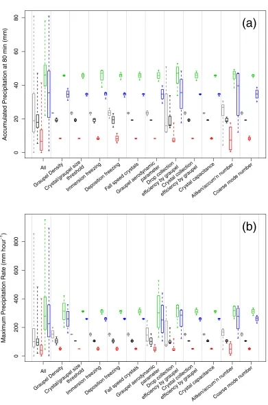
Figure 8 shows the contributions to the uncertainty in the precipitation responses as box-whisker plots. The box part represents the median and interquartile range of the simulated distribution and the whisker extends to the distribution extremes (minimum and maximum values). The ‘‘All’’ column in each plot shows the overall uncertainty in the cloud precipitation response that is due to the joint parametric uncertainty from all of the input parameters together. The high collection efficiency regimes (R3 and R4) show much more overall variability in the precipitation responses than for the low collection efficiency regimes (R1 and R2). Also, the overall uncertainty distributions across the regimes for the maximum precipitation rate response are positively skewed, with long upper tails, whereas we see much more symmetric uncertainty distributions across the regimes for the accumulated precipitation response (with the exception of regime R2 which has a very strong positive skew).

The remaining columns in Figure 8 show box plot representations of the main effect contributions to the output uncertainty from each of the uncertain input parameters in turn, where the colors are as defined for the different regimes in section 4.1 and Figure 3. For each input parameter, the main effect index is essen-tially a scaled version of the individual variance contributionVi5VarXifEX2i½YjXigto the overall decomposi-tion of variance for the model output given by equadecomposi-tion (B1) in Appendix B, where the notadecomposi-tionX2i

represents the full set of input parameters excluding parameterXi. The box and whisker plots here have

been produced by evaluating the distribution of the conditional statistical expectation over which the indi-vidual variance contributionsViare calculated,EX2i½YjXi, via simulation from the fitted emulator model. For each input parameterXi, this expectation was computed for 500 equally spaced values over the range of

the conditioning inputXi, where each of these calculations of the expectation was made using 10,000

simu-lations over the parameter space defined byX2ifor the given value ofXi. These box and whisker plots

Accumulated Precipitation at 80 min (mm)

0

2

04

06

08

0

All

Graupel Density Crystal/graupel si

ze

threshold

Immersion freezingDeposition freezingFall speed cr ystals

Graupel aerodynamic parameter

Drop collection

efficiency by graupel

Crystal collection

efficiency by graupel

Crystal capacitance Aitk

en/accum’n number Coarse mode number

(a)

Maximum Precipitation Rate (mm hour

−

1 )

0

2

00

400

6

00

800

All

Graupel Density Crystal/graupel si

ze

threshol d

Immersion freezingDeposition freezingFall speed cr ystals

Graupel aerodynamic parameter

Drop collection

efficiency by graupel

Crystal collection

efficiency by graupel

Crystal capacitance Aitk

en/accum’n number Coarse mode number

(b)

Figure 8.The individual contributions from each of the uncertain input parameters (xaxis) to the uncertainty in (a) the accumulated pre-cipitation at 80 min (Y11), and (b) the maximum precipitation rate (Y12), with respect to the full parameter uncertainty space (gray), and