Abstract: epidemiologists are often interested in examining the effect on a later-life outcome of an exposure measured repeatedly over the life course. When different hypotheses for this effect are proposed by competing theories, it is important to identify those most supported by observed data as a first step toward estimating causal associations. One method is to compare goodness-of-fit of hypothesized models with a saturated model, but it is unclear how to judge the “best” out of two hypothesized models that both pass criteria for a good fit. We developed a new method using the least absolute shrinkage and selection opera-tor to identify which of a small set of hypothesized models explains most of the observed outcome variation. We analyzed a cohort study with repeated measures of socioeconomic position (exposure) through childhood, early- and mid-adulthood, and body mass index (outcome) measured in mid-adulthood. We confirmed previous findings regard-ing support or lack of support for the followregard-ing hypotheses: accumula-tion (number of times exposed), three critical periods (only exposure in childhood, early- or mid-adulthood), and social mobility (transition from low to high socioeconomic position). Simulations showed that our least absolute shrinkage and selection operator approach identified the most suitable hypothesized model with high probability in moderately sized samples, but with lower probability for hypotheses involving change in exposure or highly correlated exposures. identifying a single, simple hypothesis that represents the specified knowledge of the life course association allows more precise definition of the causal effect of interest.
(Epidemiology 2015;26: 719–726)
M
edical research over the past two decades has examined fetal and early life antecedents of disease, and their interaction with other exposures throughout the life course to influence later-life conditions.1 Several hypothetical relationsbetween repeated covariate measures (e.g., repeated measures of socioeconomic position in childhood) and a subsequent outcome (e.g., adult blood pressure) can be proposed, based on theoretical models or mechanisms of action.2,3 For example, a
hypothesized “critical period” in early childhood specifies that socioeconomic position during this period has lasting effects on blood pressure. an alternative hypothesis is of an “accumu-lation” of risk across the life course (i.e., that adverse social circumstances at any time increases subsequent risk of high blood pressure). the hypotheses examined should inform the analytic methods used.4–6 the first step in estimating a causal
association is to specify knowledge about the system—in this case the life course—being studied.7 this knowledge will be
incomplete unless the hypothesized relation between expo-sures and outcome has been investigated. the initial investi-gation may be thought of as exploratory: determining the most likely relation, while later analyses may be thought of as con-firmatory: verifying the hypothesized relation and checking that no other relations are present.
there has been growing interest in a structured approach to life course hypotheses, in which a closed set of hypoth-eses is proposed and tests conducted to identify best-fitting hypotheses.8 One such approach uses an F test to compare
a saturated model with hypothesized models concerning the association between binary exposure variables, measured over the life course, and an outcome.9 this method has been used
in several studies with continuous outcomes10–16 and adapted
for binary outcomes.17–19 a hypothesis may be thought of as
supported by observed data if the F test yields a P value above a certain threshold, although a large P value cannot be consid-ered to “prove” the hypothesis. if more than one hypothesis passes the threshold, the hypothesis that renders the largest
P value, or smallest akaike information criterion,20,21 may be
selected. the performance of these methods in the life course setting has not been formally assessed.
We describe an alternative model selection strategy that identifies which hypothesis, selected from an a priori-compiled set of hypotheses, explains the most variation in
copyright © 2015 Wolters Kluwer Health, inc. all rights reserved. this is an open access article distributed under the creative commons attribution license, which permits unrestricted use, distribution, and reproduction in any medium, provided the original work is properly cited.
iSSn: 1044-3983/15/2605-0719 DOi: 10.1097/eDe.0000000000000348
From the aSchool of Social and community Medicine, University of Bristol,
Bristol, United Kingdom; bMrc integrative epidemiology Unit at the
University of Bristol, Bristol, United Kingdom; cSchool of Population
Health, University of Queensland, St lucia, QlD, australia; and d
Divi-sion of epidemiology and Biostatistics, School of Medicine, University of leeds, leeds, United Kingdom.
aS, JH, MSg, and Kt were supported by the Medical research council (grant number g1000726). aS and Kt work in a Unit that receives fund-ing from the UK Medical research council and the University of Bristol (Mc_UU_12013/9).
the authors report no conflicts of interest.
Supplemental digital content is available through direct Url citations in the HtMl and PDF versions of this article (www.epidem.com). this content is not peer-reviewed or copy-edited; it is the sole respon-sibility of the authors.
correspondence: andrew D. a. c. Smith, Oakfield House, Oakfield grove, Bristol BS8 2Bn, United Kingdom. e-mail: [email protected].
Model Selection of the Effect of Binary Exposures over the
Life Course
the outcome. We illustrate how the proposed method can be used in both exploratory and confirmatory studies. the per-formance is contrasted with the structured F test approach in data from a previously published example,9 and also through
simulation.
METHODS
the proposed strategy involves selecting from an a pri-ori-compiled set of potential hypotheses describing the asso-ciation between exposure over the life course and outcome. each hypothesis is encoded into one or more variables, which are then all included in a regression model, and the subset of variables that explains the greatest proportion of the out-come variation is selected. the number of hypotheses is not limited; any hypothesis may be examined provided there are enough exposure measurements to identify it. Several varia-tions of similar hypothesis may be considered (e.g., a set of critical period hypotheses covering a range of possibly over-lapping periods). the choice of hypotheses to examine may be informed by knowledge of causal mechanisms, perhaps using a directed acyclic graph. examples of typical hypotheses for binary exposures are described below.
an accumulation hypothesis states that there is a linear association between the outcome and the cumulative sum of the exposure over the life course.
a critical period hypothesis states that only exposure during one period is associated with the outcome. Under a
sensitive period hypothesis, the outcome is associated with the
amount of exposure, as in the accumulation hypothesis, but the association is stronger in a particular period.21
a mobility hypothesis states that the outcome is asso-ciated with changes in the exposure over time. the simplest mobility hypotheses relate the outcome only to unidirectional changes. a more complex mobility hypothesis may relate the outcome to bidirectional changes9,22 (e.g., a positive
associa-tion with increased exposure and a negative associaassocia-tion with decreased exposure). this would in general enhance the plau-sibility of a causal association. the related interaction hypoth-esis states that the outcome is associated with the exposure in a particular period, but that this association is altered by the exposure in a different period.
Encoding of Variables
each hypothesis is encoded as a variable that is pro-portional to the hypothesized outcome as the exposure var-ies. Simpler hypotheses may be encoded by a single variable; more complex hypotheses need multiple variables. Below, we give details of the single variables that encode the simple hypotheses discussed above. We assume a set of m repeated binary measures of exposure X1,...,Xm.
the accumulation hypothesis is encoded by the variable
A = X1 +…+ Xm.
if there is only one measurement occasion during a hypothesized critical period then only that measurement will
be associated with the outcome. a hypothesis of a critical period at the jth measurement occasion is encoded by the vari-able Cj = Xj. if there are several measurement occasions dur-ing the critical period (e.g., Xj,...,Xk), then the critical period hypothesis may be encoded by Cjk = Xj +…+ Xk, i.e., as accu-mulation within the critical period.
Under the simplest mobility hypothesis, the outcome varies with a unidirectional change in the exposure. a mobil-ity hypothesis between the jth and kth measurement occasions may be encoded by Mjk+ = (1 − X
j)Xk if it is hypothesized that
a positive change from j to k is associated with the outcome, or by M−jk= X
j(1 − Xk) if it is hypothesized that a negative change
from j to k is associated with the outcome.
Some hypotheses require more than one variable to encode, and can therefore be thought of as compound hypoth-eses. all of these can be encoded by combinations of variables encoding simple hypotheses; some quite complex hypotheses can be encoded with two variables. the combinations of vari-ables that encode compound hypotheses are described below, with further details provided in eappendix a (http://links. lww.com/eDe/a940).
a sensitive period hypothesis can be encoded by the combination of the accumulation variable and the relevant critical period variable.
two simple mobility variables can, together, encode a more complex mobility hypothesis. For instance, mobility hypotheses may combine a variable encoding positive change with a variable encoding negative change, or variables encod-ing change at different pairs of measurement occasions over the life course.9 an interaction hypothesis can be encoded by
combining critical period and mobility variables. For example, combining the critical period variable Cj with mobility vari-able Mjk+ encodes a hypothesis that the outcome is associated with the exposure measurement at occasion j, but this associa-tion is modified by the exposure measurement at occasion k. Choosing Hypotheses Most Strongly Supported by Observed Data
after encoding potential hypotheses, our approach is to examine the association between all encoded variables and the outcome, and select only those encoded variable combinations that have the strongest association with the outcome. Since there are potentially more variables than available degrees of freedom it is inappropriate to put all encoded hypotheses into a linear model and choose the variable(s) with the largest parameter estimates. instead, we propose placing an absolute value penalty on parameter estimates, whereby unimportant variables have their estimated association shrunk to zero. Hence, the resulting fit will provide the fullest explanation of the observed data from the fewest parameters. the least absolute Shrinkage and Selection Operator (lasso),23 which
the least angle regression (larS) approach to the lasso,24
which provides lasso estimates for all smoothing parameter values and indicates the best lasso fit for each number of selected variables, reducing the problem to that of choosing the number of variables. the lasso is a constrained version of linear regression and may be used whenever the assump-tions of linear regression are satisfied. the larS algorithm first selects the variable with the strongest association with the outcome,25 hence this approach will always select first
the hypothesis, or component of a compound hypothesis, that offers the strongest explanation for the observed data. Using an absolute value penalty causes subsequent variables to be added in order of strength of association with outcome varia-tion.26 the overall hypothesized view of the data is thus built
from the most relevant simple hypotheses or components of compound hypotheses.
When little is known regarding the association between the exposures and outcome over the life course, the struc-tured approach can be used to suggest the most likely of an a priori-defined set of hypothesized associations. this set may extend to several hypotheses if we have little a priori infor-mation about which are likely. in this exploratory setting, the choice of hypothesis is somewhat subjective and we require a method for choosing how many variables to include in our selected hypothesis. We use an elbow plot—a plot of the pro-portion of outcome variation explained by the lasso fit (the R2
value) against number of variables selected at each stage in the larS procedure. the “elbow”—a sharp concave bend at which adding more variables does not substantially increase the R2 value—is used to choose the number of variables.
Pro-vided enough variables are included in the procedure, the elbow plot will show how the lasso selections approach a saturated model. it is useful to see the R2 value for a saturated
model to check whether there is any association between the outcome and all exposure measurements over the life course. an alternative method for selecting the number of variables is provided by the lasso covariance hypothesis test.27 at each
stage of the larS procedure, this tests the null hypothesis that adding the next variable does not improve the R2 value.
the covariance hypothesis test accounts for the fact that the next variable will have the greatest association out of the variables not already selected. an alternative option, a nested
F test to discriminate between simple and complex
hypoth-eses,22 may be biased by the selection of the simpler model
due to its greater association. in the exploratory setting, it may be necessary to reject more compound hypotheses in favor of simpler ones to maintain plausibility.
We may have a firmer idea of the nature of the life course association between exposures and outcome, and perhaps some causal information. in this setting, we might specify quite a small number of possible hypotheses a pri-ori, and rather than choose the number of variables in our selected hypothesis we might simply choose the first variable
or hypothesis selected by the larS algorithm, to confirm our causal assumptions.
EXAMPLE
the proposed approach, in the exploratory setting, is illustrated using data on socioeconomic position and body mass index (BMi) from a cohort of 2,192 men and women, with binary measurements of the exposure, socioeconomic position, at ages 4, 26, and 43 years, and a continuous mea-surement of the outcome, BMi, at age 53 years. these data were previously used to illustrate the structured approach, and full details are given in the original study.9 issues such
as confounding and measurement error were not the focus of the original study and are therefore ignored here for sake of simplicity and comparison with the alternative structured method. Figure 1 shows a possible directed acyclic graph for this example. While there are many potential confounders of the life course association between exposure and outcome, which in this example are unmeasured (as they were in the original study), the focus in this exploratory setting is to iden-tify likely life course associations between exposure and out-come, whether or not they are confounded. We considered the set of six hypotheses that have been previously proposed for this data: three critical period hypotheses corresponding to the three exposure measurement occasions, two mobility hypoth-eses concerning change between adjacent measurement occa-sions, and an accumulation hypothesis.9
Encoding of Variables
each hypothesis was encoded based on the binary expo-sure meaexpo-surements X1, X2, and X3 at the three time points, where zero represents a manual socioeconomic position and one a nonmanual socioeconomic position. the simple hypoth-eses, requiring one variable each, were the three critical period hypotheses, encoded by C1, C2, and C3, and the accumulation hypothesis, encoded by A = X1 + X2 + X3. the two mobility hypotheses required two variables each, with M12+ and M
12−
encoding mobility between ages 4 and 26 years, and M23+ and M23− encoding mobility between ages 26 and 43 years. Use of Elbow Plot
Figure 2 shows the elbow plot for men. the variance explained by the model with the greatest number of variables was 1.7%, which approached the 2% explained by the satu-rated model; hence the maximum R2 value on the plot is close
to the maximum R2 value achievable. there is a clear elbow
where one variable is selected; adding additional variables did not considerably improve the R2 value. in addition, the P value
for adding a second variable was 0.90, indicating no evidence that one variable was insufficient. the first variable selected encoded the hypothesis of an age 4 critical period; choosing this elbow point identified this hypothesis as offering the best explanation for the observed data in men.
was 3.9%. therefore, socioeconomic position explained a greater proportion of the BMi variation in women than men. the position of an elbow point was less clear for women. the first variable selected encoded the accumulation hypothesis; the P value for adding a second variable was 0.52. it could thus be concluded that the accumulation hypothesis is the pri-mary explanation for the observed data in women. the plot might also be considered to have an elbow at three variables, selecting variables that encoded the accumulation, childhood critical period, and adult nonmanual to manual mobility vari-ables. Our interpretation of this is a hypothesis of two sensi-tive periods: sensitivity (to manual socioeconomic position) in childhood and sensitivity to change (from nonmanual to manual socioeconomic position) in adulthood.
in the exploratory setting, further study would be required to clarify these hypotheses and examine causal mechanisms.
SIMULATION STUDY
to investigate how frequently the larS algorithm selects the correct hypothesis in a confirmatory setting, we simulated data with two and three repeated binary exposures. the performance indicator is the selection probability: the proportion of simulations where the correct hypothesis is identified.
Two Exposure Measurements
two exposure measurements were simulated as binary random variables, being zero or one with equal probability (see eappendix B for details; http://links.lww.com/eDe/ a940). We considered the situation in which the outcome is known to be associated with change in the exposure, but it is yet to be confirmed whether a mobility or interaction hypoth-esis defines the true association. We simulated mobility and interaction models, varying the correlation, ρ, between expo-sure variables, and the residual variance, σ2. in each
simula-tion, we selected from six proposed compound hypotheses (four interaction hypotheses, full mobility, and an additive model).
We compared three approaches for identifying the hypotheses offering the best explanation for the simu-lated data. the first was the larS algorithm for the lasso, which was considered to have identified the correct hypothesis if the first two selected variables encoded that hypothesis. the second approach chose the hypothesized model with the largest F test P value when compared with the saturated model,9 and the third approach selected the
hypothesized model yielding the smallest akaike infor-mation criterion of those models with an F test P value not less than 0.05.21
We varied the sample size from 400, which might rep-resent a subset of a study, to 2,500, which might reprep-resent a moderate-sized study. We ran 500 simulations for each com-bination of residual variance, correlation, model, and sample
size. With 500 simulations, the 95% confidence interval for the selection probability will have a radius of less than 2% for a selection probability of 95%, and less than 5% for a selec-tion probability of 50%.
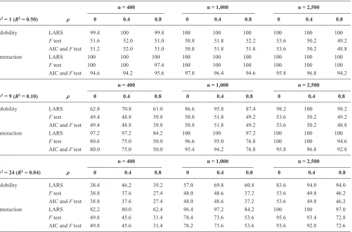
table 1 shows the selection probabilities, in simulation, of the three methods. the selection probability of the larS algorithm is very good in situations with low residual vari-ance or large sample size: it was at least 83.6% when the R2
value was at least 100/n. this approach always outperformed the alternative methods, except for a difference of 0.4% in one situation with the largest residual variance and smallest sample size.
Three Exposure Measurements
this hypothetical example considered that prior knowl-edge provided evidence for either a critical or a sensitive period; the aim being to confirm the correct association using new data. three measurements were simulated as binary variables as before, with adjacent measurements having correlations of ρ, and the first and last measurements having correlation ρ2. the models used to generate the outcome were: an early
critical period, an accumulation model, and an early sensitive period model. the simple hypotheses that the larS algo-rithm was allowed to choose from were three critical period hypotheses and an accumulation hypothesis. the larS algo-rithm was considered to have chosen a simple hypothesis if it first selected the variable encoding that hypothesis, and the covariance test P value for including another variable was not less than 0.05. the larS algorithm was considered to have identified a compound hypothesis if the first two selected vari-ables encoded that hypothesis and the P value for including the second variable was less than 0.05. While we do not neces-sarily advocate using P value thresholds to select hypotheses, this allowed comparisons with other approaches. the other two approaches used the F test and akaike information cri-terion as before, choosing between an accumulation model, three critical period models and three sensitive period models.
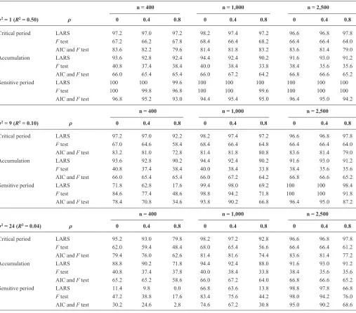
there was some evidence that selection probabilities decreased as the exposure correlation increased (table 2). the selection probability of the larS algorithm was very good with low residual variance or large sample size: it was at least 90.2%, and higher than that of other methods, when the R2
value was at least 100/n. the only exception to this was in sensitive period simulations with strong exposure correlation, where there was less distinction between accumulation and critical period hypotheses. the alternative methods had bet-ter selection probabilities in compound models than simple models; it appears that akaike information criterion or F test selection is more likely to select compound hypotheses over simple ones, regardless of the true underlying model.
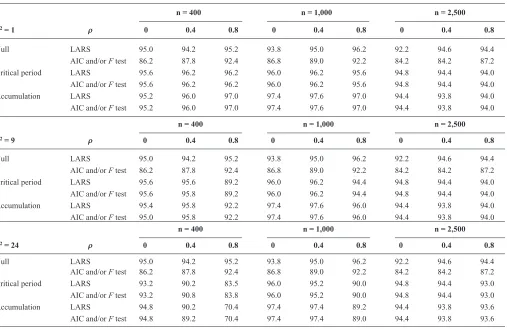
Confidence Intervals
95% confidence interval for the regression parameter in the hypothesized model with the largest F test P value (coinciden-tally the model with smallest akaike information criterion) when compared with the saturated model. We also calculated an adjusted confidence interval based on the covariance test for the lasso (see eappendix B for details; http://links.lww. com/eDe/a940). table 3 shows the coverage of these confi-dence intervals. in the null model, the coverage of the usual confidence intervals was always less than 95%, showing that the F test or akaike information criterion approach generates bias due to the fact that they consider the largest observed association to be selected at random. However, the adjusted confidence intervals have coverage between 92.2% and 96.2% in the null model, confirming that the covariance test corrects for selection of the variable with greatest association.
DISCUSSION
a causal life course association between exposure and outcome cannot be estimated without identifying knowledge of the system being studied.7 this can be achieved by
assess-ing prespecified competassess-ing hypotheses regardassess-ing that system
and the life course association. We have described a strat-egy for this, which involves encoding a set of hypotheses as covariates, and then using the larS procedure for the lasso to identify the most appropriate covariate subset that accounts for the outcome variation. Variable selection is aided visually with an elbow plot, or guided by a hypothesis test. We showed that, for one example dataset, the larS procedure identified the same hypotheses as earlier research using a structured approach.9 Furthermore, simulation showed, for reasonably
large sample sizes, the larS algorithm, even when com-bined with a naive P value threshold, effectively identified the correct hypotheses. alternative methods, based on F tests and akaike information criterion, did not identify the correct hypotheses as often and were more likely to favor compound hypotheses over simple ones.
[image:5.585.40.549.95.431.2]Our proposed approach is part of the process toward estimation of causal effects. the set of hypotheses proposed a priori can be chosen using previous knowledge and theory regarding the plausibility of various hypotheses. We have demonstrated techniques for choosing the best-fitting of those hypotheses, which can then be further investigated both for
TABLE 1. Percentage of 500 Simulations in Which the Correct Model Was Identified, in Simulations with Two Binary Exposure Measurements, by Three Different Structured Approaches
σ2 = 1 (R2 = 0.50) ρ
n = 400 n = 1,000 n = 2,500
0 0.4 0.8 0 0.4 0.8 0 0.4 0.8
Mobility larS 99.4 100 99.8 100 100 100 100 100 100
F test 51.6 52.0 51.0 50.8 51.8 52.2 53.6 50.2 49.2
aic and F test 51.2 52.0 51.0 50.8 51.8 51.8 53.6 50.2 48.8
interaction larS 100 100 100 100 100 100 100 100 100
F test 100 100 97.4 100 100 100 100 100 100
aic and F test 94.6 94.2 95.6 97.8 96.4 94.6 95.8 96.8 94.2
σ2= 9 (R2= 0.10) ρ
n = 400 n = 1,000 n = 2,500
0 0.4 0.8 0 0.4 0.8 0 0.4 0.8
Mobility larS 62.8 70.8 61.0 86.6 95.8 87.4 98.2 100 98.2
F test 49.4 48.8 39.8 50.8 51.8 49.2 53.6 50.2 49.2
aic and F test 49.4 48.8 39.8 50.8 51.8 49.2 53.6 50.2 48.8
interaction larS 97.2 97.2 84.2 100 100 97.2 100 100 100
F test 80.6 75.0 50.0 96.6 95.0 76.8 100 100 94.6
aic and F test 80.0 75.0 50.0 95.4 94.2 76.8 95.8 96.8 92.8
σ2= 24 (R2= 0.04) ρ
n = 400 n = 1,000 n = 2,500
0 0.4 0.8 0 0.4 0.8 0 0.4 0.8
Mobility larS 38.4 46.2 39.2 57.0 69.8 60.8 83.6 94.0 94.0
F test 38.8 37.6 27.4 48.0 48.6 37.2 53.6 49.8 46.2
aic and F test 38.8 37.6 27.4 48.0 48.6 37.2 53.6 49.8 46.2
interaction larS 82.2 80.0 62.4 96.4 97.2 84.2 100 100 97.0
F test 49.8 45.6 31.4 78.4 73.6 53.6 95.6 93.4 72.8
aic and F test 49.8 45.6 31.4 78.2 73.6 53.6 93.6 92.0 72.6
replication and to estimate causal effects. advantages of the structured approach are that it requires the hypotheses to be carefully specified a priori, and can accommodate complex compound hypotheses that involve interactions. For exam-ple, Forsdahl28 argued that a poor standard of living in early
years followed by later life prosperity would increase the risk of arteriosclerotic disease. in this example, the highest risk would be seen in those who change exposure between ear-lier and later time periods. Other hypotheses, such as nonlin-ear accumulation, can also be investigated. the flexibility of our approach allows many hypotheses even if they are epi-demiologically implausible: it is important to triangulate the
statistical findings with knowledge about biological and social plausibility. if suggested hypotheses are thought to be “too complex,” our procedure allows for retreat to simpler, more interpretable, hypotheses if necessary. in further investigation, only the identified hypothesis need be considered, allowing precise definition of the causal effect(s) of interest and reduc-ing their number, leadreduc-ing to improved estimation by marginal structural or structural nested models.7,29
[image:6.585.41.548.94.540.2]Our approach has the advantage that the selected hypoth-esis will always be easy to interpret, provided that interpre-table hypotheses are proposed a priori. this is in contrast to methods that provide a plot and invite interpretation based on
TABLE 2. Percentage of 500 Simulations in Which the Correct Model Was Identified, in Simulations with Three Binary Exposure Measurements, by Three Different Structured Approaches
σ2 = 1 (R2 = 0.50) ρ
n = 400 n = 1,000 n = 2,500
0 0.4 0.8 0 0.4 0.8 0 0.4 0.8
critical period larS 97.2 97.0 97.2 98.2 97.4 97.2 96.6 96.8 97.8
F test 67.2 66.2 67.8 68.4 66.4 68.2 66.4 66.4 64.0
aic and F test 83.6 82.2 79.6 81.4 81.8 83.2 83.6 81.4 79.0
accumulation larS 93.6 92.8 92.4 94.4 92.4 90.2 91.6 93.0 91.2
F test 40.8 37.4 38.4 40.0 38.4 33.8 38.4 35.6 35.6
aic and F test 66.0 65.4 65.4 66.0 67.2 64.2 66.8 66.6 65.2
Sensitive period larS 100 100 99.6 100 100 100 100 100 100
F test 100 99.8 96.8 100 100 99.6 100 100 100
aic and F test 96.8 95.2 93.0 94.4 95.4 95.0 96.4 95.0 94.2
σ2= 9 (R2= 0.10) ρ
n = 400 n = 1,000 n = 2,500
0 0.4 0.8 0 0.4 0.8 0 0.4 0.8
critical period larS 97.2 97.0 92.2 98.2 97.4 97.2 96.6 96.8 97.8
F test 67.0 64.6 58.4 68.4 66.4 64.8 66.4 66.4 64.0
aic and F test 83.2 81.0 72.8 81.4 81.8 80.8 83.6 81.4 79.0
accumulation larS 93.6 92.8 90.2 94.4 92.4 90.2 91.6 93.0 91.2
F test 40.8 37.4 38.4 40.0 38.4 33.8 38.4 35.6 35.6
aic and F test 66.0 65.4 65.4 66.0 67.2 64.2 66.8 66.6 65.2
Sensitive period larS 71.8 62.8 17.6 99.4 98.0 69.2 100 100 98.4
F test 84.6 77.4 48.6 98.8 94.2 71.8 100 100 91.8
aic and F test 78.4 70.8 34.6 93.8 90.2 66.8 96.4 95.0 87.2
σ2= 24 (R2= 0.04) ρ
n = 400 n = 1,000 n = 2,500
0 0.4 0.8 0 0.4 0.8 0 0.4 0.8
critical period larS 95.2 93.0 79.8 98.2 97.2 92.8 96.6 96.8 97.8
F test 62.0 59.4 48.4 68.0 65.4 56.6 66.4 66.4 61.2
aic and F test 79.4 76.0 62.6 81.4 81.6 74.4 83.6 81.4 77.2
accumulation larS 88.8 90.2 71.8 94.4 92.4 88.0 91.6 93.0 91.2
F test 40.8 37.4 37.8 40.0 38.4 33.8 38.4 35.6 35.6
aic and F test 65.2 65.2 58.6 66.0 67.2 64.0 66.8 66.6 65.2
Sensitive period larS 11.4 9.8 0.0 66.8 63.6 13.8 98.8 97.8 66.8
F test 47.2 38.8 17.6 83.4 75.6 44.2 98.0 94.2 76.0
aic and F test 30.2 24.6 2.8 74.6 67.2 30.8 95.0 90.2 68.6
curves on the graph.3,4 the larS algorithm has the advantage
of choosing the most important hypothesis first: that corre-sponding to the greatest proportion of the variability in the outcome, while unimportant effects are deselected. Unlike the structured F test approach,9 our approach can be employed
without using P values. Using the covariance test for the lasso, we calculated confidence intervals with coverage unaffected by the fact that the selected hypothesis offers the best fit to the observed data. the covariance test for the lasso should be used in preference to an F test between simple and compound hypothesized models.
if the association between exposure and outcome is weak, with little variation in the outcome explained by the exposure, then the reliability of structured approaches in iden-tifying the true model is diminished. it is therefore important first to examine the overall amount of variation explained by the exposure, perhaps using the R2 value in a saturated model
or extreme end of the elbow plot, and second to examine the correlation structure among the exposure measurements. if exposure measurements are highly correlated, it may be impossible to distinguish hypotheses without a large sample size or many repeated measures. additional study is required
to extend this approach to continuous exposures and categori-cal outcomes, consider measurement error in the exposure, and accommodate possible confounding.
Within the same overall structure, other variable selec-tion methods might be used instead of the lasso. One possibil-ity is the elastic net,30 although this could select more variables
than parameters in the saturated model, which would not be an advantage in understanding the hypothesized life course asso-ciation, as less parsimonious models are less interpretable. the grouped lasso would allow all variables encoding a com-pound hypothesis to be selected at the same time,31 and
pre-vent only one component variable of a compound hypothesis being identified on its own. However, if compound hypoth-eses are misspecified, for example not all of their components are associated with the outcome, then not grouping variables still allows the important components to be extracted and the hypothesis to be identified.
[image:7.585.42.549.92.421.2]Our conclusion is that the larS procedure, imple-menting the lasso, can select hypotheses from a prespecified set, identifying the optimal hypothesis that offers the great-est consistency with the data. compound hypotheses can be built from simpler hypotheses in a straightforward way, using
TABLE 3. Percentage of 500 Simulations in Which a 95% Confidence Interval Contained the True Parameter Value, in Simulations with Three Binary Exposure Measurements, Calculated by Two Different Structured Approaches
σ2 = 1 ρ
n = 400 n = 1,000 n = 2,500
0 0.4 0.8 0 0.4 0.8 0 0.4 0.8
null larS 95.0 94.2 95.2 93.8 95.0 96.2 92.2 94.6 94.4
aic and/or F test 86.2 87.8 92.4 86.8 89.0 92.2 84.2 84.2 87.2
critical period larS 95.6 96.2 96.2 96.0 96.2 95.6 94.8 94.4 94.0
aic and/or F test 95.6 96.2 96.2 96.0 96.2 95.6 94.8 94.4 94.0
accumulation larS 95.2 96.0 97.0 97.4 97.6 97.0 94.4 93.8 94.0
aic and/or F test 95.2 96.0 97.0 97.4 97.6 97.0 94.4 93.8 94.0
σ2= 9 ρ
n = 400 n = 1,000 n = 2,500
0 0.4 0.8 0 0.4 0.8 0 0.4 0.8
null larS 95.0 94.2 95.2 93.8 95.0 96.2 92.2 94.6 94.4
aic and/or F test 86.2 87.8 92.4 86.8 89.0 92.2 84.2 84.2 87.2
critical period larS 95.6 95.6 89.2 96.0 96.2 94.4 94.8 94.4 94.0
aic and/or F test 95.6 95.8 89.2 96.0 96.2 94.4 94.8 94.4 94.0
accumulation larS 95.4 95.8 92.2 97.4 97.6 96.0 94.4 93.8 94.0
aic and/or F test 95.0 95.8 92.2 97.4 97.6 96.0 94.4 93.8 94.0
σ2= 24 ρ
n = 400 n = 1,000 n = 2,500
0 0.4 0.8 0 0.4 0.8 0 0.4 0.8
null larS 95.0 94.2 95.2 93.8 95.0 96.2 92.2 94.6 94.4
aic and/or F test 86.2 87.8 92.4 86.8 89.0 92.2 84.2 84.2 87.2
critical period larS 93.2 90.2 83.5 96.0 95.2 90.0 94.8 94.4 93.0
aic and/or F test 93.2 90.8 83.8 96.0 95.2 90.0 94.8 94.4 93.0
accumulation larS 94.8 90.2 70.4 97.4 97.4 89.2 94.4 93.8 93.6
aic and/or F test 94.8 89.2 70.4 97.4 97.4 89.0 94.4 93.8 93.6
a small number of variables. the selected hypothesis and its potential causality may then be more precisely defined and further studied.
ACKNOWLEDGMENTS
The authors are grateful to the MRC Unit for Lifelong Heath and Ageing at University College London for providing the data used as an example.
REFERENCES
1. Barker DJ, Osmond c, Forsén tJ, Kajantie e, eriksson Jg. trajectories of growth among children who have coronary events as adults. N Engl J
Med. 2005;353:1802–1809.
2. Ben-Shlomo Y, Kuh D. a life course approach to chronic disease epide-miology: conceptual models, empirical challenges and interdisciplinary perspectives. Int J Epidemiol. 2002;31:285–293.
3. De Stavola Bl, nitsch D, dos Santos Silva i, et al. Statistical issues in life course epidemiology. Am J Epidemiol. 2006;163:84–96.
4. tilling K, Howe lD, Ben-Shlomo Y. commentary: methods for analys-ing life course influences on health–untanglanalys-ing complex exposures. Int J
Epidemiol. 2011;40:250–252.
5. tu YK, tilling K, Sterne Ja, gilthorpe MS. a critical evaluation of statistical approaches to examining the role of growth trajectories in the developmental origins of health and disease. Int J Epidemiol. 2013;42:1327–1339.
6. liu S, Jones rn, glymour MM. implications of lifecourse epidemiol-ogy for research on determinants of adult disease. Public Health Rev. 2010;32:489–511.
7. Petersen Ml, van der laan MJ. causal models and learning from data: integrating causal modeling and statistical estimation. Epidemiology. 2014;25:418–426.
8. Pollitt ra, rose KM, Kaufman JS. evaluating the evidence for models of life course socioeconomic factors and cardiovascular outcomes: a sys-tematic review. BMC Public Health. 2005;5:7.
9. Mishra g, nitsch D, Black S, De Stavola B, Kuh D, Hardy r. a structured approach to modelling the effects of binary exposure variables over the life course. Int J Epidemiol. 2009;38:528–537.
10. gustafsson Pe, Janlert U, theorell t, Westerlund H, Hammarström a. Fetal and life course origins of serum lipids in mid-adulthood: results from a prospective cohort study. BMC Public Health. 2010;10:484. 11. Birnie K, Martin rM, gallacher J, et al. Socio-economic disadvantage
from childhood to adulthood and locomotor function in old age: a life-course analysis of the Boyd Orr and caerphilly prospective studies.
J Epidemiol Community Health. 2011;65:1014–1023.
12. Murray et, Mishra gD, Kuh D, guralnik J, Black S, Hardy r. life course models of socioeconomic position and cardiovascular risk factors: 1946 birth cohort. Ann Epidemiol. 2011;21:589–597.
13. Park MH, Sovio U, Viner rM, Hardy rJ, Kinra S. Overweight in childhood, adolescence and adulthood and cardiovascular risk in later life: pooled analysis of three british birth cohorts. PLoS One. 2013;8:e70684.
14. evans J, Melotti r, Heron J, et al. the timing of maternal depressive symptoms and child cognitive development: a longitudinal study. J Child
Psychol Psychiatry. 2012;53:632–640.
15. Kakinami l, Séguin l, lambert M, gauvin l, nikiema B, Paradis g. comparison of three lifecourse models of poverty in predicting cardio-vascular disease risk in youth. Ann Epidemiol. 2013;23:485–491. 16. richmond rc, Simpkin aJ, Woodward g, et al. Prenatal exposure to
maternal smoking and offspring Dna methylation across the lifecourse: findings from the avon longitudinal Study of Parents and children (alSPac). Hum Mol Genet. 2015;24:2201–2217.
17. Pearson rM, Melotti r, Heron J, et al. Disruption to the development of maternal responsiveness? the impact of prenatal depression on mother-infant interactions. Infant Behav Dev. 2012;35:613–626.
18. Wills aK, Black S, cooper r, et al. life course body mass index and risk of knee osteoarthritis at the age of 53 years: evidence from the 1946 British birth cohort study. Ann Rheum Dis. 2012;71:655–660.
19. Delgado-angula eK, Bernabé e. comparing lifecourse models of social class and adult oral health using the 1958 national child Development Study. Community Dent Hlth. 2015;32:20–25.
20. akaike H. a new look at the statistical model identification. IEEE
Transacton Automat Control. 1974;19:716–723.
21. Mishra gD, chiesa F, goodman a, De Stavola B, Koupil i. Socio-economic position over the life course and all-cause, and circulatory dis-eases mortality at age 50-87 years: results from a Swedish birth cohort.
Eur J Epidemiol. 2013;28:139–147.
22. Preston SH, Mehta nK, Stokes a. Modeling obesity histories in cohort analyses of health and mortality. Epidemiology. 2013;24:158–166. 23. tibshirani r. regression shrinkage and selection via the lasso. J R Stat
Soc Ser B. 1996;58:267–288.
24. efron B, Hastie t, Johnstone i, tibshirani r. least angle regression. Ann
Stat. 2004;32:407–499.
25. radchenko P, James gM. improved variable selection with forward-lasso adaptive shrinkage. Ann Appl Stat. 2011;5:427–448.
26. Davies Pl, Kovac a. local extremes, runs, strings and multiresolution.
Ann Stat. 2001;29:1–65.
27. lockhart r, taylor J, tibshirani r, tibshirani r. a significance test for the lasso. Ann Stat. 2014;42:413–468.
28. Forsdahl a. are poor living conditions in childhood and adolescence an important risk factor for arteriosclerotic heart disease? Br J Prev Soc
Med. 1977;31:91–95.
29. robins JM, Hernán Ma, Brumback B. Marginal structural models and causal inference in epidemiology. Epidemiology. 2000;11:550–560. 30. Zou H, Hastie t. regularization and variable selection via the elastic net.
J R Stat Soc Ser B. 2005;67:301–320.