Edge Detection Using Distinct Particle Swarm Optimization

International Journal of Innovative Technology and Exploring Engineering (IJITEE) ISSN: 2278-3075, Volume-8 Issue-9, July 2019

Edge Detection Using Distinct Particle Swarm

Optimization

Naveen Singh Dagar, Pawan Kumar Dahiya

Abstract— Edge detection is long-established in computer perception approach such as object detection, shape matching, medical image classification etc. For this reason many edge detectors like, Sobel, Robert, Prewitt, Canny etc. has been progressed to increase the effectiveness of the edge pixels. All these approaches work fine on images having minimum variation in intensity. Therefore, a new objective function based distinct particle swarm optimization (DPSO)is proposed in this paper to identify unbroken edges in an image. The conventional edge detectors such as “Canny” & computational intelligent techniques like ACO, GA and PSO are compared with proposed algorithm. Precision, Recall & F-Score is used as performance parameters for these edge detection techniques. The ground truth images are taken as reference edge images and all the edge images acquired by different edge detection systems are contrasted with reference edge image with ascertain the Precision, Recall and F-Score. The techniques are tested on 500 test images from the “BSD500” datasets. The empirical results presented by the proposed algorithm performance better than other edge detection techniques in the images. The proposed method observes edges more accurately and smoothly than other edge detection techniques such as “Canny, ACO, GA and PSO” in different images.

Keyword: Image Processing, Edge Detection, Distinct Particle Swarm Optimization, BSD500, ACO, GA, PSO, F-Score.

I. INTRODUCTION

The role of “edge detection technique is important in computer eyesight. The partitions between different areas in an image are explained by an edge, which help in segmentation and recognition of objects in an image. Edge detection used to show where the boundary of the object in an image or definite change related to intensity of an image. For low level of image processing edge detection is the basic step [1]. Edge detectors don’t function up to the mark while their conduct may fall inside resilience’s in particular circumstances, when all is said in done edge detectors experience issues adjusting to various circumstances. The nature of edge recognition is very subject to blistering conditions, the nearness of objects of comparative powers, thickness of edges in the site, and commotion. These concerns can be dealt with by modifying certain qualities in the edge detector and changing the edge an incentive for what is viewed as an edge, no great technique has been resolved for naturally setting these qualities, so they should be physically changed by an administrator each time the identifier is kept running with an alternate arrangement of information. Dissimilar sorts of administrators are accessible for edge location. In any case, these administrators are grouped into two classes.”

Revised Manuscript Received on July 05, 2019.

Naveen Singh Dagar, research scholar at DeenbandhuChhotu Ram University of Science & Technology, Murthal, Sonepat, Haryana, India.

Pawan Kumar Dahiya, Assistant Professor in Electronics & Communication Engineering Department in DeenbandhuChhotu Ram University of Science & Technology, Murthal, Sonepat, Haryana, India.

In First request subordinate [2] the information picture is convolved by an adjusted cover to produce an inclination picture in that edges are distinguished by thresholding. Most established detectors like “Sobel, Prewitt and Robert [5]” are the primary request subsidiary administrators. These administrators are additionally said as slope administrators. These inclination administrators distinguish edges by searching for most extreme and least force esteems. These administrators inspect the conveyance of force esteems in the area of a given pixel and decide whether the pixel is to be named an edge. These administrators have more computational time and can't be utilized continuously application.

In second order derivatives [4], these depend on the extraction of zero crossing focuses that shows the nearness of maxima in picture. In this, picture is first smoothed by a versatile channel [5]. Since the second order derivatives is extremely sensible to noise, and the sifting capacity is vital. These administrators are gotten from the “Laplacian of a Gaussian (LOG)”, and proposed by Marr and Hildreth [6],” in this, the picture is smoothed by a Gaussian channel. For this administrator we need to settle a few parameters, for example, the fluctuation of the “Gaussian channel” and limits. A few strategies are accessible for their programmed calculation [7], however as a rule their qualities must be settled by the client.

In any case, this will generously build the calculation time. In this way an interested computation is needed to study the significant area to beat the noise\commotion and think about the universal edge structure to reduce the broken edges in a realistic time period. “Particle Swarm Optimization (PSO)” as a heuristic computation has significant prospective for edge detection. “PSO” based on meta-heuristic technique for taking care of optimization issues dependent on social-mental standards, presented by Kennedy and Eberhart in 1995 [13].” There are a few points of interest of utilizing PSO for edge detection in examination with other heuristic calculations, for example “genetic algorithm (GA)”. The most critical points of interest of PSO are simplicity of its usage, less administrators, a constrained memory for every molecule to spare its past state, and fast of combination [9]. It has been effectively connected to numerous issues in various conditions, for example, shrewd transportation framework and vision following and so on [11].

The arrangement of this paper is as per the following. Part II gives framework data on “PSO” and in addition an outline of edge detection algorithms. Part III represents the new edge detection algorithm i.e. “DPSO”. The results are shown and explore in Part IV and conclusion/future scope comments are introduced in Part V.

II. FRAMEWORK

This section gives the basic idea about edge detection algorithm and brief introduction on PSO.

A. Techniques for Edge Detection

These techniques are used to find out the boundaries of an object in an image depending upon certain criteria such as intensity, texture etc. [6]. It is a basic low-level procedure of image preparing on the grounds that edges convey a great deal of data. There are numerous edge detection calculations that endeavor to manage noise\commotion, yet here we just layout the “Canny edge detector”, it used for examination with the new calculation. “The “Canny” edge detector, as a “Gaussian” channel based calculation, decides the edges of an image dependent on an optimization procedure to locate a maximal of the slope size of an image which is flatten by the Gaussian channel [12].This calculation is exceptionally well known in light of the fact that it is a total procedure of edge detection and has great localization. Ordinary strides of the “Canny” edge detector” are as per the following: the noise from the image are removed by means of filtering; figuring the inclination greatness and heading for every pixel in the image; “utilizing “non-maxima suppression (NMS)” calculation to smother non-maxima edges through which there is no pixel among its neighbors in the slope course with bigger angle extent; and distinguishing the edges and connecting the broken edges (using a procedure, for example, a hysteresis thresholding method [11])”

B. “Particle Swarm Optimization (PSO)”

“PSO” is used as a universal optimization technique encouraged by the animal social behavior model [13].PSO was first evolved to improve the constant irregular functions; nonetheless, some improved types of “PSO” have also been given [10]. “In PSO technique, there is a population of particles or individuals and every particle has a finite memory space to keep the records of past states. There are number of applications where PSO has been used

such as training neural networks [11], optimizing power systems [14], fuzzy control systems [14], robotics [12] etc. ”

In “PSO” technique there is numbers of n particles having the population which progress along an m-dimensional search space. The j(t) vector gives the location of the jth

particle at time .

_j(t) = ( , …… . (1)

and is upgraded in agreement with its own particle guidance and that of its swarm guidance. j is upgraded at each repetition of “PSO” by joining a velocity j(t), i.e.,

_{j(t+1) = j(t) + j(t+1) (2)}

The velocity is altered with the help of three influences such as particle memory influence, current motion influence and swarm influence [15],

_{j, i}(t+1) = _{j, i}(t) + C1Rand1( -

_{j, i}(t)) + C2Rand2( j, i(t)) (3)

Where,

“ 1, and 2 are the constant arbitrary variables whose value lie between 0 and 1. Here, m (idleness weight) controls the effect of the past speed; 1 (self dependence) and 2 (swarm dependence) are learning factors that speak to the fascination of a molecule toward its own particular achievement;” j means the best position of jth

molecule up until this point; and leader is the situation of a molecule (the pioneer) used to direct different particles toward better areas of the pursuit space. The pioneer of every molecule is indicated by an associated neighbourhood topology [15].

The unconstrained optimization problems are solved generally with the help of “PSO” technique. To supervise constrain number of methods are given which are classified into four main categories given by: “preservation, penalization, partitioning and preprocessing methods.” In the first category, the particles represented all the possible results, are initialized such that they comes inside the workable search space, to avoid new results from breaching the current constraints appropriate operators are enforced [13].In the second categories of methods the fitness particles which are not come inside the workable area are punished[15]. All the particles are dividing into two sets in Partitioning methods which are given by: workable set and non workable set. These methods restore non workable results based on their usefulness [14]. The optimization problems are changed into another form so that the constraints can easily be managed or they can be removed with the help of preprocessing methods. [15].

III. DPSO FOR EDGE DETECTION”

Anew objective function based “distinct particle swarm optimization” algorithm with two limitations to identify edges more precisely and evenly in different images is discussed below:

International Journal of Innovative Technology and Exploring Engineering (IJITEE) ISSN: 2278-3075, Volume-8 Issue-9, July 2019

In noisy images to identify the continuous edge we require to examine a huge region to deal with commotion and withdraw universal structure of the edges to decrease the damaged edges in the image. As a result, we have evolved a cipher strategy so that in the population each particle can produce the universal formation of unbroken edge. An area divided by an edge into two domains like blue and white domains given in the Figure 1(ii) such that it maximizes interest gaps of pixel intensities between the regions and minimizes the intraset gaps within the regions [15].”

In “PSO” algorithm, a particle is shown as ((a1, a2), (b1,

b2,……, bmax/2), (bmax/2+1, bmax/2+2, ……, bmax))where is the

number of pixels which are present on a curve and the value of max depends on the scale of the image [15]. The cipher strategy is composed by three parts: the balance vector of the adjacent edge to each pixel of the image, (a1, a2), and

two sets of edge pixels in different directions, (b1, b2,……,

bmax/2) and (bmax/2+1, bmax/2+2, ……, bmax). In each particle, the

first two characteristic (a1 and a2) values are integers in [0,

idMax− 1] and i in the span of 0 to 7. di gives the

direction of the motion from a pixel to one of the eight possible adjoining pixels in its neighborhood along a connected curve given in Figure 1(i) [15].“

(i) (ii)

4 4 3 3 1 1 2 4 5 5 6 6

(iii)

Fig. 1 Cipher strategy in the PSO (i) The directions of movement from a pixel to one of the eight neighbors (ii) “A specimen of a curve going through pixel C in the neighborhood of pixel A (iii) Particle cipher for the curve with = 11”.

The image resolution is factor on which the value of the parameter (MidMax) depends. The value of parameter (MidMax) gives the high value in case of images having high resolution and low in case of images having low resolution. b1, b2,………, b5 show the directions of motion

from the point to the right side and b6,b7,……… , b10, to the

left side [15].

In each run of PSO, “all possible curves, whose centers (the pixel ) are located inside of the Mid ×Mid red rectangle (as shown in Figure 1(b)), are processed.”When the foremost curve is detected by the “PSO algorithm”, the pixels comes under the curve are treated as edges and the pixels inside the figure with red line are not treated as processed pixels; if not all pixels inside the figure with red line are treated as processed pixels. The processed pixels are taken into consideration in the next runs because another curve may be found in this area [11, 12].”

B. “Distinct Particle Swarm Optimization”

The new cipher strategy proves that the explore area is distinct\individual. Thus, when positions of the particle are

upgrading, they require to be cut short to the integers. The proposed cut short method is given by:

=

(4)

where the value of Nis a uniform arbitrary number chosen in between 0 to 1. Keeping in mind this rule does not utilize to upgrade the velocities of the particle as we want them to be accurately upgraded [14].

C. “Objective Function”

The goal of this method is to improve the interset space between the areas which are divided by unbroken edge, and the intraset spaces within the areas. As a result, eight different methods of partitioning the neighborhood of every pixel of an image into two areas are explained in figure 2[15].

Fig. 2 “Eight different directions of motion from pixel P to its neighbor”

1) “Edge Intensity Measure”: In order to calculate the numbers of individuals in the PSO population, the subsequent edge intensity ( ) are explained, let us take a pixel P in the direction of b:

Where each particle on the curve is represented by the pixel , direction of the motion from the pixel to the next neighbor is b [15], whose value changing from 0 to 7, as given Figure 2.

The inter space between two sets of the pixels , is explained by the subtraction of the averages of the intensity of each of the blue and

white areas as given the Equation (5):”

N7 N0 N1

N6 P N2

where ( ) and ( ) are the white and blue areas mean intensities, in the direction b for the pixel , as evaluated in ( ) = Σ∀ j∈ and ( ) = Σ∀ j∈ j, where Wand Bare the pixels sets in the white and blue areas respectively, and = 90, which is selected by observational search.

The intra space inside the two areas ( ), is the summation of the pair wise subtractions of pixel intensities of each area as computed in the Equation (6).””

+

(7)

where is the intensity of the pixel , and = 20, which is selected by initial search.”

2) “NMS and Likelihood Score of Pixel on an Edge”

To detect an edge in an image a most significant method is used which is known as non-maximum suppression “(NMS). To detect the maximum magnitude of the gradient in the direction of gradient vector is the basic idea behind this method. For each direction , of each pixel on an edge is contrasted to the of pixels sideways to the edge [15]. We take the adjoining pixels on both sides of the edge and the value of is lower for these pixels. From the figure 2, six is the maximum number of such pixels. As a result we obtained

(8)

where is the number of elements in a set and j is a neighbor of the pixel as shown in the Figure 2.The SNM changing the value from 0 to 6. The value of SNM, in association with ( ), is used to explain the likelihood result of a pixel ( ()) present on an edge in the direction b”:

(9)

which lies in between 0 to 1. The value of “ (Threshold)”is explained by the user and its value taken as real number ranging from 0 to 1. In edge detection techniques, e.g. “Robert, Sobel, Canny, thresholding”” etc. the weak edges such as broken edges are removed. The above equations solve this problem and increase the weak edges detection in the images. The curve uniformity factor which is given in [15], calculates the similarity of intensities of the pixel along the curve:”

(10) where the intensity of the jth pixel on the curve is represented by j. The value of j is lies between 0 and 1, with zero is the perfect curve for the edge. This explains that the reduced value of curve uniformity factor gives a good fit on the true edge, as intensities of pixel are alike along it.

The likelihood result of the curve being an unbroken edge in the image is computed as”

∈

(11)

The objective function to maximize the likelihood of the pixels on the curve is calculated with the help of above likelihood result measure to be put on an edge and minimizes the “uniformity factor” of the curve [15].

3) “Inflection Cost of an Unbroken Edge:”

Therefore, we proposed a new objective function which is based on the cost of the curvature of a continuous edge. The edges identified by this new objective function are more smooth and accurate.

The cost of deflection(IC) of an pixel of an edge which gives local calculation of deflection is based on the motion of direction from pixel to its next neighboring pixel on the unbroken edge [14, 15].

(12)

where is the direction of movement encoded by a particle and 3 = 40, which is selected by experiments. The cost of inflection of the curve given by each individual can be calculated with the help of Equation (12).”

(13)

4) “New Objective Function:”

The proposed objective function can be improved with the help of “PSO” technique to detect the edges in an image more smoothly and accurately.

Objective ( ) = Result ( ) – ( ) (14)

Based on two limitations:

International Journal of Innovative Technology and Exploring Engineering (IJITEE) ISSN: 2278-3075, Volume-8 Issue-9, July 2019

where “G(C)”explains the number of times the curve C crosses itself and the value of PH (threshold) is selected on the bases of experiments [15].

IV. RESULT AND DISCUSSION

To identify the benefits, uses and to explain the effectiveness of the latest DPSO algorithm, we implement the algorithm on some BSD500 dataset of images as part of experimentation. We subject these dataset of different images apply to the algorithm.Precision, Recall & F-Score is used to calculate the performance/efficiency for these edge detection algorithms. The ground truth images are taken as reference edge images and all the edge images acquired by different edge detection systems are contrasted with reference edge image with ascertain the Precision, Recall and F-Score. Four different edge detectors in the context of

the above mentioned classification, which are more frequently in use, are selected and then tested on the same image dataset. We perform some experiment for making comparison between different edge detectors on the test images taken from the “BSDS500” datasets [5].

We have taken eight images from the BSDS500 datasets. Images are numbered as 118035, 372047, 23080, 23084, 288024, 56028, 12003 and 35010 respectively and the images are segmented to obtain the ground truth images for reference edge images. Numbers of edge detection techniques are applied to 500 test images which are taken from the “BSD500dataset to obtain the edge of the image [5].

The Ground truth images are taken from the BSD500 dataset. To get the idea how the ground truth images are computed we may refer the paper [5] in the references

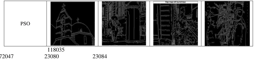
Image

Ground Truth

DPSO

CANNY

ACO

PSO

118035

372047

23080

23084

Fig. 3“Four example test images from the BSD500 dataset detected by DPSO (Distinct Particle Swarm Optimisation), Canny, ACO, GA and PSO edge detectors”

Image

Ground Truth

DPSO

CANNY

ACO

International Journal of Innovative Technology and Exploring Engineering (IJITEE) ISSN: 2278-3075, Volume-8 Issue-9, July 2019

PSO

288024 56028

12003 35010

Fig. 4“Four example test images from the BSD500 dataset detected by DPSO (Distinct Particle Swarm Optimisation), Canny, ACO, GA and PSO edge detectors

TABLE I

“Test Performance (F Score, Recall and Precision) for DPSO, Canny, ACO, GA and PSO Edge Techniques on First Four Images”

Image Techniq

ues

Precision Recall F Score

118035

DPSO 0.4289 0.4053 0.4168

PSO 0.3101 0.3140 0.3120

ACO 0.1892 0.1815 0.1853

GA 0.1452 0.1534 0.1482

Canny 0.1387 0.1254 0.1317

372047

DPSO _{0.3914 0.3874 0.3983}

PSO 0.2187 0.2215 0.2201

ACO 0.2110 0.2147 0.2129

GA 0.1874 0.1965 0.1918

Canny 0.1967 0.2018 0.1993

23080

DPSO 0.2542 0.2431 0.2486

PSO 0.1794 0.1685 0.1737

ACO 0.1301 0.1398 0.1347

GA 0.1123 0.1223 0.1171

Canny 0.1367 0.1272 0.1317

23084

DPSO 0.2916 0.2998 0.2957

PSO 0.2512 0.2547 0.2528

ACO 0.1587 0.1604 0.1596

GA 0.1498 0.1487 0.1492

Canny 0.1912 0.1877 0.1884

TABLE II

“Test Performance (F Score, Recall and Precision) for DPSO, Canny, ACO, GA and PSO Edge Techniques on Last Four Images”

Image Techniq

ues

Precision Recall F Score

288024

DPSO 0.3553 0.3413 0.3482

PSO 0.2865 0.2932 0.2898

ACO 0.2216 0.2361 0.2286

GA 0.2038 0.1932 0.1984

Canny 0.1587 0.1491 0.1538

56028

DPSO 0.3781 0.3863 0.3822

PSO 0.3067 0.2987 0.3026

ACO 0.2786 0.2697 0.2741

GA 0.2436 0.2503 0.2470

Canny 0.1865 0.1978 0.1919

DPSO 0.5324 0.5268 0.5296

PSO 0.3836 0.3798 0.3816

12003

ACO 0.3201 0.3147 0.3173

GA 0.2765 0.2675 0.2719

Canny 0.2065 0.1987 0.2025

35010

DPSO 0.4267 0.4186 0.4226

PSO 0.3742 0.3821 0.3781

ACO 0.2975 0.3012 0.2993

GA 0.2134 0.2236 0.2098

Canny 0.1567 0.1634 0.1599

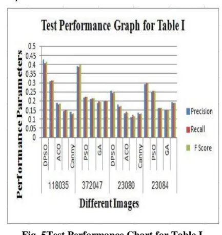
The test performance chart for table I shows in fig.5. From the graph we conclude that the Distinct particle Swarm Optimization (DPSO) techniques gives the best value of performance parameters as compared to the other techniques.

Fig. 6Test Performance Chart for Table II TABLE III

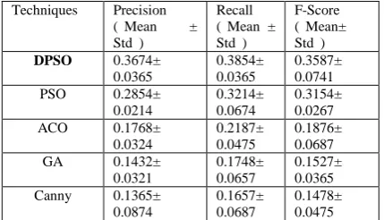
“Mean and standard deviation test result of all edge detectors on 100 test images from BSD500 dataset.”

Techniques Precision (“Mean ± Std”)

Recall (“Mean ± Std”)

F-Score (“Mean± Std”) DPSO 0.3674±

0.0365

0.3854± 0.0365

0.3587± 0.0741 PSO 0.2854±

0.0214

0.3214± 0.0674

0.3154± 0.0267 ACO 0.1768±

0.0324

0.2187± 0.0475

0.1876± 0.0687 GA 0.1432±

0.0321

0.1748± 0.0657

0.1527± 0.0365 Canny 0.1365±

0.0874

0.1657± 0.0687

0.1478± 0.0475

Mean and standard deviation of all approaches when tested on 100 BSD test images are shown in Table III. It is also clearly visible from Table III that DPSO also outperforms all other edge detection techniques when tested on 500 test images

V. CONCLUSION/FUTURE SCOPE

In this paper new objective function based “distinct particle swarm optimization (DPSO)” is proposed to identify unbroken edges in an image. “The new objective function achieves the goal by establishing the probability measure of the curve to be an edge. The proposed algorithm was tested and the results are compared with the different edge detection techniques such as Canny, ACO, GA and PSO on eight images which are taken from BSD500 dataset.” The new algorithm gives better result as compared to the other techniques.The processing time of Distinct Particle Swarm Optimization (DPSO)” algorithm is more as compared to canny operator.” Thus reducing the processing time of the technique is future study to the researchers. Be that as it may, the new edge detection algorithm gives the most astounding “Precision, Recall and F-Score” value as compared to the other edge detectors under all conditions. Experiment results of the images demonstrated that under all conditions, “DPSO” display better performance.

REFERENCES

1. J. Canny, “A computational approach to edge detection,” IEEE Trans. Pattern Anal. Mach. lntell. PAMI-8, pp. 679-698, 1986.

2. N. S. Dagar, P. K. Dahiya, “Soft Computing Techniques for Edge Detection Problem: A state-of-the-art Review”, International Journal of Computer Applications (0975 – 8887) Volume 136 – No.12, February 2016.

3. N. S. Dagar, P. K. Dahiya, “A Comparative Analysis of Edge Detection Algorithm and Performance Metric Using Precision, Recall

and F- Score”, International Journal of Modern Electronics and Communication Engineering (IJMECE) ISSN: 2321-2152 Volume No.-6, Issue No.-6, November, 2018.

4. S. M. Bhandarkar, Y. Zhang and W. D. Potter, “An edge detection technique using genetic algorithm-based optimization,” Pattern Recognition, vol. 27, pp. 1159–1180, 1994.

5. P. Arbelaez, M. Maire, C. Fowlkes and J. Malik, “Contour Detection and Hierarchical Image Segmentation”, IEEE Transactions on Pattern Analysis and Machine Intelligence, volume 33, issue-5, May 2011.

6. C. Bruni, A. De Santis, D. Iacoviello and G. Koch, “Modeling for edge detection problems in blurred noisy images,” IEEE Transactions on Image Processing, vol. 10, pp. 1447–1453, 2001.

7. E. Nadernejad, S. Sharifzadeh, H. Hassanpour, “Edge Detection Techniques: Evaluations and Comparisons,” Applied Mathematical Sciences, vol. 2, pp. 1507 – 1520, 2008.

8. Li Jing, Huang Peikang, Wang Xiaohu& Pan Xudong, “Image Edge Detection Based On Beamlet Transform,” Journal of Systems Engineering and Electronics, vol. 20, no. 1,pp. 1-5, 2009.

9. M.Setayesh, M. Zhang and M. Johnston, “Improving edge detection using particle swarm optimization”, in Proceeding of the 25th International conference on Image and Vision Computing, New Zealand, IEEE Press, 2010.

10. H. L. Tan, S. B. Gelfand and E. J. Delp,”A cost minimization approach to edge detection using simulated annealing,” IEEE Trans. Pattern Anal. Mach. Intell. Vol. 14, pp. 3-18, 1991.

11. J. Kennedy, R. Eberhart, “Particle swarm optimization,” in IEEE International Conference on Neural Networks, vol. 4,pp. 1942–1948, 1995.

12. S. L. Gupta, A. S. Baghel and A. Iqbal, "Threshold Controlled Binary Particle Swarm Optimization for High Dimensional Feature Selection", International Journal of Intelligent Systems and Applications(IJISA), Vol.10, No.8, pp.75-84, 2018.

13. M. Braik, A. Sheta and A. Ayesh, “Image Enhancement Using Particle Swarm Optimization,” Proceedings of the World Congress on Engineering, pp. 1-6, 2007.

14. D. Martin, C. Fowlkes, and J. Malik, “Learning to detect natural image boundaries using local brightness, color, and texture cues,” IEEE Trans. Pattern Anal. Mach. Intell., vol. 26, no. 5, pp. 530–549, May 2004.

15. M. Setayesh, M. Zhang and M. Johnston, ”Edge Detection Using Constrained Discrete Particle Swarm Optimization in Noisy Images”, IEEE 2011 Congress of Evolutionary Computation (CEC), page no.246-253.

AUTHOR’S PROFILES

Naveen Singh Dagar received his M.Tech (Electronics & Communication) from DeenbandhuChhotu Ram University of Science & Technology, Murthal, Sonepat, Haryana, India. Currently, he is research scholar at DeenbandhuChhotu Ram University of Science & Technology, Murthal, Sonepat, Haryana, India. His research includes Soft Computing Techniques for Edge Detection.