Impact of gravity wave drag on the thermospheric circulation: implementation of a nonlinear gravity wave parameterization in a whole atmosphere model

https://doi.org/10.5194/angeo-37-955-2019 © Author(s) 2019. This work is distributed under the Creative Commons Attribution 4.0 License.

Impact of gravity wave drag on the thermospheric circulation:

implementation of a nonlinear gravity wave parameterization

in a whole-atmosphere model

Yasunobu Miyoshi1and Erdal Yi˘git2

1_{Department of Earth and Planetary Sciences, Kyushu University, Fukuoka, Japan}

2_{Space Weather Laboratory, Department of Physics and Astronomy, George Mason University, Fairfax, VA, USA} Correspondence:Yasunobu Miyoshi (y.miyoshi.527@m.kyushu-u.ac.jp)

Received: 8 March 2019 – Discussion started: 25 March 2019

Revised: 5 August 2019 – Accepted: 19 September 2019 – Published: 17 October 2019

Abstract.To investigate the effects of the gravity wave (GW) drag on the general circulation in the thermosphere, a non-linear GW parameterization that estimates the GW drag in the atmosphere system is implemented in a whole-atmosphere general circulation model (GCM). Comparing the simulation results obtained with the whole-atmosphere scheme with the ones obtained with a conventional linear scheme, we study the GW effects on the thermospheric dy-namics for solstice conditions. The GW drag significantly decelerates the mean zonal wind in the thermosphere. The GWs attenuate the migrating semidiurnal solar-tide (SW2) amplitude in the lower thermosphere and modify the lati-tudinal structure of the SW2 above a 150 km height. The SW2 simulated by the GCM based on the nonlinear whole-atmosphere scheme agrees well with the observed SW2. The GW drag in the lower thermosphere has zonal wavenum-ber 2 and semidiurnal variation, while the GW drag above a 150 km height is enhanced in high latitude. The GW drag in the thermosphere is a significant dynamical factor and plays an important role in the momentum budget of the ther-mosphere. Therefore, a GW parameterization accounting for thermospheric processes is essential for coarse-grid whole-atmosphere GCMs in order to more realistically simulate the atmosphere–ionosphere system.

1 Introduction

are characteristic of the thermosphere–ionosphere system, as documented for the first time in the context of a parame-terization in the work by Yi˘git et al. (2008). These wave-damping mechanisms are molecular diffusion and thermal conduction and ion drag in addition to nonlinear interactions. Therefore, in order to realistically simulate GW dynamics in the thermosphere, these processes have to be taken into ac-count. The majority of the conventional GW schemes were not designed for the upper atmosphere in the first place.

Recently, an increasing number of numerical studies have revealed direct upward propagation of GWs from the lower atmosphere into the thermosphere and demonstrated sig-nificant GW effects on the thermospheric circulation (e.g., Yi˘git et al., 2014; Heale et al., 2014; Gavrilov and Kshevet-skii, 2015). Earlier, using a regional model and ray-tracing method, Vadas and Fritts (2004) showed that GWs generated by cumulus convection can propagate into the thermosphere and produce large GW drag in the thermosphere. GWs with high frequency (large vertical wavelength) can penetrate into the thermosphere (Vadas and Fritts, 2005). Yi˘git et al. (2008) developed a nonlinear whole-atmosphere GW parameteriza-tion and succeeded in the implementaparameteriza-tion and applicaparameteriza-tion of their GW parameterization in the Coupled Middle Atmo-sphere ThermoAtmo-sphere-2 (CMAT2) general circulation model (GCM). Yi˘git et al. (2009) showed that the dynamical effects of gravity waves in the thermosphere are comparable with the ion-drag effects up to ionospheric F2-region altitudes. Later, based on the similar modeling framework, Yi˘git and Medvedev (2009) showed for the first time that GW thermal effects are very important globally in the thermosphere, com-peting with joule heating, and ultimately cool the thermo-sphere. More recently, Yi˘git and Medvedev (2017) demon-strated that the small-scale GWs impact the amplitude of the diurnal tide in the low-latitude middle atmosphere and in the high-latitude thermosphere. Using the first-generation CMAT model with two different older GW parameteriza-tions, England et al. (2006) investigated effects of the GW drag on the diurnal tide and green-line airglow emissions during equinox in the equatorial mesosphere and lower ther-mosphere (MLT). Based on idealized numerical simulations with the Yi˘git et al. (2008) scheme, Medvedev et al. (2017) have discovered that the magnetic field configuration can sig-nificantly influence the propagation and dissipation of lower-atmospheric GWs in the thermosphere via the ion-drag force. GW effects can also be studied using high-resolution GCMs. Models are increasingly capable of implement-ing higher resolutions, which can capture smaller-scale physics. Using a GW-resolving (i.e., high horizontal reso-lution) GCM, Miyoshi and Fujiwara (2008) and Miyoshi et al. (2014, 2015) investigated upward propagation of GWs and the GW drag in the thermosphere. They indicated that the GW drag in the thermosphere is much larger than that in the mesopause region. The GW activity in the thermosphere is stronger in winter than in summer and is correlated with the strength of the strato-mesospheric jet. Using a GW-resolving

Whole Atmosphere Community Climate Model (WACCM), Liu et al. (2014) also studied upward propagation of GWs excited by tropical convection up to a 105 km height. Over-all, high-resolution simulations supported the finding that the mean GW effects in the thermosphere can be adequately rep-resented by physics-based GW parameterizations, such as the one developed in the work by Yi˘git et al. (2008).

Previous numerical studies indicated that the GW drag plays an important role in maintaining the momentum and energy balance in the thermosphere. Both GW parameteri-zations and high-resolution simulations provide various ad-vantages as well as some limitations. While the mean global structure of GW effects is well represented by GW parame-terizations extending into the thermosphere, high-resolution simulations can more self-consistently simulate GW pro-cesses probably in more detail; for example, smaller-scale variability in GWs can be better captured. This implies over-all that a GW-resolving GCM is necessary in order to simu-late thermospheric circulation more accurately. However, nu-merical diffusion schemes (e.g., hyperdiffusivity) may exces-sively damp smaller-scale GWs. Often, GW sources and their generations are still parameterized in high-resolution simula-tions. Also, conducting numerical simulations with a GW-resolving GCM requires high-performance computer sys-tems and overall needs much more computational time and data storage. Therefore, long-term simulations using a GW-resolving GCM are unpractical. Therefore, a low-resolution GCM based on a physics-based whole-atmosphere GW pa-rameterization is strongly required. However, there are only a few studies concerning GW drag parameterization for the thermosphere, and there are various aspects of GW effects in the thermosphere that are still unexplored. One such unex-plored territory that is the focus of this paper is the interaction of GWs with the semidiurnal migrating tide (SW2) in the up-per atmosphere. Simultaneously, this work serves as the first study with the whole-atmosphere GCM by Miyoshi and Fu-jiwara (2003) implementing the whole-atmosphere GW pa-rameterization by Yi˘git et al. (2008). Thus, we will also study and revisit the mean GW effects on the thermosphere and so-lar tides.

The descriptions of the GCM, the GW parameterization, and numerical simulations are presented in Sect. 2. Results and discussions are presented in Sect. 3. Concluding remarks follow in Sect. 4.

2 General circulation model, gravity wave schemes, and experiment design

lati-tude×2.8◦longitude. The GCM has 150 layers, with a ver-tical resolution of 0.2-scale heights. The GCM covers the re-gion from the ground to the exobase. It has a complete set of physical processes appropriate for the whole-atmosphere re-gion. The GCM is the same as the neutral atmospheric part of an atmosphere–ionosphere coupled model, GAIA (Ground-to-topside model of Atmosphere and Ionosphere for Aeron-omy; Jin et al., 2008, 2012).

The GCM incorporates schemes for a hydrological cycle, a boundary layer, moist convection, and infrared and solar radiations (Miyoshi and Fujiwara, 2003; Miyoshi, 2006). Ef-fects of mountains and land–sea contrast are also taken into account. The GCM was nudged by Japanese Meteorological Agency reanalysis data (JRA-55; Kobayashi et al., 2015) up to a 40 km height to simulate realistic temporal variations in the lower atmosphere (Jin et al., 2012). In the thermosphere, the GCM has schemes for molecular diffusion, thermal con-ductivity, joule heating, ion-drag force, and auroral precip-itation heating. To estimate joule heating, ion-drag force, and auroral precipitation heating, the electron density is pre-scribed using an empirical ionosphere model. The global electron density distribution produced by the solar radiation is represented by Chiu’s empirical model (Chiu, 1975). Elec-trons produced by auroral particles are estimated by Fuller-Rowell and Evans (1987). We use a coarse grid in this study, which provides computational efficiency, and represent GWs that are not explicitly resolved by the model with orographic and nonorographic GW parameterizations. The GW parame-terization developed by McFarlane (1987) is used for oro-graphic GWs. The previous standard version of the GCM includes a linear nonorographic GW parameterization devel-oped by Lindzen (1981). However, the GW drag estimated by these GW parameterizations is taken into account only below a 100 km height. Thus, note that no GW effects are calculated in the thermosphere above a 100 km height in this configura-tion. This setup mimics the traditional approach of account-ing for GWs only in the middle atmosphere, which is essen-tially what low-top middle-atmosphere models used to do. The numerical simulation using this original GCM is called EXP1. This standard version is described in detail in previous publications (Miyoshi and Fujiwara, 2003; Miyoshi, 2006; Miyoshi et al., 2009).

To assess impacts of GW drag on the general circulation in the thermosphere as well as in the lower and middle at-mosphere, we need a GW scheme that extends into the ther-mosphere. Therefore, the GW parameterization developed in the work by Yi˘git et al. (2008) has been implemented in the GCM developed by Miyoshi and Fujiwara (2003). Yi˘git’s GW parameterization can estimate the GW effects in the whole-atmosphere system from the troposphere to the up-per thermosphere. The GW spectrum is specified in terms of momentum fluxes as a function of horizontal phase speeds. The phase speeds of GWs used in GW calculations range from 2 to 80 m s−1. The peak GW flux at the source level and the horizontal wavenumber are set at 0.00025 m2s−2

and 2π/250 km−1, respectively (see Fig. 1 of Yi˘git et al., 2012, for a representative GW spectrum). The GW spec-trum adopted in this study and its relation to the observation were discussed in detail in Yi˘git et al. (2008). Dissipation of gravity waves due to nonlinear interactions (Medvedev and Klaassen, 2000), radiative damping, molecular diffusion and thermal conduction, eddy viscosity, and ion drag are taken into account. This scheme has been used successfully in dif-ferent Earth-modeling frameworks (e.g., Lübken et al., 2018) and also for Mars’ atmosphere (Yi˘git et al., 2018). The nu-merical simulation with Yi˘git’s whole-atmosphere parame-terization is called EXP2. The GCM used in EXP1 is identi-cal to the GCM used in EXP2 except for the nonorographic GW parameterization. Namely, in EXP2, Lindzen’s GW pa-rameterization, which cuts off GW effects at around 100 km, is replaced by Yi˘git’s GW parameterization, which calculates GW effects in the entire atmosphere. By comparing EXP1 and EXP2, we investigate the impact of the GW drag on the general circulation in the middle and upper atmospheres by comparing EXP1 and EXP2.

To exclude influences from temporal variations in solar UV and EUV fluxes and geomagnetic activity, we performed the numerical simulations under solar minimum and geo-magnetically quiet conditions. The 10.7 cm solar radio flux (F10.7) was fixed at 70×10−22W m−2Hz−1, and the cross-polar potential was set at 30 kV during the numerical sim-ulations. Numerical simulations were conducted under June solstice conditions. Numerical simulation started on 1 June (year 2015), and a 2-year numerical integration with seasonal variation was performed. The time step of the GCM is 30 s, and the GW drag is estimated at each time step. The data are sampled every 1 h during the numerical simulation. The data from 1 to 30 June in the second year (year 2016) are analyzed in this study.

3 Results and discussions 3.1 Zonal-mean fields

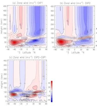
is located at 50◦N, whereas the peak of the eastward wind (20–25 m s−1_{) above a 120 km height appears at 30}◦_S.

Figure 1b shows the zonal and diurnal-mean zonal-wind distribution obtained by the application of the Yi˘git scheme (EXP2). As shown before, Yi˘git’s GW parameterization is implemented in the whole-atmosphere region. The strato-mesospheric jets weaken in the upper mesosphere, and the reversal of the zonal-wind direction occurs at a 80–100 km height. The difference of the zonal-mean zonal wind between EXP2 and EXP1 is shown in Fig. 1c. There are substan-tial differences of the magnitudes of the strato-mesospheric jets between EXP1 and EXP2. The eastward jet in the SH is stronger in EXP1 than in EXP2. On the other hand, the westward jet in the NH at 20–50◦N is stronger in EXP1 than in EXP2 by ∼22 m s−1, and the westward jet poleward of 50◦N is weaker in EXP1 than in EXP2 by∼8 m s−1. These differences of the strength of the jets are mainly caused by the differences of the GW drag distributions, as shown later (Sect. 3.4). Above a 120 km height, the westward and east-ward winds are dominant in the NH and SH, respectively. These features obtained in EXP2 are the same as those in EXP1. However, the reversal of the zonal-wind direction at a 80–100 km height is much clearer in EXP2 than in EXP1. The peak values of the zonal-mean zonal wind above a 120 km height are weaker in EXP2 than in EXP1. These results indicate that including GW effects above a 100 km height affects the magnitude of the zonal-mean zonal wind and provides a deceleration mechanism.

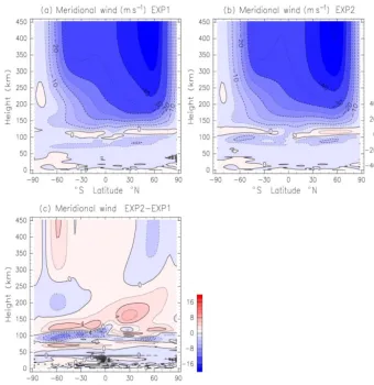
Figure 2a and b show the height–latitude distribution of the zonal-mean meridional wind obtained by EXP1 and EXP2, respectively. In both experiments, southward flow from the summer pole to winter pole is dominant at a 50–100 km height, whereas northward flow appears between a 100 and 120 km height. These flows are stronger in EXP2 than in EXP1, which is explained by the enhanced GW drag in EXP2 as shown later. Above a 130 km height, southward flow is dominant in both experiments. The magnitude of the southward wind between a 130 and 250 km height is weaker in EXP2 than that in EXP1 except for southward of 30◦S (Fig. 3c). This weaker meridional wind in EXP2 is caused by the meridional component of the GW drag. On the other hand, the difference of meridional wind between EXP1 and EXP2 is small above a 250 km height (less than 10 %).

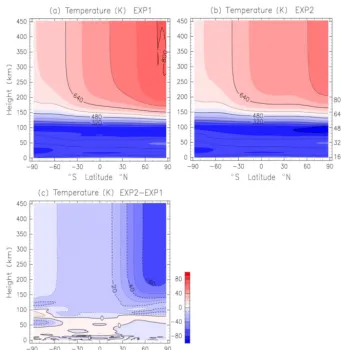
Figure 3a and b show the height–latitude distribution of the zonal-mean temperature obtained by EXP1 and EXP2, respectively. At a 80–100 km height, Cooling and warming occur at 30–90◦_{N and at 60–90}◦_{S, respectively (Fig. 3c).}

This cooling and warming is caused by the enhanced south-ward wind (meridional circulation) at a 80–100 km height in EXP2. Namely, the cooling (warming) at 30–90◦N (60– 90◦S) is due to enhanced upward (downward) wind. It is noteworthy that cooling prevails above a 100 km height. In particular, cooling at high latitudes in the NH exceeds 60 K. This cooling is caused by the GW thermal effect. This indi-cates that GW-induced cooling also affects thermal structure

in the upper thermosphere. Our results support the conclu-sion of the GCM work by Yi˘git and Medvedev (2013), who showed for the first time that GWs cool the thermosphere during low solar-activity conditions.

3.2 Migrating semidiurnal tide

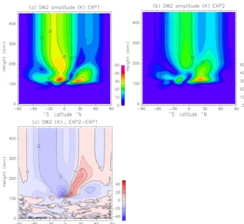
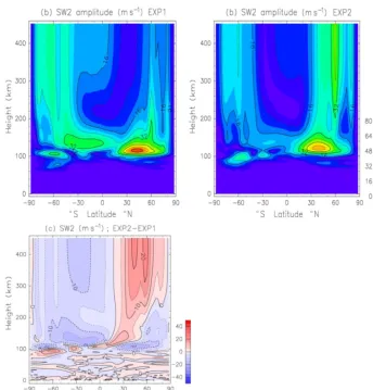
The impact on the migrating semidiurnal tide (SW2) is ex-amined here. Figure 4a shows the height–latitude distribu-tion of the temperature component of the SW2 amplitude in June obtained by EXP1. The amplitude maximizes at around a 125 km height. The maxima are 41 K at 15◦S and 38 K at 20◦N. The peak of the SW2 amplitude above a 200 km height (34 K) appears at 15–25◦S, and the secondary peak (10 K) is found around 45◦N. Using the SABER (Sounding of the Atmosphere using Broadband Emission Radiometry) measurement aboard the TIMED (Thermosphere Ionosphere Mesosphere Energetics Dynamics) satellite, Pancheva and Mukhtarov (2011) studied climatology (6-year mean from 2002 to 2007) of SW2 temperature tide observation. Fig-ure 2.3 in Pancheva and Mukhtarov (2011) indicates that the SW2 in June at a 110 km height has peaks at 15–30◦N and 15–25◦S. The maxima at 15–30◦N and at 15–25◦S are 25–28 and 15–20 K, respectively. The peak values at a 110 km height in EXP1 are about 30–35 K, which is much larger than the observation. Forbes et al. (2011) investigated seasonal variation in the SW2 in the exobase (about 400– 500 km) using the CHAMP (CHAllenging Minisatellite Pay-load) and GRACE (Gravity Recovery and Climate Experi-ment) accelerometer measurements. The observed SW2 in June also has two peaks (15–20◦S and 40◦N), and the peak value during the solar minimum is 24 K (Figs. 7 and 8 of Forbes et al., 2011). The simulated SW2 in the SH (NH) is larger (smaller) than the observed SW2.

Figure 4b shows the temperature component of the SW2 amplitude obtained by EXP2. The SW2 in the lower thermo-sphere maximizes at 15–20◦S and at 20◦N. The peak values of the monthly mean SW2 amplitude in EXP2 at a 110 km height are 26 K at 20◦N and 21 K at 15◦S. The SW2 peaks at a 100–200 km height move southward in EXP2. The SW2 amplitude in the lower thermosphere in EXP2 is weaker than the one in EXP1 by about 20 %–40 % (Fig. 4c). Results ob-tained with EXP2 compare better with the observed SW2 amplitude. Above a 200 km height, the SW2 amplitude in EXP2 maximizes at 10◦S (25 K), and the secondary peak is found at 40◦N (15–20 K). The SW2 amplitude in the SH (NH) is weaker (stronger) in EXP2 than in EXP1. This means that the latitudinal structure of the SW2 above a 200 km height is modified by GW propagating and dissipation in the middle and upper thermosphere. Moreover, the SW2 in the upper thermosphere obtained by EXP2 agrees well with the observed SW2 amplitude.

Figure 1. (a)Height–latitude section of zonal and diurnal-mean zonal wind obtained by EXP1 (the application of the Lindzen scheme below 100 km height). Data are averaged from 1 to 30 June. Contour intervals of black lines are 10 m s−1. Negative and positive values are eastward and westward winds, respectively.(b)As in(a)except for the application of the Yi˘git scheme in the whole atmosphere (EXP2).(c)Difference of the zonal wind between EXP1 and EXP2 (EXP2–EXP1). Contour intervals are 5 m s−1.

The maximum of the zonal-wind component of the SW2 at a 120 km height in EXP1 (EXP2) is 68 m s−1 (55 m s−1). The GW parameterization attenuates the zonal-wind com-ponent of the SW2 in the lower thermosphere. Moreover, above a 200 km height, the GW parameterization modifies the latitudinal structure of the zonal-wind component. The effects of the GW drag on the migrating diurnal tide in the MLT was studied by Miyahara and Forbes (1991). They showed that the DW1 is attenuated by the GW drag. Yi˘git and Medvedev (2017) investigated the effects of GWs on the diurnal tide from the mesosphere to the upper thermosphere. They found that while GWs enhance the tidal amplitude in the MLT, GWs can both damp and strengthen the tides in the thermosphere. The impact on DW1 obtained in this study is similar to that in Yi˘git and Medvedev. On the other hand, the present results indicate that the GW drag has wide-reaching implications for the migrating tides. Namely GWs attenuate the SW2 amplitude in the MLT, improving model

simula-tions with respect to observasimula-tions. Overall, this is the most dominant effect of the GW drag on the SW2.

The SW2 also has significant day-to-day variations. For example, the SW2 amplitude at 20◦N in EXP1 ranges from 27 to 37 K, whereas the SW2 amplitude in EXP2 ranges from 22 to 31 K. The standard deviation of day-to-day variations in the SW2 amplitude at 20◦N in EXP1 and EXP2 is 2.8 and 2.9 K, respectively. Similar day-to-day variations in the SW2 amplitude are found below a 100 km height. These results indicate that day-to-day variations in the SW2 amplitude are primarily generated in the lower atmosphere and propagate into the lower thermosphere.

3.3 Migrating terdiurnal tide

Figure 2. (a)Zonal-mean meridional wind obtained by EXP1 (Lindzen’s parameterization below 100 km height). Data are averaged from 1 to 30 June. Negative and positive values are southward and northward wind, respectively. Contour intervals are 5 m s−1.(b)As in(a)except for EXP2 (Yi˘git’s parameterization in the whole atmosphere).(c)Meridional wind difference between EXP1 and EXP2 (EXP2–EXP1). Contour intervals are 2 m s−1.

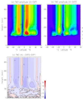
located at 15◦N latitude, and the secondary peak appears at 25–30◦S. The maxima are 23 K at 15◦N and a 130 km height and 18 K at 17.5◦S and a 165 km height. Figure 6b shows the temperature component of the TW3 amplitude obtained by EXP2, and Fig. 6c shows the amplitude difference be-tween EXP1 and EXP2. The latitudinal structure of the TW3 in EXP2 is quite similar to that in EXP1. However, the ampli-tude is weaker in EXP2 than in EXP1 by about 20 %–40 %. The amplitude difference is significant in the 120–220 km height range. The TW3 is also attenuated by the GW drag. Forbes et al. (2008) indicated that the TW3 amplitude at a 110 km height is between 5 and 8 K. However, there are few studies concerning the satellite observation of TW3 ampli-tude in the 120–220 km height range. A detailed comparison of the TW3 amplitude between the simulation and observa-tion is a subject of a future study.

3.4 Zonal mean of the zonal GW drag

Figure 3. (a)Zonal-mean temperature obtained by EXP1 (Lindzen’s parameterization below 100 km height). Data are averaged from 1 to 30 June. Units are kelvins.(b)As in(a)except for EXP2 (Yi˘git’s parameterization in the whole atmosphere).(c)Temperature difference between EXP1 and EXP2 (EXP2–EXP1). Contour intervals are 10 K.

3.5 Longitudinal variation in the GW drag at 35◦_N

In the previous sections, we investigate zonal and diurnal mean of the GW drag. Longitudinal and diurnal variabilities in the winds are significant in the thermosphere, so longi-tudinal and diurnal variability of the GW drag is examined next. Figure 8a shows the height–longitude distribution of the zonal GW drag at 35◦N, where the SW2 amplitude max-imizes in the lower thermosphere. The zonal GW drag in Fig. 8a is averaged between 00:00 and 01:00 UT. The GW drag at a 70–100 km height is eastward at all longitudes and contributes the attenuation and reversal of the westward jet in the upper mesosphere.

The zonal and diurnal mean of the zonal GW drag at 35◦N in the 100–200 km height region is smaller than 20 m s−1d−1 (Fig. 7b). However, Fig. 8a indicates that the GW drag can range from−100 to 200 m s−1d−1within the 1 d period. The maximum acceleration is located at 157◦E and a 150 km height. The GW drag has a zonal wavenumber 2 structure in the 100–200 km height region, and the peak of the GW

drag descends with increasing longitude. Figure 8b shows a height–longitude section of the zonal wind at 35◦N averaged between 00:00 and 01:00 UT. The zonal-wind distribution in the 100–200 km height region has also zonal wavenumber 2 structure and descends with increasing longitude, indicat-ing characteristics of the upward-propagatindicat-ing SW2. The east-ward (westeast-ward) acceleration of GW drag in the 100–200 km region occurs in the region of westward (eastward) wind. It is clearly seen that the GW drag attenuates the zonal-wind variation associated with the SW2. Thus, the attenuation of the SW2 in EXP2 is explained by dissipating GWs as rep-resented by the Yi˘git scheme. The main dissipation mech-anisms of GWs in the thermosphere are due to ion drag, molecular diffusion, and thermal conduction, while in the MLT nonlinear interactions play an important role.

Figure 4. (a)Height–latitude distribution of the temperature component of the SW2 amplitude in June obtained by EXP1. Units are kelvins. Contour intervals are 5 K.(b)As in(a)except for EXP2.(c)Temperature difference between EXP1 and EXP2 (EXP2–EXP1).

The distribution of GW drag in 00:00–01:00 UT is clearly out of phase with that in 06:00–07:00 UT, indicating semid-iurnal variation in the GW drag. In the work by Miyoshi et al. (2014), the relationship between GW drag and SW2 was investigated using a GW-resolving GCM. They showed that the semidiurnal variation in the GW drag is significant in the lower thermosphere, and it decelerates the background zonal-wind variation. The present result is consistent with the result obtained by Miyoshi et al. (2014).

3.6 Longitudinal variation in the GW drag at high latitudes

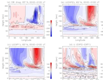
In this section, the relationship between the GW drag and the zonal wind in high latitudes, where the diurnal variation of the zonal wind is the largest, is investigated. Figure 10a shows the height–longitude section of the zonal GW drag in EXP2 at 65◦N in 00:00–01:00 UT. Eastward acceleration is dominant in the 60–110 km height region, which attenuates the westward wind. Above a 150 km height, zonal wavenum-ber 1 structure is dominant. Eastward acceleration (westward acceleration) appears in the 0–180◦E (180–360◦E) longi-tude sector. Studying the GW drag together with the zonal-wind (EXP2) distribution shown in Fig. 10b shows that the

GW drag is predominantly directed against the zonal wind and thus tends to decelerate the wind. It is noteworthy that the magnitude of eastward acceleration at a 130–270 km height is a few hundred meters per second per day, and the max-imum values of −650 m s−1d−1 is found at 275◦E and a 230 km height.

differ-Figure 5. (a)Height–latitude distribution of the zonal-wind component of the SW2 amplitude in June obtained by EXP1. Units are meters per second.(b)As in(a)except for EXP2.(c)Zonal-wind difference between EXP1 and EXP2 (EXP2–EXP1).

ences of the treatment of the GW process. These differences will be discussed in Sect. 3.7.

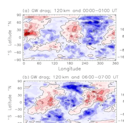
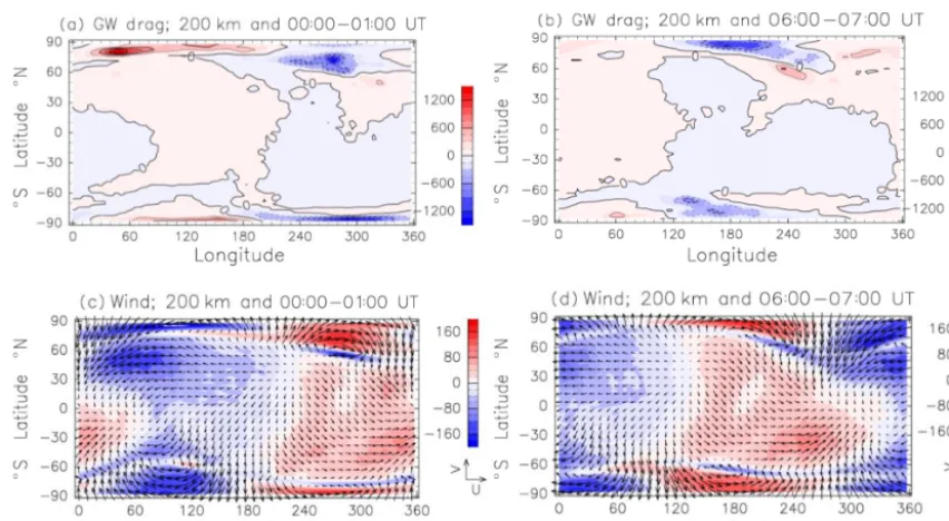
The global distribution of the zonal GW drag at a 200 km height is examined here. Figure 11a and b show the zonal GW drag distribution in 00:00–01:00 and 06:00–07:00 UT, respectively. In both figures, the GW drag is significant at high latitudes. For example, in 00:00–01:00 UT, westward acceleration of 1500 m s−1d−1 is found at 40–50◦E and 80◦N, while eastward acceleration of −1200 m s−1d−1 ap-pears at 275◦_{E and 70}◦_{N. These strong GW drag regions}

move westward with time, and westward acceleration of −1200 m s−1d−1 appears at 170◦E and 80◦N in 06:00– 07:00 UT. The magnitude of the GW drag in high latitudes is comparable to the magnitude of the ion-drag force (e.g., Yi˘git et al., 2012; Miyoshi et al., 2014).

Figure 11c and d show the horizontal wind distribution at a 200 km height in 00:00–01:00 and 06:00–07:00 UT, respec-tively. Colored shading in Fig. 11a and b shows the zonal-wind distribution. The enhanced zonal GW drag is located at the regions where the strong zonal wind appears. The

Figure 6. (a)Temperature component of the TW3 amplitude in June obtained by EXP1. Units are kelvins. Contour intervals are 5 K.(b)As in(a)except for EXP2.(c)Temperature difference between EXP1 and EXP2 (EXP2–EXP1). Contour intervals are 2.5 K.

3.7 Discussions

General circulation models (GCMs) provide a powerful methodology for studying the global effects of gravity waves (GWs) in the atmosphere. One strength is the continuous coverage of atmospheric layers; thus interaction processes between different layers can be studied. However, they have limited resolutions, so physical parameterizations are crucial. Nowadays, atmospheric models are gradually being con-verted into whole-atmosphere models, which can provide a framework in which atmospheric wave propagation can be studied from the lower atmosphere to the upper atmo-sphere in a more self-consistent manner (e.g., Miyoshi and Fujiwara, 2003, 2008; Akmaev et al., 2008). Also, it is in-creasingly acknowledged that GW parameterizations must

Figure 7. (a)Height–latitude section of the zonal mean of the zonal GW drag in June obtained by EXP1. Positive and negative values are eastward and westward acceleration, respectively. Units are me-ters per second per day.(b)As in(a)except for EXP2.

(Walterscheid and Hickey, 2012). Transient atmospheric pro-cesses can dramatically modulate penetration of GWs into the thermosphere. During minor warming, thermospheric GW activity can be enhanced significantly (e.g., Yi˘git et al., 2014; Yi˘git and Medvedev, 2016), while during major warm-ings it may encounter a decrease (Nayak and Yi˘git, 2019). Here, we used a whole-atmosphere GCM incorporating a whole-atmosphere GW parameterization in order to the study the mean dynamical effects of GWs and their impact on the semidiurnal tides in the thermosphere.

Using the SABER measurement aboard the TIMED satel-lite, Pancheva and Mukhtarov (2011) investigated the behav-ior of the SW2 in the MLT. There, the typical observed peak values for the SW2 amplitudes are situated at low latitudes during the June solstice: 25–28 K at 15–30◦_{N and 15–20 K}

at 15–25◦S. In our study, GCM simulations based on two different GW parameterizations yield different results for the SW2 tide. While the simulation with the standard Lindzen scheme overestimate the tidal amplitude, the one with the Yi˘git scheme matches observations better. This can be ex-plained by the additional GW drag in the thermosphere (i.e., additional physics) as accounted for by the Yi˘git scheme,

Figure 8. (a)Height–longitude section of the zonal GW drag at 35◦N obtained by EXP2. Data are averaged between 00:00 and 01:00 UT in June. Units are meters per second per day.(b)As in(a)

except for zonal-wind component. Units are meters per second.

Figure 10. (a)Height–longitude section of the zonal GW drag at 65◦N in June (EXP2). Data are averaged between 00:00 and 01:00 UT. Units are meters per second per day. Contour intervals are 50 m s−1d−1.(b)As in(a)except for zonal-wind component obtained by EXP2. Units are meters per second.(c)As in(b)except for EXP1.(d)Difference of the zonal wind at 65◦N between EXP1 and EXP2 (EXP2–EXP1). Units are meters per second. Contour intervals are 10 m s−1.

which attenuates the zonal-wind variation associated with the SW2.

Using the CHAMP and GRACE accelerometer measure-ments, Forbes et al. (2011) showed the SW2 amplitude in the upper thermosphere. The GCM without GW drag parameter-ization in the thermosphere fails to reproduce the observed SW2 in the upper thermosphere, whereas the GCM with the GW parameterization succeeds in reproducing the behavior of the observed SW2 in the upper thermosphere. This result also indicates the importance of the GW effects in the ther-mosphere.

There are substantial differences between the linear and the nonlinear schemes in the treatment of GW processes, as has been initially discussed in detail in the work by Yi˘git et al. (2008). One major difference is that the linear scheme is based on the linear saturation principle, ignoring wave–wave interactions, while the Yi˘git scheme takes into account not only nonlinear wave–wave interactions but also dissipation of GWs due to additional processes, such as ion drag, molec-ular viscosity, and thermal conduction, which are important dissipative processes in the thermosphere–ionosphere sys-tem. Any GCM that extends into the thermosphere, includ-ing a GW parameterization, must incorporate these effects on GW propagation. While the linear scheme assumes an ar-tificial tuning factor for the GW drag, the nonlinear scheme does not require any artificial tuning parameters. However,

GW parameterizations are not devoid of limitations. They all assume a single-column approach and instantaneous re-sponse of the flow field to the upward-propagating waves.

The whole-atmosphere GCM uses an empirical spheric model. At high latitudes, the behavior of the iono-sphere can substantially influence the thermospheric circu-lation. On the other hand, the background atmosphere is very important for the GW propagation and dissipation. A modeling framework with a self-consistent two-way coupled ionosphere–thermosphere system could provide a more real-istic picture of ion-neutral coupling, and GW effects could be evaluated more precisely at high latitudes.

4 Concluding remarks

The GW parameterization developed by Yi˘git et al. (2008) has been implemented in the Japanese Kyushu University whole-atmosphere GCM (Miyoshi and Fujiwara, 2008), and the impact of small-scale GWs on the migrating semidiurnal tide as well as the GW effects on the general circulation of the thermosphere have been studied. We obtained the follow-ing results.

Figure 11. (a)Longitude–latitude section of the zonal GW drag at 200 km height in June. Data are averaged between 00:00 and 01:00 UT. Positive and negative values are eastward and westward acceleration, respectively. Units are meters per second per day. Contour intervals are 200 m s−1d−1.(b)As in(a)except for the average between 06:00 and 07:00 UT.(c)Vectors indicate the global distribution of the horizontal wind at 200 km height obtained by EXP2. Data are averaged between 00:00 and 01:00 UT in June. The vectors on the right-hand side indicate the zonal wind and meridional winds with magnitudes of 200 m s−1. Color bars are the global distribution of the zonal-wind component at 200 km height. Data are averaged between 00:00 and 01:00 UT.(d)As in(c)except for the average between 06:00 and 07:00 UT.

The GW drag modifies the zonal-mean meridional and temperature distributions in the thermosphere.

2. The GW drag attenuates the SW2 amplitude in the lower thermosphere and modifies the latitudinal structure of the SW2 above a 150 km height. The GW drag also at-tenuates the TW3 amplitude in the thermosphere.

3. The GW drag in the lower thermosphere has zonal wavenumber 2 structure and has semidiurnal variation.

4. The GW drag above a 150 km height is enhanced in high latitudes. The maximum value sometimes exceeds 1000 m s−1d−1. This means that the GW drag plays an important role in the momentum balance in high lati-tudes above a 150 km height.

The whole-atmosphere GCM used in this study uses an em-pirical ionosphere. Therefore, impacts of the GW drag on the ionospheric variability have not been investigated in this study. In the next step, implementation of GW drag parame-terization in an atmosphere–ionosphere coupled model, such as GAIA (Jin et al., 2012), is strongly required. Using an atmosphere–ionosphere coupled model with GW drag, we will investigate impacts of the GW drag on the ionospheric variability.

Data availability. Upon request, the data used for the pub-lication of this study are available from Yasunobu Miyoshi (y.miyoshi.527@m.kyushu-u.ac.jp).

Author contributions. YM performed the simulation and wrote a substantial portion of the paper. EY provided the whole-atmosphere GW parameterization scheme and significantly contributed to writ-ing and discussion of results.

Competing interests. Erdal Yi˘git is one of the editors of this special issue. The authors declare that they have no conflict of interest.

Special issue statement. This article is part of the special issue “Vertical coupling in the atmosphere–ionosphere system”. It is a result of the 7th Vertical coupling workshop, Potsdam, Germany, 2–6 July 2018.

Financial support. This research has been supported by the JSPS, Japan (grant no. 15H03733); the JSPS, Japan (grant no. 18H04447); and the National Science Foundation, USA (grant no. AGS 1452137).

Review statement. This paper was edited by Kathrin Baumgarten and reviewed by two anonymous referees.

References

Akmaev, R. A., Fuller-Rowell, T. J., Wu, F., Forbes, J. M., Zhang, X., Anghel, A. F., Iredell, M. D., Moorthi, S., and Juang, H.-M.: Tidal variability in the lower thermosphere: Compar-ison of Whole Atmosphere Model (WAM) simulations with observations from TIMED, Geophys. Res. Lett., 35, L03810, https://doi.org/10.1029/2007GL032584, 2008.

Chiu, Y. T.: An improved phenomenological model of ionospheric density, J. Atmos. Terr. Phys., 37, 1563–1570, 1975.

England, S. L., Dobbin, A., Harris, M. J., Arnold, N. F., and Aylward, A. D.: A study into the effects of gravity wave ac-tivity on the diurnal tide and airglow emissions in the equa-torial mesosphere and lower thermosphere using the Cou-pled Middle Atmosphere and Thermosphere (CMAT) general circulation model, J. Atmos. Sol.-Terr. Phy., 68, 293–308, https://doi.org/10.1016/j.jastp.2005.05.006, 2006.

Forbes, J. M., Zhang, X., Palo, J., Russell, C., Mertens, J., and Mlynczak M.: Tidal variability in the iono-spheric dynamo region, J. Geophys. Res., 113, A02310, https://doi.org/10.1029/2007JA012737, 2008.

Forbes, J. M., Zhang, X., Bruinsma, S., and Oberheide, J.: Sun-synchronous thermal tides in exosphere temperature from CHAMP and GRACE accelerometer measurements, J. Geophys. Res., 116, A11309, https://doi.org/10.1029/2011JA016855, 2011.

Fuller-Rowell, T. J. and Evans D. S.: Height-integrated Pedersen and Hall conductivity patterns inferred from the TIROS-NOAA satellite data, J. Geophys. Res., 92, 7606–7618, 1987.

Garcia, R. and Solomon, S.: The effect of breaking gravity waves on the dynamics and chemical composition of the mesosphere and lower thermosphere, J. Geophys. Res., 90, 3850–3868, 1985. Gavrilov, N. M. and Kshevetskii S. P.: Dynamical and thermal

ef-fects of nonsteady nonlinear acoustic-gravity waves propagating from tropospheric sources to the upper atmosphere, Adv. Space Res., 56, 1833–1843, 2015.

Heale, C. J., Snively, J. B., Hickey, M. P., and Ali, C. J.: Thermospheric dissipation of upward propagating grav-ity wave packets, J. Geophys. Res., 119, 3857–3872, https://doi.org/10.1002/2013JA019387, 2014.

Hickey, M. P., Walterscheid, R. L., and Schubert, G.: Gravity wave heating and cooling of the thermosphere: Sensible heat flux and viscous flux of kinetic energy, J. Geophys. Res., 116, A12326, https://doi.org/10.1029/2011JA016792, 2011.

Jin, H., Miyoshi, Y., Fujiwara, H., and Shinagawa, H.: Elec-trodynamics of the formation of ionospheric wave number 4 longitudinal structure, J. Geophys. Res., 113, A09307, https://doi.org/10.1029/2008JA013301, 2008.

Jin, H., Miyoshi, Y., Pancheva, D., Mukhtarov, P., Fujiwara, H., and Shinagawa, H.: Response of migrating tides to the stratospheric sudden warming in 2009 and their effects on the ionosphere stud-ied by a whole atmosphere-ionosphere model GAIA with COS-MIC and TIMED/SABER observations, J. Geophys. Res., 117, A10323, https://doi.org/10.1029/2012JA017650, 2012.

Kobayashi, S., Ota, Y., Harada, Y., Ebita, A, Moriya, M., Onoda, H., Onogi, K., Kamahori, H., Kobayashi, C., Endo, H., Miyaoka, K., and Takahashi, K.: The JRA-55 Reanalysis, J. Meteorol. Soc. Jpn., 93, 5048, https://doi.org/10.2151/jmsj.2015-001, 2015. Lindzen, R. S.: Turbulence and stress owing to gravity wave and

tidal breakdown, J. Geophys. Res., 86, 9707–9714, 1981. Liu, H.-L., McInerney, J. M., Santos, S., Lauritzen, P. H.,

Taylor, M. A., and Pedatella, N. M.: Gravity waves sim-ulated by high-resolution Whole Atmosphere Commu-nity Climate Model, Geophys. Res. Lett., 41, 9106–9112, https://doi.org/10.1002/2014GL062468, 2014.

Lübken, F.-J., Berger, U., and Baumgarten, G.: On the anthropogenic impact on long-term evolution of noc-tilucent clouds, Geophys. Res. Lett., 45, 6681–6689, https://doi.org/10.1029/2018GL077719, 2018.

Matsuno, T.: A quasi one-dimensional model of the middle atmo-sphere circulation interacting with internal gravity waves, J. Me-teorol. Soc. Jpn., 60, 215–226, 1982.

McFarlane, N. A.: The effect of orographically excited gravity wave drag on the general circulation of the lower stratosphere and tro-posphere, J. Atmos. Sci., 44, 1775–1800, 1987.

Medvedev A. S. and Klaassen, G. P.: Parameterization of grav-ity wave momentum deposition based on nonlinear wave in-teractions: basic formulation and sensitivity tests, J. Atmos. Sol.-Terr. Phy., 62, 1015–1033, https://doi.org/10.1016/S1364-6826(00)00067-5, 2000.

Medvedev, A. S., Yi˘git, E., and Hartogh, P.: Ion friction and quantification of the geomagnetic influence on grav-ity wave propagation and dissipation in the thermosphere-ionosphere, J. Geophys. Res.-Space, 122, 12464–12475, https://doi.org/10.1002/2017JA024785, 2017.

Miyahara, S. and Forbes, J. M.: Interactions between gravity waves and the diurnal tide in the mesosphere and lower thermosphere, J. Meteorol. Socf Jpn., 69, 523–531, 1991.

Miyahara, S., Yoshida, Y., and Miyoshi, Y.: Dynamic coupling between the lower and upper atmosphere by tides and gravity waves, J. Atmos. Terr. Phys., 55, 1039–1053, 1993.

Miyoshi, Y.: Numerical simulation of the 5-day and 16-day waves in the mesopause region, Earth Planets Space, 51, 763–772, 1999. Miyoshi, Y.: Temporal variation of nonmigrating diurnal tide and its

relation with the moist convective activity, Geophys. Res. Lett., 33, L11815, https://doi.org/10.1029/2006GL026072, 2006. Miyoshi, Y. and Fujiwara, H.: Day-to-day variations of

mi-grating diurnal tide simulated by a GCM from the ground surface to the exobase, Geophys. Res. Lett., 30, 1789, https://doi.org/10.1029/2003GL017695, 2003.

Miyoshi, Y. and Fujiwara, H.: Gravity waves in the thermosphere simulated by a general circulation model, J. Geophys. Res., 113, D01101, https://doi.org/10.1029/2007JD008874, 2008. Miyoshi, Y., Fujiwara, H., Forbes, J. M., and Bruinsma,

Miyoshi, Y., Fujiwara, H., Jin, H., and Shinagawa H.: A global view of gravity waves in the thermosphere simulated by a gen-eral circulation model, J. Geophys. Res.-Space, 119, 5807–5820, https://doi.org/10.1002/2014JA019848, 2014.

Miyoshi, Y., Fujiwara, H., Jin, H., and Shinagawa H.: Impacts of sudden stratospheric warming on general circulation of the thermosphere, J. Geophys. Res.-Space, 120, 10897–10912, https://doi.org/10.1002/2015JA021894, 2015.

Nayak, C. and Yi˘git, E.: Variation of small-scale gravity wave ac-tivity in the ionosphere during the major sudden stratospheric warming event of 2009. J. Geophys. Res.-Space, 124, 470–488, https://doi.org/10.1029/2018JA026048, 2019.

Pancheva, D. and Mukhtarov, P.: Atmospheric tides and planetary waves: recent progress based on SABER/TIMED temperature measurements (2002–2007), Aeronomy of the Earth’s Atmo-sphere and IonoAtmo-sphere, Division II IAGA Special Sporon Book Series 2, https://doi.org/10.1007/978-94-007-0326-1_2, 2011. Vadas, S. L. and Fritts, D. C.: Thermospheric responses to gravity

waves arising from mesoscale convective complexes, J. Atmos. Sol.-Terr. Phy., 66, 781–804, 2004.

Vadas, S. L. and Fritts D. C.: Thermospheric responses to gravity waves: Influences of increasing viscosity and thermal diffusivity, J. Geophys. Res., 110, D15103, https://doi.org/10.1029/2004JD005574, 2005.

Walterscheid, R. L. and Hickey, M. P.: Gravity wave propagation in a diffusively separated gas: Effects on the total gas, J. Geophys. Res., 117, A05303, https://doi.org/10.1029/2011JA017451, 2012.

Yi˘git, E. and Medvedev, A. S.: Heating and cooling of the ther-mosphere by internal gravity waves, Geophys. Res. Lett., 36, L14807, https://doi.org/10.1029/2009GL038507, 2009. Yi˘git, E. and Medvedev, A. S.: extending the

parameteriza-tion of gravity waves into the thermosphere and modeling their effects, Climate and Weather of the Sun-Earth Sys-tem (CAWSES), 467–480, https://doi.org/10.1007/978-94-007-4348-9_25, Springer Press, the Netherlands, 2013.

Yi˘git, E. and Medvedev, A. S.: Internal wave coupling pro-cesses in Earth’s atmosphere, Adv. Space Res., 55, 983–1003, https://doi.org/10.1016/j.asr.2014.11.020, 2015.

Yi˘git, E. and Medvedev, A. S.: Role of gravity waves in vertical coupling during sudden stratospheric warmings, Geosci. Lett., 3, 27, https://doi.org/10.1186/s40562-016-0056-1, 2016.

Yi˘git, E. and Medvedev, A. S.: Influence of parameterized small-scale gravity waves on the migrating diurnal tide in Earth’s thermosphere, J. Geophys. Res.-Space, 122, 4846–4864, https://doi.org/10.1002/2017JA024089, 2017.

Yi˘git, E. and Ridley A. J.: Effects of high-latitude thermosphere heating at various scale sizes simulated by a nonhydrostatic global thermosphere–ionosphere model, J. Atmos. Sol-Terr. Phy., 73, 592–600, https://doi.org/10.1016/j.jastp.2010.12.003, 2011.

Yi˘git, E., Aylward, A. D., and Medvede, A. S.: Parameterization of the effects overtically propagating gravity waves for thermo-sphere general circulation models: Sensitivity study, J. Geophys. Res., 113, D19106, https://doi.org/10.1029/2008JD010135, 2008.

Yi˘git, E., Medvedev, A. S., Aylward, A. D., Hartogh, P., and Harris, M. J.: Modeling the effects of gravity wave momentum deposi-tion on the general circuladeposi-tion above the turbopause, J. Geophys. Res., 114, D07101, https://doi.org/10.1029/2008JD011132, 2009.

Yi˘git, E., Medvedev, A. S., Ridley, A. J., Aylward, A. D., Harris, M. J., Moldwin, M. B., and Hartogh, P.: Dynamical effects of internal gravity waves in the equinoctial thermosphere, J. Atmos. Sol-Terr. Phy., 90–91, 104–116, 2012.

Yi˘git, E., Medvedev, A. S., England, S. L., and Immel, T. J.: Simulated variability of the high-latitude thermosphere in-duced by small-scale gravity waves during a sudden strato-spheric warming, J. Geophys. Res.-Space, 119, 357–365, https://doi.org/10.1002/2013JA019283, 2014.