Micro computed tomography studies of biomaterials and bone

(1)

Appendix A

Appendix A: Elasticity

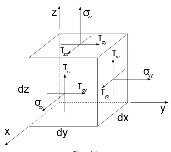
dx

dy

dz

τ

σ

x

y

z

xx

σ

xz zx

zz

zy

yz

yx xy

[image:1.595.146.486.281.583.2]

yy

Figure A.1:

A.1 Generalised Hooke’s Law for Linear Elastic Solids

If a linear elastic solid is subjected to a strain,ǫkl, the material will develop an internal

stress, denoted asσij. The stress tensor,σij, is a second rank symmetric tensor and is

defined in 3D cartesian coordinates by the relation

dFi = 3

X

j=1

(2)

where dFi are the components of a resultant force vector acting over a differential

area, which is represented by the vectordAj. The stress tensor can be represented as

a matrix, where we have replaced the cartesian x, y, z basis with indices 1, 2, 3, as

  

σ11 τ12 τ13 τ21 σ22 τ23 τ31 τ32 σ33

 

. (A.2)

The first index specifies the direction in which the stress component acts, and the second index specifies the orientation of the surface upon which it acts (Figure A.1). For an infinitesimal volume element there can no torque, which implies τ12 = τ21,

τ13=τ31, andτ23=τ32.

The strain tensor, ǫkl, is also a symmetric second rank tensor. The tensor can be

constructed from the symmetric part of the Jacobian matrix of the displacement field,

u:

ǫkl=

1 2(

∂uk ∂xl

+ ∂ul

∂xk

). (A.3)

The stress and strain are related by a 4th rank tensor, Cijkl, which is written as the

generalised form of Hooke’s Law,

σij =Cijklǫkl, (A.4)

or alternatively as

ǫij =Sijklǫkl, (A.5)

where Cijkl is known as the stiffness or elasticity tensor, and Sijkl is known as the

compliance tensor.

Since bothǫij andσklhave 9 components, we can expect thatCijklto have 81

com-ponents. However, due to symmetries in the stress and strain tensors, and the thermo-dynamic consideration of reversible stress-strain, the number of independent compo-nents in the stiffness tensor can be reduced from 81 to 21[40]. The generalised stress-strain relationship can be written in matrix form, where the components of stress and strain are written as column vectors.

           σ1 σ2 σ3 σ4 σ5 σ6            =           

(3)

§A.1 Generalised Hooke’s Law for Linear Elastic Solids 167

The stiffness in any direction can be obtained by expressing the stiffness tensor in rotated coordinates

Cpqrs=RipRjqRkrRlsCijkl, (A.7)

where R is a rotation matrix.

For isotropic linear elastic solids the stiffness matrix can be reduced to just 2 inde-pendent components [57],λandµ;

σij = 2µǫij +λtr(ǫij)δij, (A.8)

whereλ,µare the Lam´e parameters and tr(ǫij)is the trace of the strain tensor, andδij

is the Kronecker delta. We can also write the stress tensor as a linear combination of a constant tensor and symmetric traceless tensor. We can weight these respective tensor by introducing the bulk modulus, K, and the shear modulus, G:

σij = 3K(

1

3ǫkkδij) + 2G(ǫij− 1

3ǫkkδij). (A.9)

The bulk modulus of a substance, K, is thus defined as the hydrostatic pressure in-crease required to impart a relative dein-crease in the volume of the substance. The shear modulus, G, is defined as the ratio of the shear stress to shear strain.

K=−V∂P

∂V , (A.10)

G= F/A

∆x/h. (A.11)

The definitions of bulk and shear moduli are illustrated in Figure A.2.

Other related elastic moduli include Young’s modulus, E, which is the ratio of extensional stress to extensional strain. Young’s modulus is related to the bulk and shear moduli with the following equations:

K= E

3(1−2ν), (A.12)

G= E

2(1 +ν), (A.13)

whereν is the Poisson’s ratio, or the relative transverse strain divided by the relative axial strain

νyx=− ǫx ǫy

. (A.14)

(4)

[image:4.595.76.478.100.302.2]

[a] [b]

Figure A.2:[a] Bulk modulus is a constant that relates the pressure required to impart a rela-tive change in a materials volume. [b] Shear modulus is the constant relating the shear stress (or surface force) to its shear strain.

isotropic materials Poisson’s ratio is the same in all directions. That is,νxy =νyx=νxy.

A.2 Finite Element Formulation

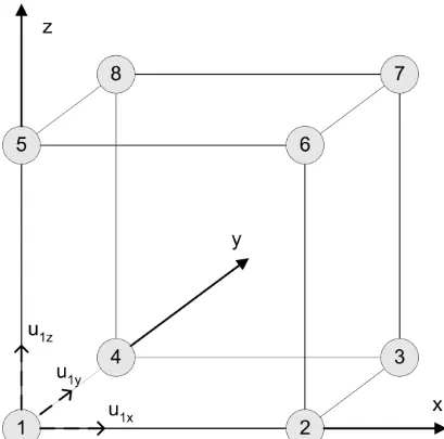
Consider an 8-noded cubic hexahedral element as shown in Figure A.3. Cubic ele-ments have the advantage of being easily applied to the coordinate system of tomo-graphic voxelated images. A displacement vectorU(x, y, z) at any point within the element can be found by interpolating the 8 nodal displacements, denoted asuij. The

displacement vector field inside the element has components U1(x, y, z),U2(x, y, z), U3(x, y, z).

U1(x, y, z) =N_ru1_r, (A.15)

U2(x, y, z) =Nru2r, (A.16)

U3(x, y, z) =Nru3r, (A.17)

where Nr is a 3×8 matrix linking the nodal displacements with the local

displace-ments within the voxel. This can be written in tensor notation:

Ui(x, y, z) =Nijkujk, (A.18)

whereNijk is a matrix of shape functions andujk is the k’th component of

(5)

[image:5.595.269.367.112.242.2]

§A.2 Finite Element Formulation 169 r Nr 1 (1-x)(1-y)(1-z) 2 x(1-y)(1-z) 3 xy(1-z) 4 (1-x)y(1-z) 5 (1-x)(1-y)z 6 x(1-y)z 7 xyz 8 (1-x)yz

Table A.1: Shape functions for individual element

shape functions are quadratic in x,y,z and are given below in Table A.1.

To calculate the strain at a point within the voxel in terms of nodal displacements were operate with a matrix of derivatives. This matrix, L, a 6×3 matrix, links the displacement to the strain;

L=            ∂

∂x 0 0

0 _∂y∂ 0 0 0 _∂z∂

∂

∂z 0 ∂x∂

0 _∂z∂ _∂y∂

∂

∂y ∂x∂ 0

           . (A.19)

Using the L operator matrix and the definition of strain as the differential change in displacement,uas a function of the coordinate axis,x,

ǫ= ∂u

∂x, (A.20)

we can write

ǫα=LαiNijkujk (A.21)

ǫα=Sαjkujk (A.22)

whereSαjkis a matrix linking the nodal displacements to a strain 6-vector within each

voxel.

To evaluate the potential energy,E, stored within a differential element,dV, that is composed of an elastic solid with stiffness tensorCijkl, we can write:

E= 1 2

Z

ǫijCijklǫkldV. (A.23)

(6)

[image:6.595.70.479.200.605.2]

(7)

§A.2 Finite Element Formulation 171

Equation A.23:

E = 1 2

Z

[Sαjkujk]TCαβ[Sβsqusq]dV, (A.24)

by grouping theS andCmatrices together

E = 1 2u

T

rpDrpsqusq, (A.25)

where

Drpsq =

Z

[Sαjk]TCαβ[Sβsq. (A.26)

The stiffness matrix,D, is evaluated for each pixel by applying Simpson’s rule. The set of nodal displacements that minimise the strain energy is found by taking the partial derivative of the strain energy equation with respect to each nodal displacement. A conjugate gradient method is used to find the set of displacements which satisfy the following equation:

∂E

(8)

(9)

Appendix B

Appendix B: Elasticity Tensors

B.1 Hip10R

Input C matrix:

0.8824 0.2402 0.2794 0.01286 -0.04285 0.02213 0.254 0.8018 0.3282 -0.005792 -0.1503 0.01408 0.2868 0.3219 1.08 -0.001149 -0.1802 0.001391 0.01017 -0.004411 0.001862 0.2688 0.007612 -0.058 -0.03181 -0.1336 -0.1756 0.006861 0.323 -0.003389 0.0253 0.01835 0.004187 -0.05865 -0.003467 0.2136

B.1.1 Orthotropic Approximation

Rotated C matrix:

0.8006 0.1473 0.4162 -0.03756 -0.001735 0.01097 0.1473 0.7917 0.2326 -0.05345 0.008713 0.02016 0.4162 0.2326 1.261 0.02614 0.002317 0.01114 -0.03756 -0.05345 0.02614 0.2784 0.009547 -0.004221 -0.001735 0.008713 0.002317 0.009547 0.3056 -0.008297 0.01097 0.02016 0.01114 -0.004221 -0.008297 0.1765 Orthotropic approximation:

0.8006 0.1473 0.4162 0 0 0 0.1473 0.7917 0.2326 0 0 0 0.4162 0.2326 1.261 0 0 0

0 0 0 0.2784 0 0

0 0 0 0 0.3056 0

0 0 0 0 0 0.1765

Deviation from Orthotropic = 7.572 percent

B.1.2 Transverse Isotropic Approximation

Rotated C matrix:

(10)

TI approximation:

0.7184 0.2184 0.3288 0 0 0 0.2184 0.7184 0.3288 0 0 0 0.3288 0.3288 1.256 0 0 0

0 0 0 0.2954 0 0

0 0 0 0 0.2954 0

0 0 0 0 0 0.25

(11)

§B.2 11R 175

B.2 11R

Input C matrix:

0.4495 0.1329 0.1555 -0.008464 -0.0141 0.01077 0.1359 0.4518 0.1828 -0.002898 -0.06472 0.008059 0.1586 0.1767 0.765 -0.02482 -0.09741 0.008499 -0.01294 -0.002887 -0.02014 0.1532 0.01083 -0.02322 -0.009585 -0.05099 -0.08988 0.01018 0.1831 -0.008721 0.01501 0.01311 0.008501 -0.02318 -0.00865 0.1051

Rotated C matrix:

0.4512 0.1068 0.1993 0.02875 -0.0004718 -0.005337 0.1068 0.4418 0.1318 0.002107 -0.006987 -0.009064 0.1993 0.1318 0.8278 -0.0086 -0.0002021 -0.006409 0.02875 0.002107 -0.0086 0.1587 -0.01368 0.0002324 -0.0004718 -0.006987 -0.0002021 -0.01368 0.1598 0.004928 -0.005337 -0.009064 -0.006409 0.0002324 0.004928 0.09562 Orthotropic approximation:

0.4512 0.1068 0.1993 0 0 0 0.1068 0.4418 0.1318 0 0 0 0.1993 0.1318 0.8278 0 0 0

0 0 0 0.1587 0 0

0 0 0 0 0.1598 0

0 0 0 0 0 0.09562

Distance from Orthotropic = 6.443 percent

Rotated C matrix:

0.4279 0.1267 0.1921 0.02658 0.007688 -0.03937 0.1267 0.431 0.1382 0.006987 -0.008648 0.02488 0.1921 0.1382 0.8276 -0.002793 -0.007124 -0.02478 0.02658 0.006987 -0.002793 0.1641 -0.01155 -0.0103 0.007688 -0.008648 -0.007124 -0.01155 0.1542 0.001471 -0.03937 0.02488 -0.02478 -0.0103 0.001471 0.1129 TI approximation:

0.4102 0.146 0.1651 0 0 0 0.146 0.4102 0.1651 0 0 0 0.1651 0.1651 0.8276 0 0 0

0 0 0 0.1592 0 0

0 0 0 0 0.1592 0

0 0 0 0 0 0.1321

(12)

B.3 15R

Input C matrix:

0.9627 0.2737 0.3082 0.009797 -0.01364 0.008302 0.2927 1.021 0.3583 -0.01444 -0.07988 -0.005164 0.2867 0.316 1.265 -0.009204 -0.108 -0.002382 0.002626 -0.002682 -0.005403 0.3072 -0.0009517 -0.02439 -0.01029 -0.05257 -0.07873 -0.0003431 0.3067 -0.01303 0.0181 0.01036 0.003652 -0.024 -0.0137 0.2131

Rotated C matrix:

1.02 0.2552 0.3356 -0.04015 -0.007206 0.006666 0.2552 0.9467 0.2676 -0.02909 -0.0004952 0.01186 0.3356 0.2676 1.308 0.002877 0.005067 0.008662 -0.04015 -0.02909 0.002877 0.2941 0.002358 -0.01208 -0.007206 -0.0004952 0.005067 0.002358 0.3136 -0.003175 0.006666 0.01186 0.008662 -0.01208 -0.003175 0.2064 Orthotropic approximation:

1.02 0.2552 0.3356 0 0 0 0.2552 0.9467 0.2676 0 0 0 0.3356 0.2676 1.308 0 0 0

0 0 0 0.2941 0 0

0 0 0 0 0.3136 0

0 0 0 0 0 0.2064

Rotated C matrix:

0.9787 0.2977 0.3293 0.04703 -0.0193 0.06793 0.2977 0.9021 0.2718 0.01628 -0.0004479 -0.06861 0.3293 0.2718 1.303 0.006819 -0.02349 0.01591 0.04703 0.01628 0.006819 0.2936 0.007028 -0.004966 -0.0193 -0.0004479 -0.02349 0.007028 0.3104 0.002313 0.06793 -0.06861 0.01591 -0.004966 0.002313 0.2558 TI approximation:

0.9076 0.3305 0.3006 0 0 0 0.3305 0.9076 0.3006 0 0 0 0.3006 0.3006 1.303 0 0 0

0 0 0 0.302 0 0

0 0 0 0 0.302 0

0 0 0 0 0 0.2886

(13)

§B.4 169R 177

B.4 169R

Input C matrix:

1.068 0.2983 0.3633 0.006548 -0.02199 0.05719 0.3734 1.113 0.468 -0.01151 -0.1207 0.04163 0.4406 0.4494 1.774 0.001031 -0.1485 0.01097 -0.004813 -0.004812 -0.01936 0.3645 0.02128 -0.0339 -0.01199 -0.082 -0.1186 0.02092 0.402 -0.01409 0.04516 0.03792 0.009899 -0.03751 -0.0139 0.2572

Rotated C matrix:

1.112 0.2742 0.478 -0.04554 -0.00651 0.02489 0.2742 1.059 0.404 0.01106 0.0004245 0.04362 0.478 0.404 1.83 0.01459 0.005668 0.01049 -0.04554 0.01106 0.01459 0.3771 0.02507 -0.006058 -0.00651 0.0004245 0.005668 0.02507 0.3764 -0.01342 0.02489 0.04362 0.01049 -0.006058 -0.01342 0.2467 Orthotropic approximation:

1.112 0.2742 0.478 0 0 0 0.2742 1.059 0.404 0 0 0 0.478 0.404 1.83 0 0 0

0 0 0 0.3771 0 0

0 0 0 0 0.3764 0

0 0 0 0 0 0.2467

Rotated C matrix:

1.122 0.2809 0.4749 0.05274 -0.01897 -0.01114 0.2809 1.046 0.4044 -0.01404 -0.002689 -0.05595 0.4749 0.4044 1.828 -0.003504 -0.03622 0.002019 0.05274 -0.01404 -0.003504 0.3735 -0.0196 -0.009373 -0.01897 -0.002689 -0.03622 -0.0196 0.3768 0.01574 -0.01114 -0.05595 0.002019 -0.009373 0.01574 0.2531 TI approximation:

1.01 0.3551 0.4397 0 0 0 0.3551 1.01 0.4397 0 0 0 0.4397 0.4397 1.828 0 0 0

0 0 0 0.3751 0 0

0 0 0 0 0.3751 0

0 0 0 0 0 0.3273

(14)

B.5 177R

Input C matrix:

0.7036 0.201 0.2266 -0.006218 -0.02282 0.008248 0.2004 0.7293 0.2565 -0.008609 -0.104 -0.005156 0.2214 0.2524 0.9423 -0.02608 -0.1136 0.004009 -0.00583 -0.005474 -0.02176 0.2154 0.004889 -0.03127 -0.0144 -0.09114 -0.1052 0.004921 0.2621 -0.009929 0.008493 -0.001813 0.005833 -0.03234 -0.009883 0.1893

Rotated C matrix:

0.7289 0.1417 0.308 0.04107 -0.001346 -0.008224 0.1417 0.6727 0.1915 0.0197 -0.001609 -0.005529 0.308 0.1915 1.029 -0.02342 0.000871 0.009612 0.04107 0.0197 -0.02342 0.2384 0.009273 0.001073 -0.001346 -0.001609 0.000871 0.009273 0.2317 0.0106 -0.008224 -0.005529 0.009612 0.001073 0.0106 0.1689 Orthotropic approximation:

0.7289 0.1417 0.308 0 0 0 0.1417 0.6727 0.1915 0 0 0 0.308 0.1915 1.029 0 0 0

0 0 0 0.2384 0 0

0 0 0 0 0.2317 0

0 0 0 0 0 0.1689

Rotated C matrix:

0.6477 0.1994 0.2476 0 0 0 0.1994 0.6477 0.2476 0 0 0 0.2476 0.2476 1.031 0 0 0

0 0 0 0.2336 0 0

0 0 0 0 0.2336 0

0 0 0 0 0 0.2241

(15)

§B.6 17R 179

B.6 17R

Input C matrix:

1.086 0.3224 0.3649 0.002533 -0.02698 -0.01932 0.327 1.033 0.3934 0.001088 -0.1016 -0.02227 0.3656 0.3864 1.484 -0.0075 -0.1294 -0.002912 -0.006747 0.005666 -0.005687 0.3001 -0.004083 -0.0314 -0.01424 -0.08388 -0.1231 -0.002716 0.3661 0.001779 -0.008447 -0.008201 -0.00481 -0.03489 0.001796 0.2623

Rotated C matrix:

1.032 0.2815 0.4271 0.05249 0.007399 0.007887 0.2815 1.058 0.3402 0.023 -0.006247 0.007927 0.4271 0.3402 1.552 -0.01794 -0.0001416 0.007197 0.05249 0.023 -0.01794 0.3459 0.003262 0.002066 0.007399 -0.006247 -0.0001416 0.003262 0.3151 0.01906 0.007887 0.007927 0.007197 0.002066 0.01906 0.2472 Orthotropic approximation:

1.032 0.2815 0.4271 0 0 0 0.2815 1.058 0.3402 0 0 0 0.4271 0.3402 1.552 0 0 0

0 0 0 0.3459 0 0

0 0 0 0 0.3151 0

0 0 0 0 0 0.2472

Rotated C matrix:

1.032 0.2834 0.4251 0.05519 0.00677 0.008498 0.2834 1.06 0.339 0.02249 -0.006562 0.006622 0.4251 0.339 1.553 -0.008107 -0.003089 0.007758 0.05519 0.02249 -0.008107 0.3445 0.003722 0.001795 0.00677 -0.006562 -0.003089 0.003722 0.3145 0.0203 0.008498 0.006622 0.007758 0.001795 0.0203 0.2479 TI approximation:

0.9795 0.3502 0.3821 0 0 0 0.3502 0.9795 0.3821 0 0 0 0.3821 0.3821 1.553 0 0 0

0 0 0 0.3295 0 0

0 0 0 0 0.3295 0

0 0 0 0 0 0.3147

(16)

B.7 180R 2K

Input C matrix:

1.433 0.4783 0.5117 -0.002933 -0.01629 -0.01454 0.51 1.5 0.5703 0.0003395 -0.1177 -0.01913 0.5471 0.5737 1.755 -0.01905 -0.1319 0.003712 0.00391 -0.0009571 -0.009427 0.4571 0.002731 -0.04298 -0.02331 -0.1229 -0.136 0.002652 0.5031 -0.00614 -0.0144 -0.01961 0.001362 -0.04311 -0.005997 0.4056

Rotated C matrix:

1.502 0.4038 0.6478 -0.04876 0.009745 -0.01247 0.4038 1.411 0.5038 -0.00768 0.0106 -0.01788 0.6478 0.5038 1.858 0.03014 -0.007202 0.003493 -0.04876 -0.00768 0.03014 0.4615 -0.001909 0.0002716 0.009745 0.0106 -0.007202 -0.001909 0.48 -0.01035 -0.01247 -0.01788 0.003493 0.0002716 -0.01035 0.3825 Orthotropic approximation:

1.502 0.4038 0.6478 0 0 0 0.4038 1.411 0.5038 0 0 0 0.6478 0.5038 1.858 0 0 0

0 0 0 0.4615 0 0

0 0 0 0 0.48 0

0 0 0 0 0 0.3825

Rotated C matrix:

1.504 0.41 0.6428 0.05544 0.01583 -0.004208 0.41 1.407 0.5028 0.007156 0.01025 0.02984 0.6428 0.5028 1.861 -0.01506 -0.003214 -0.01421 0.05544 0.007156 -0.01506 0.4597 -0.001258 -0.002492 0.01583 0.01025 -0.003214 -0.001258 0.4785 0.01249 -0.004208 0.02984 -0.01421 -0.002492 0.01249 0.3856 TI approximation:

1.387 0.4786 0.5728 0 0 0 0.4786 1.387 0.5728 0 0 0 0.5728 0.5728 1.861 0 0 0

0 0 0 0.4691 0 0

0 0 0 0 0.4691 0

0 0 0 0 0 0.4542

Deviation from TI = 8.421 percent

(17)

§B.8 180R 2K 222 181

B.8 180R 2K 222

Input C matrix:

0.9955 0.3275 0.3602 0.00289 -0.02607 -0.01348 0.3295 1.054 0.4066 -0.00308 -0.1255 -0.02141 0.3629 0.4071 1.388 -0.005914 -0.1405 0.0008195 0.003487 -0.005109 -0.007428 0.3613 0.0001235 -0.03898 -0.01979 -0.1223 -0.145 -6.144e-05 0.4137 -0.005453 -0.005815 -0.0204 0.00209 -0.03891 -0.005489 0.2997

Rotated C matrix:

1.057 0.2494 0.4849 -0.05089 0.00742 -0.01502 0.2494 0.995 0.3032 0.01438 0.005254 -0.01177 0.4849 0.3032 1.505 0.02475 -0.004775 0.007238 -0.05089 0.01438 0.02475 0.355 -0.00172 -0.003038 0.00742 0.005254 -0.004775 -0.00172 0.3799 -0.002395 -0.01502 -0.01177 0.007238 -0.003038 -0.002395 0.2806 Orthotropic approximation:

1.057 0.2494 0.4849 0 0 0 0.2494 0.995 0.3032 0 0 0 0.4849 0.3032 1.505 0 0 0

0 0 0 0.355 0 0

0 0 0 0 0.3799 0

0 0 0 0 0 0.2806

Rotated C matrix:

1.057 0.2528 0.4814 0.05769 0.00866 0.01268 0.2528 0.993 0.3029 -0.01393 0.004949 0.0138 0.4814 0.3029 1.507 -0.009817 -0.003507 -0.009431 0.05769 -0.01393 -0.009817 0.3545 0.0008431 -0.004073 0.00866 0.004949 -0.003507 0.0008431 0.3796 0.005195 0.01268 0.0138 -0.009431 -0.004073 0.005195 0.2809 TI approximation:

0.9725 0.3055 0.3921 0 0 0 0.3055 0.9725 0.3921 0 0 0 0.3921 0.3921 1.507 0 0 0

0 0 0 0.3671 0 0

0 0 0 0 0.3671 0

0 0 0 0 0 0.3335

(18)

B.9 180R 2K 444

Input C matrix:

0.5062 0.1334 0.1774 0.01135 -0.008148 0.001146 0.1272 0.5547 0.2189 -0.001341 -0.09413 -0.00296 0.1916 0.238 0.9785 -0.0008432 -0.1308 0.005834 0.01958 -0.003241 0.0006309 0.2481 0.007618 -0.02172 0.0008535 -0.07066 -0.1135 0.009456 0.2917 -0.00519 0.004677 0.005463 0.01057 -0.02158 -0.005167 0.1839

Rotated C matrix:

0.5544 0.1024 0.2698 -0.02606 -0.00196 0.001071 0.1024 0.5374 0.1207 0.04749 0.02235 0.01261 0.2698 0.1207 1.068 0.003912 -0.001357 0.007785 -0.02606 0.04749 0.003912 0.2307 0.001115 0.001084 -0.00196 0.02235 -0.001357 0.001115 0.2548 0.002109 0.001071 0.01261 0.007785 0.001084 0.002109 0.1778 Orthotropic approximation:

0.5544 0.1024 0.2698 0 0 0 0.1024 0.5374 0.1207 0 0 0 0.2698 0.1207 1.068 0 0 0

0 0 0 0.2307 0 0

0 0 0 0 0.2548 0

0 0 0 0 0 0.1778

Distance from Orthotropic = 7.617 percent

Rotated C matrix:

0.5547 0.1043 0.2671 0.03364 -0.006024 -0.003159 0.1043 0.5305 0.1281 -0.0455 0.02124 -0.0094 0.2671 0.1281 1.065 0.01686 -0.006728 -0.009965 0.03364 -0.0455 0.01686 0.2359 -0.002004 -0.001234 -0.006024 0.02124 -0.006728 -0.002004 0.2548 0.001788 -0.003159 -0.0094 -0.009965 -0.001234 0.001788 0.1775 TI approximation:

0.5218 0.1251 0.1976 0 0 0 0.1251 0.5218 0.1976 0 0 0 0.1976 0.1976 1.065 0 0 0

0 0 0 0.2453 0 0

0 0 0 0 0.2453 0

0 0 0 0 0 0.1983

(19)

§B.10 180R 2K 888 183

B.10 180R 2K 888

Input C matrix:

0.3387 0.06879 0.1095 0.01504 -0.0006781 0.001039 0.06327 0.3589 0.148 -0.00701 -0.05848 0.00475 0.08743 0.1208 0.5621 0.002797 -0.0623 0.00867 0.01589 -0.007548 0.001783 0.1886 0.00657 -0.01707 0.006104 -0.04194 -0.05076 0.006583 0.2162 -0.001532 0.003062 0.004994 0.009058 -0.01707 -0.003097 0.142

Rotated C matrix:

0.3582 0.04848 0.1438 0.009387 -0.0003845 0.0009753 0.04848 0.3853 0.03107 -0.03735 -0.01655 0.01249 0.1438 0.03107 0.6175 -0.004882 0.00197 0.006568 0.009387 -0.03735 -0.004882 0.1648 -0.0008508 -0.002159 -0.0003845 -0.01655 0.00197 -0.0008508 0.1938 -0.006214 0.0009753 0.01249 0.006568 -0.002159 -0.006214 0.1375 Orthotropic approximation:

0.3582 0.04848 0.1438 0 0 0 0.04848 0.3853 0.03107 0 0 0 0.1438 0.03107 0.6175 0 0 0

0 0 0 0.1648 0 0

0 0 0 0 0.1938 0

0 0 0 0 0 0.1375

Rotated C matrix:

0.3595 0.05303 0.1368 0.02607 -0.01074 -0.002451 0.05303 0.3565 0.05352 -0.03414 0.01841 -0.006999 0.1368 0.05352 0.6051 0.03098 -0.00391 -0.007216 0.02607 -0.03414 0.03098 0.1852 -0.002833 0.001074 -0.01074 0.01841 -0.00391 -0.002833 0.1938 0.004468 -0.002451 -0.006999 -0.007216 0.001074 0.004468 0.1371 TI approximation:

0.3503 0.06073 0.09518 0 0 0 0.06073 0.3503 0.09518 0 0 0 0.09518 0.09518 0.6051 0 0 0

0 0 0 0.1895 0 0

0 0 0 0 0.1895 0

0 0 0 0 0 0.1448

(20)

B.11 180R 1K

Input C matrix:

0.795 0.2293 0.2507 -0.002195 -0.02393 -0.008778 0.2368 0.8276 0.288 -0.004045 -0.1049 -0.02024 0.2546 0.2835 1.065 -0.005396 -0.1222 -0.0005557 -0.003249 -0.00261 -0.006657 0.2437 -0.000505 -0.03266 -0.01442 -0.09039 -0.124 -0.000712 0.3067 -0.003193 -0.003076 -0.01093 0.003795 -0.03293 -0.002385 0.2051

Rotated C matrix:

0.8287 0.1718 0.3409 -0.04136 0.003487 -0.008722 0.1718 0.768 0.2167 -0.01374 -0.001283 -0.008263 0.3409 0.2167 1.161 0.02033 -0.001152 0.004315 -0.04136 -0.01374 0.02033 0.272 -0.0001663 0.00157 0.003487 -0.001283 -0.001152 -0.0001663 0.2613 -0.007962 -0.008722 -0.008263 0.004315 0.00157 -0.007962 0.1871 Orthotropic approximation:

0.8287 0.1718 0.3409 0 0 0 0.1718 0.768 0.2167 0 0 0 0.3409 0.2167 1.161 0 0 0

0 0 0 0.272 0 0

0 0 0 0 0.2613 0

0 0 0 0 0 0.1871

Rotated C matrix:

0.8283 0.1741 0.3387 0.04597 0.002644 0.008055 0.1741 0.7701 0.215 0.01358 -0.002226 0.007808 0.3387 0.215 1.163 -0.009554 -0.00579 -0.003767 0.04597 0.01358 -0.009554 0.2702 0.001417 -8.189e-05 0.002644 -0.002226 -0.00579 0.001417 0.261 0.01014 0.008055 0.007808 -0.003767 -8.189e-05 0.01014 0.1875 TI approximation:

0.7367 0.2366 0.2769 0 0 0 0.2366 0.7367 0.2769 0 0 0 0.2769 0.2769 1.163 0 0 0

0 0 0 0.2656 0 0

0 0 0 0 0.2656 0

0 0 0 0 0 0.2501

(21)

§B.12 19R 185

B.12 19R

Input C matrix:

0.4735 0.1325 0.156 0.01282 -0.0183 0.002054 0.1383 0.4906 0.1927 0.002911 -0.07842 -0.00457 0.1554 0.1851 0.7736 0.009426 -0.09968 0.0001561 0.01034 0.003393 0.009299 0.1627 -0.0004501 -0.02513 -0.005985 -0.06563 -0.09272 -0.0004355 0.1946 0.004522 -0.0006476 -0.004145 5.939e-05 -0.02521 0.004314 0.1245

Rotated C matrix:

0.4902 0.09658 0.2198 -0.03517 0.002075 0.002188 0.09658 0.4649 0.1244 -6.991e-05 0.007226 0.002841 0.2198 0.1244 0.8351 0.0147 -0.001038 0.0009265 -0.03517 -6.991e-05 0.0147 0.1687 -0.004442 8.328e-05 0.002075 0.007226 -0.001038 -0.004442 0.1742 -0.008123 0.002188 0.002841 0.0009265 8.328e-05 -0.008123 0.1127 Orthotropic approximation:

0.4902 0.09658 0.2198 0 0 0 0.09658 0.4649 0.1244 0 0 0 0.2198 0.1244 0.8351 0 0 0

0 0 0 0.1687 0 0

0 0 0 0 0.1742 0

0 0 0 0 0 0.1127

Rotated C matrix:

0.4836 0.1071 0.2159 0.03709 -0.006711 0.02202 0.1071 0.456 0.126 0.00232 0.01012 -0.02299 0.2159 0.126 0.8359 -0.005026 -0.0008391 0.01404 0.03709 0.00232 -0.005026 0.1695 0.004943 0.007281 -0.006711 0.01012 -0.0008391 0.004943 0.1722 0.007101 0.02202 -0.02299 0.01404 0.007281 0.007101 0.1212 TI approximation:

0.4397 0.1371 0.171 0 0 0 0.1371 0.4397 0.171 0 0 0 0.171 0.171 0.8359 0 0 0

0 0 0 0.1709 0 0

0 0 0 0 0.1709 0

0 0 0 0 0 0.1513

(22)

B.13 45R

Input C matrix:

1.164 0.3697 0.3965 -0.03202 -0.02027 -0.02704 0.3706 1.234 0.4354 -0.007053 -0.09989 -0.02099 0.3353 0.371 1.527 -0.0474 -0.1395 -0.005261 -0.009897 0.0087 -0.007838 0.3131 -0.0002889 -0.03105 -0.01163 -0.1008 -0.1407 0.0003878 0.3212 -0.004037 -0.01589 -0.01388 -0.00073 -0.03391 -0.01039 0.2692

Rotated C matrix:

1.233 0.3226 0.4151 -0.08922 0.008054 -0.01592 0.3226 1.129 0.3221 -0.06285 -0.005249 -0.02115 0.4151 0.3221 1.595 -0.003182 -2.136e-05 0.00139 -0.08922 -0.06285 -0.003182 0.306 0.003316 -0.004477 0.008054 -0.005249 -2.136e-05 0.003316 0.3246 -0.02021 -0.01592 -0.02115 0.00139 -0.004477 -0.02021 0.2566 Orthotropic approximation:

1.233 0.3226 0.4151 0 0 0 0.3226 1.129 0.3221 0 0 0 0.4151 0.3221 1.595 0 0 0

0 0 0 0.306 0 0

0 0 0 0 0.3246 0

0 0 0 0 0 0.2566

Rotated C matrix:

1.235 0.333 0.4119 0.09087 0.01676 -0.00916 0.333 1.126 0.317 0.05763 -0.00468 0.03814 0.4119 0.317 1.594 0.02055 -0.001153 -0.007007 0.09087 0.05763 0.02055 0.3031 -0.00382 -0.008291 0.01676 -0.00468 -0.001153 -0.00382 0.3236 0.0202 -0.00916 0.03814 -0.007007 -0.008291 0.0202 0.2613 TI approximation:

1.099 0.4143 0.3644 0 0 0 0.4143 1.099 0.3644 0 0 0 0.3644 0.3644 1.594 0 0 0

0 0 0 0.3133 0 0

0 0 0 0 0.3133 0

0 0 0 0 0 0.3426

(23)

§B.14 72R 187

B.14 72R

Input C matrix:

0.4519 0.1273 0.1478 0.02032 -0.00984 0.01237 0.1301 0.4158 0.172 0.004807 -0.04935 0.01639 0.142 0.1618 0.6828 0.02374 -0.072 0.002288 0.01121 0.005004 0.02528 0.09475 -0.003 -0.01104 -0.002744 -0.031 -0.05617 0.003623 0.151 0.003941 0.008483 0.008139 -0.001517 -0.01697 0.004096 0.1008

Rotated C matrix:

0.4447 0.1103 0.1273 -0.007052 0.008575 0.01201 0.1103 0.4145 0.1726 -0.006465 0.02042 0.01341 0.1273 0.1726 0.7164 -0.001597 -0.003431 0.0002339 -0.007052 -0.006465 -0.001597 0.09973 0.0004376 0.01643 0.008575 0.02042 -0.003431 0.0004376 0.1396 0.00183 0.01201 0.01341 0.0002339 0.01643 0.00183 0.09464 Orthotropic approximation:

0.4447 0.1103 0.1273 0 0 0 0.1103 0.4145 0.1726 0 0 0 0.1273 0.1726 0.7164 0 0 0

0 0 0 0.09973 0 0

0 0 0 0 0.1396 0

0 0 0 0 0 0.09464

Rotated C matrix:

0.4159 0.1375 0.171 0.01958 -0.005527 0.01501 0.1375 0.4048 0.1282 0.01258 0.009749 -0.04475 0.171 0.1282 0.7161 0.001259 0.004875 0.01241 0.01958 0.01258 0.001259 0.1364 -0.008968 0.008081 -0.005527 0.009749 0.004875 -0.008968 0.1025 0.007767 0.01501 -0.04475 0.01241 0.008081 0.007767 0.1145 TI approximation:

0.3994 0.1485 0.1496 0 0 0 0.1485 0.3994 0.1496 0 0 0 0.1496 0.1496 0.7161 0 0 0

0 0 0 0.1194 0 0

0 0 0 0 0.1194 0

0 0 0 0 0 0.1254

(24)

B.15 9R

Input C matrix:

0.5317 0.1478 0.1787 -0.009798 -0.01679 0.01048 0.1535 0.5031 0.194 -0.006151 -0.05949 0.004017 0.1772 0.1857 0.7669 -0.01821 -0.083 0.002232 -0.008323 -0.002527 -0.01374 0.1685 0.004785 -0.02018 -0.01322 -0.04908 -0.07403 0.004939 0.1814 -0.005809 0.00798 0.004341 0.003012 -0.02084 -0.005716 0.1325

Rotated C matrix:

0.5022 0.1226 0.2084 0.02947 0.0006607 0.0003617 0.1226 0.512 0.1622 0.01817 -0.004214 -0.001464 0.2084 0.1622 0.8146 -0.009763 0.0009604 -0.003396 0.02947 0.01817 -0.009763 0.1695 -0.007706 -0.001612 0.0006607 -0.004214 0.0009604 -0.007706 0.1759 0.00685 0.0003617 -0.001464 -0.003396 -0.001612 0.00685 0.1236 Orthotropic approximation:

0.5022 0.1226 0.2084 0 0 0 0.1226 0.512 0.1622 0 0 0 0.2084 0.1622 0.8146 0 0 0

0 0 0 0.1695 0 0

0 0 0 0 0.1759 0

0 0 0 0 0 0.1236

Rotated C matrix:

0.4733 0.1574 0.1849 0 0 0 0.1574 0.4733 0.1849 0 0 0 0.1849 0.1849 0.8145 0 0 0

0 0 0 0.1724 0 0

0 0 0 0 0.1724 0

0 0 0 0 0 0.1579

(25)

§B.16 A08R 189

B.16 A08R

Input C matrix:

0.4378 0.1374 0.1553 0.01434 -0.01203 0.006874 0.1405 0.4905 0.1876 0.001922 -0.07913 0.001362 0.1535 0.182 0.6686 0.01687 -0.09635 0.0001238 0.007175 0.001057 0.01361 0.1447 0.0005581 -0.02289 -0.006377 -0.06491 -0.08866 0.0003136 0.1805 0.002407 0.006367 0.003531 -0.002066 -0.02328 0.00208 0.1277

Rotated C matrix:

0.4908 0.09726 0.2196 0.03067 -0.003167 -0.006575 0.09726 0.432 0.1172 0.002339 0.003862 -0.00967 0.2196 0.1172 0.7412 -0.01455 0.0008014 -0.0001042 0.03067 0.002339 -0.01455 0.1479 0.0006981 -0.002329 -0.003167 0.003862 0.0008014 0.0006981 0.1573 0.01057 -0.006575 -0.00967 -0.0001042 -0.002329 0.01057 0.1142 Orthotropic approximation:

0.4908 0.09726 0.2196 0 0 0 0.09726 0.432 0.1172 0 0 0 0.2196 0.1172 0.7412 0 0 0

0 0 0 0.1479 0 0

0 0 0 0 0.1573 0

0 0 0 0 0 0.1142

Rotated C matrix:

0.488 0.1059 0.2168 0.03336 -0.01012 0.01441 0.1059 0.4229 0.1175 0.002955 0.007127 -0.02263 0.2168 0.1175 0.742 -0.004014 0.00323 0.01366 0.03336 0.002955 -0.004014 0.1477 0.001326 0.004908 -0.01012 0.007127 0.00323 0.001326 0.1563 0.009454 0.01441 -0.02263 0.01366 0.004908 0.009454 0.1211 TI approximation:

0.4286 0.1327 0.1672 0 0 0 0.1327 0.4286 0.1672 0 0 0 0.1672 0.1672 0.742 0 0 0

0 0 0 0.152 0 0

0 0 0 0 0.152 0

0 0 0 0 0 0.1479

(26)

B.17 A3R

Input C matrix:

0.701 0.1971 0.2388 -0.003313 -0.02831 -0.006959 0.2052 0.7071 0.2814 0.0001088 -0.1115 -0.01245 0.2398 0.2745 1.08 -0.01864 -0.1457 0.001547 -0.009354 -0.002068 -0.02254 0.24 0.001891 -0.03644 -0.01707 -0.09809 -0.142 0.001424 0.287 -0.002408 -0.004219 -0.008146 0.002308 -0.03669 -0.00264 0.1862

Rotated C matrix:

0.7091 0.1407 0.3296 0.04517 0.008924 0.009068 0.1407 0.6804 0.1927 0.006074 -0.004556 0.011 0.3296 0.1927 1.188 -0.01989 -0.0046 0.001515 0.04517 0.006074 -0.01989 0.2444 -0.001435 0.002619 0.008924 -0.004556 -0.0046 -0.001435 0.2559 0.008301 0.009068 0.011 0.001515 0.002619 0.008301 0.1686 Orthotropic approximation:

0.7091 0.1407 0.3296 0 0 0 0.1407 0.6804 0.1927 0 0 0 0.3296 0.1927 1.188 0 0 0

0 0 0 0.2444 0 0

0 0 0 0 0.2559 0

0 0 0 0 0 0.1686

Rotated C matrix:

0.6414 0.1964 0.26 0 0 0 0.1964 0.6414 0.26 0 0 0 0.26 0.26 1.189 0 0 0

0 0 0 0.2496 0 0

0 0 0 0 0.2496 0

0 0 0 0 0 0.2225

(27)

§B.18 Artibone256 191

B.18 Artibone256

Input C matrix:

0.7163 0.1087 0.107 -0.0008219 -0.00212 -0.0005858 0.1087 0.7234 0.1085 -0.0008288 -0.0006772 -0.001855 0.1069 0.1084 0.6904 -0.0002086 -0.0005007 -0.0002755 -0.0008257 -0.0008327 -0.0002079 0.2835 -0.000461 -0.0005085 -0.00213 -0.0006788 -0.0005052 -0.0004628 0.264 -0.0001352 -0.0005842 -0.001863 -0.0002805 -0.0005085 -0.0001356 0.2692

Rotated C matrix:

0.6903 0.1085 0.1069 -0.0002677 0.001247 0.0004401 0.1085 0.7235 0.1087 -0.001018 0.0006888 9.282e-05 0.1069 0.1087 0.7164 -0.00128 0.001092 0.0007961 -0.0002677 -0.001018 -0.00128 0.2692 5.537e-05 0.0007029 0.001247 0.0006888 0.001092 5.537e-05 0.264 -0.0002678 0.0004401 9.282e-05 0.0007961 0.0007029 -0.0002678 0.2835 Orthotropic approximation:

0.6903 0.1085 0.1069 0 0 0 0.1085 0.7235 0.1087 0 0 0 0.1069 0.1087 0.7164 0 0 0

0 0 0 0.2692 0 0

0 0 0 0 0.264 0

0 0 0 0 0 0.2835

Rotated C matrix:

0.7235 0.1084 0.1087 0.0006809 0.001207 -0.0008305 0.1084 0.6904 0.107 0.001063 0.0002682 -0.0002123 0.1087 0.107 0.7164 0.001322 0.00116 -0.000822 0.0006809 0.001063 0.001322 0.264 -0.0001337 0.0003029 0.001207 0.0002682 0.00116 -0.0001337 0.2692 0.0006512 -0.0008305 -0.0002123 -0.000822 0.0003029 0.0006512 0.2835 TI approximation:

0.6991 0.1163 0.1078 0 0 0 0.1163 0.6991 0.1078 0 0 0 0.1078 0.1078 0.7164 0 0 0

0 0 0 0.2666 0 0

0 0 0 0 0.2666 0

0 0 0 0 0 0.2914

(28)

(29)

Bibliography

1. ALEXANDER, R. M. Optima for Animals. Edward Arnold, London, 1982.

2. ANNAZ, B., HING, K., KAYSER, M., BUCKLAND, T., AND DI SILVIO, L.

Poros-ity variation in hydroxyapatite and osteoblast morphology: a scanning electron microscopy study. Journal of Microscopy 215, 1 (2004), 100–110.

3. ARNS, C., KNACKSTEDT, M., PINCZEWSKI, W., AND GARBOCZI, E.

Compu-tation of linear elastic properties from microtomographic images: methodology and agreement between theory and experiment. Geophysics 67, 5 (2002), 1396– 1405.

4. ARNS, C. H. The Influence of Morphology on Physical Properties of Reservoir Rocks. PhD thesis, School of Petroleum Engineering, University of New South Wales, Sydney, Australia, 2002.

5. ARNS, C. H., KNACKSTEDT, M. A., PINCZEWSKI, W. V., ANDMARTYS, N. Vir-tual permeametry on microtomographic images. Journal of Petroleum Science and Engineering 45, 1-2 (2004), 41–46.

6. ASCENZI, A., AND BONUCCI, E. The tensile properties of single osteons. The Anatomical Record 158, 4 (1967), 375–386.

7. ASHMAN, R. B., AND RHO, J. Y. Elastic modulus of trabecular bone material.

Journal of Biomechanics 21(1988), 177–181.

8. ASHMAN, R. B., RHO, J. Y., AND TURNER, C. H. Anatomical variation of

or-thotropic elastic moduli of the proximal human tibia. Journal of Biomechanics 22, 8-9 (1989), 895–900.

9. AUGAT, P., REEB, H., AND CLAES, L. Prediction of fracture load at different

skeletal sites by geometric properties of the cortical shell. Journal of Bone and Mineral Research 11, 9 (1996), 1356–1363.

10. BEAUPRE´, G. S.,ANDCARTER, D. R. Finite element analysis in biomechanics. In

(30)

11. BEAUPRE, G. S., AND HAYES, W. C. Finite element analysis of a three-dimensional open-celled model for trabecular bone. Journal of Biomechanical En-gineering 107, 3 (1985), 249–256.

12. BECK, J. D., CANFIELD, B. L., HADDOCK, S. M., CHEN, T. J. H., KOTHARI, M.,

AND KEAVENY, T. M. Three-dimensional imaging of trabecular bone using the computer numerically controlled milling technique. Bone 21, 3 (1997), 281–287.

13. BELL, E. Tissue engineering in perspective. In Lanza et al. [141], pp. xxxv–xli. 14. BELL, G. H., DUNBAR, O., BECK, J. S.,ANDGIBB, A. Variations in strength of

vertebrae with age and their relation to osteoporosis. Calcified Tissue International 1, 1 (1967), 75–86.

15. BIGNON, A., CHOUTEAU, J., CHEVALIER, J., FANTOZZI, G., CARRET, J., CHAVASSIEUX, P., BOIVIN, G., MELIN, M., AND HARTMANN, D. Effect of micro- and macroporosity of bone substitutes on their mechanical properties and cellular response. Journal of Materials Science: Materials in Medicine 14, 12 (2003), 1089–1097.

16. BLUNT, M. J. Flow in porous media – pore-network models and multiphase flow. Current Opinion in Colloid and Interface Science 6, 3 (2001), 197–207.

17. BOHNER, M., AND BAUMGART, F. Theoretical model to determine the effects of geometrical factors on the resorption of calcium phosphate bone substitutes.

Biomaterials 25, 17 (2004), 3569–3582.

18. BONFIELD, W. Designing porous scaffolds for tissue engineering. Philosophical Transactions of the Royal Society A 364, 1838 (2006), 227–232.

19. BOONEN, S., CHENG, X., NICHOLSON, P., VERBEKE, G., BROOS, P., AND DE

-QUEKER, J. The accuracy of peripheral skeletal assessment at the radius in

esti-mating femoral bone density as measured by dual-energy x-ray absorptiometry: a comparative study of single-photon absorptiometry and computed tomogra-phy.Journal of Internal Medicine 242, 4 (1997), 323–328.

20. BOSKEY, A. L. Bone mineralization. In Cowin [37], pp. 5.8–5.20.

(31)

Bibliography 195

22. BOYDE, A., JONES, S. J., AERSSENS, J., AND DEQUEKER, J. Mineral density quantitation of the human cortical iliac crest with backscattered electron image analysis: variations with age, sex, and degree of osteoarthritis. Bone 6, 6 (1995), 619–627.

23. BRADLEY, D. A., CHONG, C. S., AND GHOSE, A. M. Photon absorptiometric studies of elements, mixtures and substances of biomedical interest. Physics in Medicine and Biology 31, 3 (1986), 267–273.

24. BROOKS, R.,ANDCHIRO, G. D. Beam hardening in x-ray reconstructive

tomog-raphy. Physics in Medicine and Biology 21, 3 (1976), 390–398.

25. BROWN, T. D.,ANDFERGUSON, A. B. The development of computational stress analysis of the femoral head. The Journal of Bone and Joint Surgery [Am] 60A(1978), 619–629.

26. CAPES, J., ANDO, H., AND CAMERON, R. Fabrication of polymeric scaffolds

with controlled distribution of pores. Journal of Materials Science: Materials in Medicine 16, 12 (2005), 1069–1075.

27. CARMAN, P. C. Flow of gases through porous media. Butterworths, London, 1956. 28. CARTER, D. R.,ANDHAYES, W. C. Bone compressive strength: The influence of

density and strain rate.Science 194, 4270 (1976), 1174–1176.

29. CARTER, D. R., AND HAYES, W. C. The compressive behavior of bone as a two-phase porous structure. The Journal of Bone and Joint Surgery 59-A, 7 (1977), 954–962.

30. CHADWICK, P., VIANELLO, M.,ANDCOWIN, S. C. A new proof that the

num-ber of linear elastic symmetries is eight. Journal of the Mechanics and Physics of Solids 49, 11 (2001), 2471–2492.

31. CHENG, X. G., LOWET, G., BOONEN, S., NICHOLSON, P. H. F., BRYS, P., NUS, J., AND DEQUEKER, J. Assessment of the strength of proximal femur in vitro:

relationship to femoral bone mineral density and femoral geometry. Bone 20, 3 (1997), 213–218.

(32)

33. CIOFFI, M., BOSCHETTI, F., RAIMONDI, M. T.,ANDDUBINI, G. Modeling eval-uation of the fluid-dynamic microenvironment in tissue-engineered constructs: A micro-CT based model.Biotechnology and Bioengineering 93, 3 (2006), 500–510.

34. COOPER, C. The crippling consequences of fractures and their impact on quality

of life. American Journal of Medicine 103, 2A (1997), 12S–19S.

35. COOPER, D., TURINSKY, A., SENSEN, C., AND HALLGRIMSSON, B. Effect of

voxel size on 3D micro-CT analysis of cortical bone porosity. Calcified Tissue In-ternational 80, 3 (2007), 211–219.

36. COURTNEY, A. C., WACHTEL, E. F., MYERS, E. R.,ANDHAYES, W. C. Effects of loading rate on strength of the proximal femur. Calcified Tissue International 55, 1 (1994), 53–58.

37. COWIN, S. C., Ed.Bone Mechanics Handbook(Boca Raton, 2001), CRC Press. 38. COWIN, S. C. The false premise in Wolff’s law. In Cowin [37], pp. 30.1–30.15. 39. COWIN, S. C. Mechanics of materials. In Cowin [37], pp. 6.1–6.24.

40. COWIN, S. C.,ANDMEHRABADI, M. M. On the identification of material sym-metry for anisotropic elastic constants. Quarterly Journal Of Mechanics And Ap-plied Mathematics 40, 4 (1987), 451–476.

41. COWIN, S. C.,AND MEHRABADI, M. M. Identification of the elastic symmetry

of bone and other materials. Journal of Biomechanics 22, 6-7 (1989), 503–515.

42. CRAWFORD, R. P., CANN, C. E., AND KEAVENY, T. M. Finite element models

better predict in vitro vertebral body compressive strength better than quantita-tive computed tomography. Bone 33, 4 (2003), 744–750.

43. CUMMINGS, S. R. Epidemiologic studies of osteoporotic fractures: method-ologic studies.Calcified Tissue International 49, 1 (1991), S15–S20.

44. CURREY, J. D. Power law models for the mechanical properties of cancellous bone. Engineering in Medicine 15, 3 (1986), 153–154.

45. CURREY, J. D. Bones, Structure and Mechanics, first ed. Princeton University Press, New Jersey, 2002.

(33)

47. DEMES, B., JUNGERS, W., AND SELPIEN, K. Body size, locomotion and long bone cross sectional geometry in indriid primates. American Journal of Physical Anthropology 86, 4 (1991), 537–547.

48. DING, M., ODGAARD, A., LINDE, F.,ANDHVID, I. Age-related variations in the microstructure of human tibial cancellous bone. Journal of Orthopaedic Research 20, 3 (2002), 615–621.

49. DOERNBERG, M., VON RECHENBERG, B., BOHNER, M., GRUNENFELDER, S., VAN LENTHE, G., MULLER, R., GASSER, B., MATHYS, R., BAROUD, G., AND

AUER, J. In vivo behavior of calcium phosphate scaffolds with four different pore sizes.Biomaterials 27, 30 (2006), 5186–5198.

50. DUAN, Y., BECK, T. J., WANG, X.-F., AND SEEMAN, E. Structural and biome-chanical basis of sexual dimorphism in femoral neck fragility has its origins in growth and aging. Journal of Bone and Mineral Research 18, 10 (2003), 1766–1774.

51. DUNCAN, R. L., ANDTURNER, C. H. Mechanotransduction and the functional response of bone to mechanical strain. Calcified Tissue International 57, 5 (1995), 344–358.

52. ESWARAN, S. K., GUPTA, A., AND KEAVENY, T. M. Locations of bone tissue at high risk of initial failure during compressive loading of the human vertebral body. Bone 41, 4 (2007), 733–739.

53. FELDKAMP, L. A. Practical cone-beam algorithm. Journal of The Optical Society of America A 1, 6 (1984), 612–619.

54. FELDKAMP, L. A.,ANDDAVIS, L. C. Topology and elastic properties of depleted media. Physical Review B 37, 7 (1988), 3448–3453.

55. FELDKAMP, L. A., GOLDSTEIN, S., PARFITT, A., JESION, G.,ANDKLEEREKOPER,

M. The direct examination of three-dimensional bone architecture in vitro by computed tomography. Journal of Bone and Mineral Research 4, 1 (1989), 3–11.

56. FERGUSON, V. L., BUSHBY, A. J., AND BOYDE, A. Nanomechanical properties and mineral concentration in articular calcified cartilage and subchondral bone.

Journal of Anatomy 203(2003), 191–202.

(34)

58. FILARDI, S., ZEBAZE, R. M. D., DUAN, Y., EDMONDS, J., BECK, T., AND SEE

-MAN, E. Femoral neck fragility in women has its structural and biomechanical

basis established by periosteal modeling during growth and endocortical remod-eling during aging.Osteoporosis International 15, 2 (2004), 103–107.

59. FLANNERY, B. P., DECKMAN, H. W., ROBERGE, W. G., AND D’AMICO, K. L.

Three-dimensional x-ray microtomography. Science 237, 4821 (1987), 1439–1444.

60. GARBOCZI, E., AND DAY, A. An algorithm for computing the effective linear elastic properties of heterogeneous materials: Three-dimensional results for com-posites with equal phase Poisson ratios. Journal of the Mechanics and Physics of Solids 43, 9 (1995), 1349–1362.

61. GARBOCZI, E. J. Finite element and finite difference programs for computing

the linear electric and elastic properties of digital images of random materials. Tech. Rep. 6269, National Institute of Standards and Technology, Gaithersburg, Maryland, December 1998.

62. GAUTHIER, O., BOULER, J., AGUADO, E., PILET, P., ANDDACULSI, G. Macro-porous biphasic calcium phosphate ceramics: influence of macropore diameter and macroporosity percentage on bone ingrowth. Biomaterials 19, 1-3 (1998), 133– 139.

63. GAUTHIER, O., M ¨ULLER, R.,VONSTECHOW, D., LAMY, B., WEISS, P., BOULER,

J.-M., AGUADO, E.,ANDDACULSI, G. In vivo bone regeneration with injectable calcium phosphate biomaterial: A three dimensional micro computed tomo-graphic, biomechanical and sem study.Biomaterials 26, 27 (2005), 5444–5453.

64. GIANGREGORIO, L. M., ANDMCCARTNEY, N. Reduced loading due to spinal-cord injury at birth results in ‘slender’ bones: a case study. Osteoporosis Interna-tional 18, 1 (2007), 117–120.

65. GIBSON, L. J.,ANDASHBY, M. F. Cellular Solids: Structures and Properties. Perg-amon Press, Oxford, 1988.

66. GIBSON, L. J.,ANDASHBY, M. F. Cellular Solids: Structures and Properties, 2nd ed.

Pergamon, Oxford, 1997.

67. GILMORE, R. S., ANDKATZ, J. L. Elastic properties of apatites. Journal of Mate-rials Science 17, 4 (1982), 1131–1141.

(35)

69. GROVES, E. W. H. Experimental principles of the operative treatment of frac-tures and their clinical application. Lancet 4720(Feb 1914), 435–441.

70. GULDBERG, R. E., HOLLISTER, S. J., AND CHARRAS, G. T. The accuracy of digital image-based finite element models. Journal of Biomechanical Engineering 120, 2 (1998), 289–295.

71. HARA, T., TANCK, E., HOMMINGA, J., ANDHUISKES, R. The influence of mi-crocomputed tomography threshold variations on the assessment of structural and mechanical trabecular bone properties.Bone 31, 1 (2002), 107–109.

72. HARRIGAN, T. P., JASTY, M., MANN, R. W., ANDHARRIS, W. H. Limitations of the continuum assumption in cancellous bone. Journal of Biomechanics 21, 4 (1988), 269–275.

73. HAYES, W. C., MYERS, E. R., MORRIS, J. N., GERHART, T. N., YETT, H. S.,AND

LIPSITZ, L. A. Impact near the hip dominates fracture risk in elderly nursing home residents who fall. Calcified Tissue International 52, 3 (1993), 192–198.

74. HELBIG, K. Simultaneous observation of seismic waves of different polarization

indicates subsurface anisotropy and might help to unravel its cause. Journal of Applied Geophysics 30, 1-2 (1993), 1–24.

75. HENCH, L. Bioceramics: From concept to clinic. Journal of American Ceramic

Society 74, 7 (1991), 1487–1510.

76. HENCH, L. L., AND POLAK, J. M. Third-generation biomedical materials. Sci-ence 295, 5557 (2002), 1014–1017.

77. HENRY, Y. M.,ANDEASTELL, R. Ethnic and gender differences in bone mineral density and bone turnover in young adults: Effect of bone size. Osteoporosis International 11, 6 (2000), 512–517.

78. HERNANDEZ, C. J.,ANDKEAVENY, T. M. A biomechanical perspective on bone quality. Bone 29, 6 (2006), 1173–1181.

79. HILDEBRAND, T., AND R ¨UEGSEGGER, P. A new method for the

model-independent assessment of thickness in three-dimensional images. Journal of Microscopy 185, 1 (1997), 67–75.

80. HILPERT, M., AND MILLER, C. T. Pore-morphology based simulation of

(36)

81. HING, K., BEST, S., TANNER, K., BONFIELD, W., ANDREVELL, P. Quantifica-tion of bone ingrowth within bone derived porous hydroxyapatite implants of varying density. Journal of Materials Science: Materials in Medicine 10, 10-11 (1999), 663–670.

82. HING, K., BEST, S., TANNER, K., BONFIELD, W., AND REVELL, P. Mediation of bone ingrowth in porous hydroxyapatite bone graft substitutes. Journal of Biomedical Materials Research A 68, 1 (2004), 187–200.

83. HING, K. A. Bioceramic bone graft substitutes: Influence of porosity and chem-istry. International Journal of Applied Ceramic Technology 2, 3 (2005), 184–199.

84. HO, S.,ANDHUTMACHER, D. A comparison of micro CT with other techniques used in the characterization of scaffolds. Biomaterials 27, 8 (2006), 1362–1376.

85. HOC, T., HENRY, L., VERDIER, M., AUBRY, D., SEDEL, L., AND MEUNIER, A.

Effect of microstructure on the mechanical properties of haversian cortical bone.

Bone 38, 4 (2006), 466–474.

86. HODGSKINSON, R.,ANDCURREY, J. D. Young’s modulus, density and material properties in cancellous bone over a large density range. Journal of Materials Science: Materials in Medicine 3, 5 (1992), 377–381.

87. HOFFLER, C. E., MOORE, K. E., KOZLOFF, K., ZYSSET, P. K., BROWN, M. B.,

AND GOLDSTEIN, S. A. Heterogeneity of bone lamellar-level elastic moduli.

Bone 26, 6 (2000), 603–609.

88. HOLLISTER, S., CHU, T., HALLORAN, J.,ANDFEINBERG, S. Design and

manu-facture of bone replacement scaffolds. In Cowin [37], pp. 36.1–36.14.

89. HOLLISTER, S. J. Porous scaffold design for tissue engineering. Nature Materials 4, 7 (2005), 518–524.

90. HOLLISTER, S. J., MADDOX, R. D.,ANDTABOAS, J. M. Optimal design and fab-rication of scaffolds to mimic tissue properties and satisfy biological constraints.

Biomaterials 23, 20 (2002), 4095–4103.

91. HOSHEN, J.,ANDKOPELMAN, R. Percolation and cluster distribution. i. cluster multiple labeling technique and critical concentration algorithm. Physical Review B 14, 8 (1976), 3438–3445.

92. HUBBELL, J. H. Photon mass attenuation and energy-absorption coefficients

(37)

93. HUI, P. W., LEUNG, P. C.,ANDSHER, A. Fluid conductance of cancellous bone graft as a predictor for graft-host interface healing. Journal of Biomechanics 29, 1 (1996), 123–132.

94. HUISKES, R.,ANDCHAO, E. Y. S. A survey of finite element analysis in

orthope-dic biomechanics: the first decade.Journal of Biomechanics 16, 6 (1983), 385–409.

95. HULBERT, S., MORRISON, S.,ANDKLAWITTER, J. Tissue reaction to three ceram-ics of porous and non-porous structures. Journal of Biomedical Materials Research 6, 5 (1972), 347–374.

96. HUTMACHER, D. W. Scaffolds in tissue engineering bone and cartilage.

Bioma-terials 21(2000), 2529–2543.

97. HUTMACHER, D. W. Scaffold design and fabrication technologies for

engineer-ing tissues — state of the art and future perspectives. Journal of Biomaterials Sci-ence. Polymer Edition 12, 1 (2001), 107–124.

98. HUTMACHER, D. W. Scaffold design and fabrication technologies for engineer-ing tissues – state of the art and future perspectives. Journal of Biomaterials Science, Polymer Edition 12, 1 (2002), 107–124.

99. Tissue substitutes in radiation dosimetry and measurement. Tech. Rep. 44, In-ternational Commission on Radiation Units and Measurements, Bethesda, MD, 1989.

100. ISHAUG-RILEY, S., CRANE, G. M., GURLEK, A., MILLER, M. J., YASKO, A. W., YASZEMSKI, M. J., ANDMIKOS, A. G. Ectopic bone formation by marrow stro-mal osteoblast transplantation using poly(DL-lactic-co-glycolic-acid) foams im-planted into the rat mesentery. Journal of Biomedical Materials and Related Research 36, 1 (1997), 1–8.

101. ISSEVER, A. S., VIETH, V., LOTTER, A., MEIER, N., LAIB, A., NEWITT, D., MA

-JUMDAR, S., ANDLINK, T. M. Local differences in the trabecular bone structure

of the proximal femur depicted with high-spatial-resolution MR imaging and multisection CT.Academic Radiology 9, 12 (2002), 1395–1406.

102. ITAL¨ A¨, A., YLANEN¨ , H., EKHOLM, C., KARLSSON, K.,AND ARO, H. Pore di-ameter of more than 100µm is not requisite for bone ingrowth in rabbits. Journal of Biomedical Materials Research (Applied Biomaterials) 58, 6 (2001), 679–683.

103. JAASMA, M. J., BAYRAKTAR, H. H., NIEBER, G. L., AND KEAVENY, T. M.

(38)

104. JENSEN, K. S., MOSEKILDE, L.,AND MOSEKILDE, L. A model of vertebral tra-becular architecture and its mechanical properties. Bone 11(1990), 417–423.

105. JONES, A., MILTHORPE, B., AVERDUNK, H., LIMAYE, A., SENDEN, T., SAKEL -LARIOU, A., SHEPPARD, A., SOK, R., KNACKSTEDT, M., BRANDWOOD, A., ROHNER, D.,ANDHUTMACHER, D. Analysis of 3d bone ingrowth into polymer scaffolds via micro-computed tomography imaging. Biomaterials 20, 25 (2004), 4947–4954.

106. JONES, A., SAKELLARIOU, A., LIMAYE, A., ARNS, C., SENDEN, T., SAWKINS,

T., KNACKSTEDT, M., ROHNER, D., HUTMACHER, D., BRANDWOOD, A., AND

MILTHORPE, B. Investigation of microstructural features in regenerating bone

using micro computed tomography. Journal of Materials Science: Materials in Medicine 15, 4 (2004), 529–532.

107. JONES, A. C., ARNS, C. H., SHEPPARD, A. P., HUTMACHER, D. W., MILTHORPE, B. K., AND KNACKSTEDT, M. A. Assessment of bone ingrowth

into porous using MICRO-CT. Biomaterials 28, 15 (2007), 2491–2504.

108. JONES, G., NGUYEN, T., SAMBROOK, P., KELLY, P. J., AND EISMAN, J. A.

Pro-gressive loss of bone in the femoral neck in elderly people: longitudinal findings from Dubbo osteoporosis epidemiology study. British Medical Journal 309, 6956 (1994), 691–695.

109. JONES, J., LEE, P., AND HENCH, L. Hierarchical porous materials for tissue

engineering. Philosophical Transactions of the Royal Society A 364, 1838 (2006), 263– 281.

110. JONES, J. R., POOLOGASUNDARAMPILLAI, G., ATWOOD, R. C., BERNARD, D.,

ANDLEE, P. D. Non-destructive quantitative 3d analysis for the optimisation of

tissue scaffolds.Biomaterials 28, 7 (2007), 1404–1413.

111. KABEL, J., ODGAARD, A.,VANRIETBERGEN, B.,ANDHUISKES, R. Connectivity

and the elastic properties of cancellous bone. Bone 24, 2 (1999), 115–120.

112. KABEL, J.,VANRIETBERGEN, B., DALSTRA, M., ODGAARD, A.,ANDHUISKES, R. The role of an effective isotropic tissue modulus in the elastic properties of cancellous bone. Journal of Biomechanics 32, 7 (1999), 673–680.

113. KABEL, J.,VANRIETBERGEN, B., ODGAARD, A.,ANDHUISKES, R. Constitutive

(39)

114. KAK, A. C., AND SLANEY, M. Principles of Computerized Tomographic Imaging. Institute of Electical and Electronic Engineers Press, Inc., 1988.

115. KANNAN, R. Y., SALACINSKI, H. J., SALES, K., BUTLER, P., AND SEIFALIAN, A. M. The roles of tissue engineering and vascularisation in the development of micro-vascular networks: a review. Biomaterials 26, 14 (2005), 1857–1875.

116. KAPTOGE, S., DALZELL, N., LOVERIDGE, N., BECK, T., KHAW, K., ANDREEVE, J. Effects of gender, anthropometric variables, and aging on the evolution of hip strength in men and women aged over 65.Bone 32, 5 (2003), 561–570.

117. KARAGEORGIOU, V.,ANDKAPLAN, D. Porosity of 3D biomaterial scaffolds and

osteogenesis. Biomaterials 26, 27 (2005), 5474–5491.

118. KASS, M., WITKIN, A.,ANDTERZOPOULOS, D. Snakes: Active contour models.

International Journal of Computer Vision 1, 4 (1988), 321–331.

119. KATZMAN, D., BACHRACH, L. K., CARTER, D. R., AND MARCUS, R. Clinical and anthropometric correlates of bone mineral acquisition in healthy adolescent girls. Journal of Clinical Endocrinology and Metabolism 73, 6 (1991), 1332–1339.

120. KEAVENY, T. M., AND HAYES, W. C. A 20-year perspective on the mechanical

properties of trabecular bone. Journal of Biomechanical Engineering 115, 4B (1993), 534–542.

121. KEAVENY, T. M., PINILLA, T. P., CRAWFORD, R. P., KOPPERDAHL, D. L., AND

LOU, A. Systematic and random errors in compression testing of trabecular bone. Journal of Orthopaedic Research 15, 1 (1997), 101–110.

122. KEYAK, J. H., AND ROSSI, S. A. Prediction of femoral fracture load using fi-nite element models: an examination of stress- and strain-based failure theories.

Journal of Biomechanics 33, 2 (2000), 209–214.

123. KEYAK, J. H., ROSSI, S. A., JONES, K. A., AND SKINNER, H. B. Prediction of femoral fracture load using automated finite element modeling. Journal of Biomechanics 31, 2 (1998), 125–133.

124. KINNEY, J. H., JOHNSON, Q. C., NICHOLS, M. C., BONSE, U., SAROYAN, R. A.,

ANDNUSSHARDT, R. X-ray microtomography on beamline X at SSRL. Review of

Scientific Instruments 60, 7 (1989), 2471–2474.

125. KINNEY, J. H.,ANDLADD, A. J. C. The relationship between three-dimensional

(40)

126. KINNEY, J. H., RYABY, J. T., HAUPT, D. L.,ANDLANE, N. E. Three-dimensional in vivo morphometry of trabecular bone in the OVX rat model of osteoporosis.

Technology and Health Care 6, 5-6 (1998), 349–350.

127. KIRKUP, J. The Evolution of Surgical Instruments: An Illustrated History from An-cient Times to the 20th Century. Norman Publishing, 2005.

128. KLAWITTER, J., AND HULBERT, S. Application of porous ceramics for the at-tachment of load bearing internal orthopedic applications. Journal of Biomedical Materials Research Symposium 2, 1 (1971), 161–229.

129. KLEEREKOPER, M. The role of three dimensional trabecular microstructure in the pathogenesis of vertebral compression fractures. Calcified Tissue International 37(1985), 594–597.

130. KNACKSTEDT, M. A., ARNS, C. H., SENDEN, T. J., AND GROSS, K. Structure and properties of clinical coralline implants measured via 3D imaging and anal-ysis. Biomaterials 27, 13 (2006), 2776–2786.

131. KNOTHE, U., TATE, M. K., AND PERREN, S. M. 300 years of intramedullary fixation - from Aztec practice to standard treatment modality. European Journal of Trauma 26, 5 (2000), 217–225.

132. KOERTEN, H. K.,AND VAN DERMEULEN, J. Degradation of calcium phosphate ceramics. Journal of Biomedical Materials Research 44, 1 (1999), 78–86.

133. KOTHARI, M., KEAVENY, T. M., LIN, J. C., NEWITT, D. C., GENANT, H. K.,

ANDMAJUMDAR, S. Impact of spatial resolution on the prediction of trabecular architecture parameters. Bone 22, 5 (1998), 437–443.

134. KUBOKI, Y., TAKITA, H., KOBAYASHI, D., TSURUGA, E., INOUE, M., MURATA, M., NAGAI, N., DOHI, Y.,ANDOHGUSHI, H. BMP-induced osteogenesis on the surface of hydroxyapatite with geometrically feasible and nonfeasible structures: Topology of osteogenesis. Journal of Biomedical Materials Research 39, 2 (1998), 190–199.

135. KUHN, J. L., GOLDSTEIN, S. A., CHOI, K., LONDON, M., FELDKAMP, L. A., ANDMATTHEWS, L. S. Comparison of the trabecular and cortical tissue moduli from human iliac crests. Journal of Orthopaedic Research 7(1989), 876–884.

136. LACROIX, D., CHATEAU, A., GINEBRA, M.-P.,ANDPLANELL, J. A. Micro-finite

(41)

137. LADD, A. J. C.,ANDKINNEY, J. H. Elastic constants of cellular structures. Phys-ica A 240, 1 (1997), 349–360.

138. LADD, A. J. C., KINNEY, J. H., HAUPT, D. L., AND GOLDSTEIN, S. A. Finite-element modeling of trabecular bone: comparison with mechanical testing and determination of tissue modulus. Journal of Orthopaedic Research 16, 5 (1998), 622– 628.

139. LAKES, R. Materials with structural hierarchy. Nature 361, 6412 (1993), 511–515.

140. LANGER, R., AND VACANTI, J. Tissue engineering. Science 260, 5110 (1993), 920–926.

141. LANZA, R. P., LANGER, R., ANDVACANTI, J., Eds. Principles of Tissue

Engineer-ing(San Diego, 2000), Academic Press.

142. LEGEROS, R. Z. Properties of osteoconductive biomaterials: Calcium

phos-phates. Clinical Orthopaedics and Related Research 395(2002), 81–98.

143. LI, S., DE WIJN, J., LI, J., LAYROLLE, P., AND DE GROOT, K. Macroporous biphasic calcium phosphate scaffold with high permeability/porosity ratio. Tis-sue Engineering 9, 3 (2003), 535–548.

144. LIMAYE, A. Drishti. URL:http://sf.anu.edu.au/Vizlab/drishti/. 2006 Aug 5.

145. LINDQUIST, W. B., LEE, S. M., COKER, D. A., JONES, K. W., AND SPANNE, P. Medial axis analysis of void structure in three-dimensional tomographic images of porous media.Journal of Geophysics Research 101, B4 (1996), 8297–8310.

146. LINDSTEN, J., Ed. Nobel lectures in Physiology or medicine 1971-1980. World Scien-tific, Singapore, 1992.

147. LIU, D. Fabrication of hydroxyapatite ceramic with controlled porosity. Journal of Materials Science: Materials in Medicine 8, 4 (1997), 227–232.

148. LONG, J., YOUNG, G., HOLLAND, T., SENDEN, T., AND FITZGERALD, E. An

exceptional Devonian fish from Australia sheds light on tetrapod origins. Nature 444(2006), 199–202.

149. LOOKER, A. C., BECK, T. J., AND ORWOLL, E. S. Does body size account for

gender differences in femur bone density and geometry.Journal of Bone and Min-eral Research 16, 7 (2001), 1291–1299.

(42)

151. LOTZ, J. C., GERHART, T. N., AND HAYES, W. C. Mechanical properties of trabecular bone from the proximal femur: a quantitative ct study. Journal of Com-puter Assisted Tomography 14, 1 (1990), 107–114.

152. LOVEJOY, C. O. Evolution of human walking. Scientific American 259, 5 (1988),

118–125.

153. LU, J. X., FLAUTRE, B., ANSELME, K., HARDOUIN, P., GALLUR, A., DESCAMPS, M.,ANDTHIERRY, B. Role of interconnections in porous bioceramics on bone re-colonization in vitro and in vivo. Journal of Materials Science: Materials in Medicine 10, 2 (1999), 111–120.

154. MAJUMDAR, S., KOTHARI, M., AUGAT, P., NEWITT, D. C., LINK, T. M., LIN,

J. C., LANG, T., LU, Y., AND GENANT, H. K. High-resolution magnetic reso-nance imaging: Three-dimensional trabecular bone architecture and biomechan-ical properties. Bone 22, 5 (1998), 445–454.

155. MANGAN, A. P., ANDWHITAKER, R. T. Partitioning 3D surface meshes using

watershed segmentation. IEEE Transactions on Visaulization and Computer Graph-ics 5, 4 (1999), 308–321.

156. MARQUEZ, M. A., MELTON III, L. J., MUHS, J. M., CROWSON, C. S., TO

-SOMEEN, A., O’CONNOR, M. K., O’FALLON, W. M., AND RIGGS, B. L. Bone

density in an immigrant population from southeast Asia. Osteoporosis Interna-tional 12, 7 (2001), 595–604.

157. MARSHALL, D., JOHNELL, O.,ANDWEDEL, H. Meta analysis of how well mea-sures of bone mineral density predict occurrence of osteoporotic fractures.British Medical Journal 312, 7041 (1996), 1254–1259.

158. MARTYS, N. S.,ANDCHEN, H. Simulation of multicomponent fluids in complex

three-dimensional geometries by the lattice Boltzmann method. Physical Review E 53, 1 (1996), 743–750.

159. MARTYS, N. S., TORQUATO, S., AND BENTS, D. P. Universal scaling of fluid permeability for sphere packings. Physical Review E 50, 1 (1994), 403–408.

160. MCCALDEN, R. W., MCGEOUGH, J. A., AND COURT-BROWN, C. M. Age-related changes in the compressive strength of cancellous bone. The Journal of Bone and Joint Surgery 79A, 3 (1997), 421–428.

161. MEILLE, S.,ANDGARBOCZI, E. J. Linear elastic properties of 2D and 3D models

(43)

162. MELTON III, L. J., ATKINSON, E. J., O’CONNOR, M. K., O’FALLON, W. M.,

AND RIGGS, B. L. Bone density and fracture risk in men. Journal of Bone and

Mineral Research 13, 12 (1998), 1915–1923.

163. MELTON III, L. J., KHOSLA, S., ACHENBACH, S., O’CONNOR, M. K., O’FALLON, W. M., AND RIGGS, B. L. Effects of body size and skeletal site on

the estimated prevalence of osteoporosis in women and men. Osteoporosis Inter-national 11, 11 (2000), 977–983.

164. MELTONIII, L. J., MARQUEZ, M., ACHENBACH, S., TEFFERI, A., O’CONNOR,

M., O’FALLON, W.,AND RIGGS, B. Variations in bone density among persons of African heritage. Osteoporosis International 13, 7 (2002), 551–559.

165. MENTE, P. L., ANDLEWIS, J. L. Experimental method for the measurement of

the elastic modulus of trabecular bone tissue. Journal of Orthopaedic Research 7

(1989), 456–461.

166. MOORE, M. J., JABBARI, E., RITMAN, E. L., LU, L., CURRIER, B. L., WINDE -BANK, A. J., AND YASZEMSKI, M. J. Quantitative analysis of interconnectivity of porous biodegradable scaffolds with micro-computed tomography. Journal of Biomedical Materials Research 71A, 2 (2004), 258–267.

167. MOSEKILDE, L. The effect of modelling and remodelling on human vertebral body architecture. Technology and Health Care 6, 5-6 (1998), 287–297.

168. M ¨ULLER, R., B ¨OSCH, T., JARAK, D., STAUBER, M., NAZARIAN, A., TANTILLO, M., ANDBOYD, S. Micro-mechanical evaluation of bone microstructures under load. InProceedings of SPIE(2002), U. Bonse, Ed., vol. 4503, pp. 189–200.

169. M ÜLLER, R., HILDEBRAND, T., H ÄUSELMANN, H. J., AND R ÜEGSEGGER, P. Resolution dependency of microstructural properties of cancellous bone based on three-dimensional microtomography. Technology and Health Care 4(1996), 113– 119.

170. MUNRO, R. G. Evaluated materials properties for a sinteredα-alumina. Journal of the American Ceramic Society 80, 8 (1997), 1919–1928.

171. MURRAY, P.,ANDHUXLEY, J. Self-differentiation in the grafted limb-bud of the chick. Journal of Anatomy 59, Pt 4 (1925), 379–384.

172. NATTERER, F.,ANDRITMAN, E. L. Past and future directions in x-ray computed

(44)

173. NAZARIAN, A., MULLER, J., ZURAKOWSKI, D., MULLER, R., AND SNYDER, B. D. Densitometric, morphometric and mechanical distributions in the human proximal femur.Journal of Biomechanics 40, 11 (2007), 2573–2579.

174. NELSON, D., PETTIFOR, J., BARONDESS, D., CODY, D., UUSI-RASI, K., AND

BECK, T. Comparison of cross-sectional geometry of the proximal femur in white

and black women from Detroit and Johannesburg. Journal of Bone and Mineral Research 19, 4 (2004), 560–565.

175. NIEBUR, G. L., YUEN, J. C., HSIA, A. C., ANDKEAVENY, T. M. Convergence

behavior of high-resolution finite element models of trabecular bone. Journal of Biomechanical Engineering 121, 6 (1999), 629–635.

176. ODGAARD, A. Three-dimensional methods for quantification of cancellous bone

architecture.Bone 20, 4 (1997), 315–328.

177. ODGAARD, A., KABEL, J.,VANRIETBERGEN, B., DALSTRA, M.,ANDHUISKES, R. Fabric and elastic principal directions of cancellous bone are closely related.

Journal of Biomechanics 30, 5 (1997), 487–495.

178. ODGAARD, A., AND LINDE, F. The underestimation of Young’s modulus in

compressive testing of cancellous bone specimens. Journal of Biomechanics 24, 8 (1991), 691–698.

179. O’NEILL, M. C.,ANDRUFF, C. B. Estimating human long bone cross-sectional

geometric properties: a comparison of noninvasive methods. Journal of Human Evolution 47, 4 (2004), 221–235.

180. The burden of brittle bones: Costing osteoporosis in Australia. Report, Osteo-porosis Australia, 2001.

181. OTSUKI, B., TAKEMOTO, M., FUJIBAYASHI, S., NEO, M., KOKUBO, T., AND

NAKAMURA, T. Pore throat size and connectivity determine bone and tissue

in-growth into porous implants: three-dimensional micro-CT based structural anal-yses of porous bioactive titanium implants. Biomaterials 27, 35 (2006), 5892–5900.

182. OTT, S. M. When bone mass fails to predict bone failure. Calcified Tissue

Interna-tional 53(1993), S7–S13.

(45)

184. PARFITT, A. M. Age-related structural changes in trabecular and cortical bone: cellular mechanisms and biomechanical consequences. Calcified Tissue Interna-tional 36(1984), S123–S128.

185. PEYRIN, F., SALOME, M., CLOETENS, P., LAVAL-JEANTET, A. M., RITMAN, E.,

AND R ¨UEGSEGGER, P. Micro-CT examinations of trabecular bone samples at different resolutions: 14, 7 and 2 micron level. Technology and Health Care 6, 5-6 (1998), 403–411.

186. PINILLA, T. P., BOARDMAN, K. C., BOUXSEIN, M. L., MYERS, E. R., AND

HAYES, W. C. Impact direction from a fall influences the failure load of the proximal femur as much as age-related bone loss. Calcified Tissue International 58, 4 (1996), 231–235.

187. PORTER, B., ZAUEL, R., STOCKMAN, H., GULDBERG, R., ANDFYHRIE, D. 3-D

computational modeling of media flow through scaffolds in a perfusion bioreac-tor.Journal of Biomechanics 38, 3 (2005), 543–549.

188. POTHUAUD, L., RIETBERGEN, B. V., MOSEKILDE, L., BEUF, O., LEVITZ, P., BEN

-HAMOU, C. L., AND MAJUMDAR, S. Combination of topological parameters

and bone volume fraction better predicts the mechanical properties of trabecular bone. Journal of Biomechanics 35, 8 (2002), 1091–1099.

189. PUDNEY, C. Distance-ordered homotopic thinning: a skeletonization algorithm for 3D digital images. Computer Vision and Image Understanding 72, 3 (1998), 404– 413.

190. PUGH, J., ROSE, R. M.,AND RADIN, E. A structural model for the mechanical

behavior of trabecular bone. Journal of Biomechanics 6, 6 (1973), 657–670.

191. PUGH, J. W. Structure and Dynamic Properties of Trabecular Bone. PhD thesis, Massachusetts Institute of Technology, 1972.

192. RAFFERTY, K. L. Structural design of the femoral neck in primates. Journal of Human Evolution 34, 4 (1998), 361–383.

193. RAJAGOPALAN, S., LU, L., J, M., YASZEMSKI, AND ROBB, R. A. Optimal seg-mentation of microcomputed tomographic images of porous tissue-engineering scaffolds. Journal of Biomedical Materials Research Part A 75A, 4 (2005), 877–887.