A New Numerical Method to Solve Non Linear Fractional Differential Equations

International Journal of Innovative Technology and Exploring Engineering (IJITEE) ISSN: 2278-3075,Volume-8 Issue-12, October, 2019

A New Numerical Method to Solve Non Linear

Fractional Differential Equations

LalitaMistry, A. M. Khan, D. L. Suthar, Dinesh Kumar

Abstract: In the present paper a new approximate analytical method, the homotopy perturbation and natural transform method namely HPNT is introduced that is blend of the homotopy perturbation method and natural transform method. The proposed method is applied for solution of the non-linear Fokker Planck equation of time fractional order. The correctness and efficacy of the proposed method is verified through graphical method and error analysis.

I. INTRODUCTION

For past two to three centuries the studyof fractional calculus confined as a pure theoretical area of mathematics. It has been shown by many authors that the arbitrary order derivative and integrals are very useful for explanation of properties of various materials in mathematical modelling which are more adequate than integer order models. Arbitrary order derivatives gives an excellent descriptions of memory and hereditary properties of various process. Many important concepts in diverse areas of applied sciences and engineering [1]are well described by fractional order differential equations [2, 3, 4,5]. Exact solutions of many fractional differential equations cannot be found thus analytical and approximated solutions have become essential tools for their solution [6-11]. In the present paper, we introduce an approximate analytical method HPNT, which is mixing of the homotopyperturbation method [12, 13, 14, 15]and natural transform method [16]. This numerical method is suitable in effective way to solve fractional order nonlinear differential equations without using Adomian and He’s polynomials for computations of nonlinear terms.

II. FRACTIONAL CALCULUS

In the present portion, we impart some important definitions and results of Riemann-Liouville (RL) fractional integral operator and fractional derivative that is given in Caputo sense. The RL fractional order is most commonly used in mathematics but its requirement of fractional order initial conditions which restrict, its uses in physical modelling. Thus Caputo sense definition used in applied area as its benefit of allowing integer order initial conditions.

Definition 2.1 The well known Riemann-Liouville fractional integral operator [17] of order 𝛼 > 0 of function f

:𝑅+_{→ 𝑅 is defined as}

𝐼𝛼_{𝑓 (x) =} 1

Γ 𝛼 𝑥 − 𝑡 𝛼 −1 𝑥

0 𝑓 𝑡 𝑑𝑡, 𝑥 > 0

(1) Revised Manuscript Received on October 10, 2019

LalitaMistry, Department of Mathematics, Poornima University, Jaipur, India

A. M. Khan, Department of Mathematics, Jodhpur Institute of Engineering & Technology, Jodhpur, India

D. L. Suthar, Department of Mathematics, Wollo University, Dessie, Amhara, Ethiopia

Dinesh Kumar, Department of Mathematics, J.N.V.U Jodhpur, India

Definition 2.2 The Caputo fractional derivative[17] of order𝛼 > 0, 𝑛 − 1 < 𝛼 ≤ 𝑛, 𝑥 > 0, 𝑛 ∈ℕis defined as

𝐷𝛼_{𝑓 𝑥 = 𝐼}𝑛−𝛼_𝐷𝑛 _{𝑓 𝑥 =}

1

Γ 𝑛−𝛼 𝑥 − 𝑡 𝑛−𝛼 −1 𝑥

0 𝑓

𝑛 _{𝑡 𝑑𝑡, (2)} It is noted that f (t) possess absolute continuously

derivatives up to order n-1.

III. NATURAL TRANSFORM

This section includes the basic definitions and properties of natural transform [16, 18] as follows

If𝑓(t)is section wise continuous and of exponential order such that𝑓(t) > 0 for t > 0 and𝑓 t = 0 for t < 0, and belongs to following set A as given below

𝐴 = 𝑓 𝑡 ∃ 𝑀, 𝜏1, 𝜏2> 0, 𝑓 𝑡 < 𝑀𝑒 𝑡

𝜏𝑗_{, if𝑡 𝜖 −1} 𝑗_×

0,∞ (3)

The Natural transform for function 𝑓 𝑡 > 0is defined by [19] as follows

ℕ+ _{𝑓 𝑡 = 𝑅 𝑠, 𝑢 = 𝑒}∞ −𝑠𝑡_{𝑓 𝑢𝑡 𝑑𝑡;}

0 𝑠 > 0, 𝑢 > 0

(4) Where s and u are the transform variables. When 𝑢 ≡ 1 in equation (4) converges to Laplace transform [20, 21, 22] and

𝑠 ≡ 1 in (4) converges to Sumudu transform [23,24] respectively defined by

ℒ 𝑓 𝑡 = 𝐹 𝑠 = 𝑒−𝑠𝑡_{𝑓 𝑡 𝑑𝑡}

∞

0

𝕊+_{𝐹 𝑠 = 𝐺 𝑢 = 𝑒}−𝑡_{𝑓 𝑢𝑡 𝑑𝑡}

∞

0

; 𝑢 ∈ −𝜏1, 𝜏2

3.1 Natural-Laplace Duality (NLD)

If R(s, u) and F(s) denote Naturaland Laplace transform respectively of function f (t) 𝜖 A then

𝑁 𝑓 𝑡 = 𝑅 𝑠, 𝑢 =1

𝑢 𝑓 𝑡

∞

0 𝑒

−𝑠𝑡_𝑢

𝑑𝑡 =1

𝑢𝐹 𝑠

𝑢 (5) 3.2 Natural-Sumudu Duality (NSD)

If R(s,u) and G(u) are Natural and Sumudu transforms respectively of function f(t)𝜖A then

𝑁 𝑓 𝑡 = 𝑅 𝑠, 𝑢 =

1 𝑠 𝑓

𝑢𝑡 𝑠

∞

0 𝑒

−𝑡_{𝑑𝑡 =}1 𝑠𝐺

(6) 3.3 Natural Transform of nth derivative of function f(t) If𝑓𝑛 _{𝑡 is the n-th derivative of function 𝑓 𝑡 then due to} [19]

𝑁 𝑓𝑛 _{𝑡 = 𝑅}

𝑛 𝑠, 𝑢 = 𝑠𝑛

𝑢𝑛𝑅 𝑠, 𝑢 −

𝑠𝑛 − 𝑘+1 𝑢𝑛 −𝑘 𝑓 𝑘 0 𝑛−1

𝑘=0 , 𝑛 ≥ 1. (7)

3.4 Convolution theorem

If 𝐹 𝑠, 𝑢 , 𝐺 𝑠, 𝑢 are the Natural transform of respective functions 𝑓 𝑡 , 𝑔 𝑡 both belongs to setA then Convolution theorem of Natural Transform [19]is given as

𝑁 𝑓 ∗ 𝑔 = 𝑢𝐹 𝑠, 𝑢 𝐺 𝑠, 𝑢 (8)

where𝑓 ∗ 𝑔 denote convolution of f & g which is given as

𝑓 𝑎 𝑔 𝑡 − 𝑎 𝑑𝑎 =₀𝑡 𝑓 𝑡 − 𝑎 𝑔 𝑎 𝑑𝑎₀𝑡 . 3.5 Natural transform of Fractional Derivative

The Natural transform of fractional derivative of order(𝛼), due to [19] is given as

𝑁 𝑓 𝛼 𝑡 =𝑠𝛼

𝑢𝛼𝑅 𝑠, 𝑢 −

𝑠𝛼 − 𝑘+1

𝑢𝛼 −𝑘 𝑛−1

𝑘=0 𝑓 𝑘 0

(9)

𝑁 𝑓 𝑡 =1

𝑢 𝑒 −𝑠𝑡

𝑢_{𝑓 𝑡 𝑑𝑡}

∞

0 =

1

𝑢𝐹 𝑠

𝑢 = 1

𝑢 𝑒

−𝑠𝑡_{𝑓 𝑢𝑡 𝑑𝑡}

∞

0 = 𝑅 𝑠, 𝑢 (10)

N. Sumudu Duality

𝑁 𝑓 𝑡 =1

𝑠 𝑒 −𝑡_𝑓 𝑢𝑡

𝑠 𝑑𝑡

∞ 0 = 1 𝑠𝐹 𝑢 𝑠 (11)

𝐿 𝑓′ 𝑡 =1

𝑢 𝑒 −𝑠𝑡

𝑢_𝑓′ _{𝑡 𝑑𝑡}

∞

0

(12)

=1 𝑢 𝑒

−𝑠𝑡 𝑢_{𝑓 𝑡}

0

∞

− (−𝑠

𝑢)𝑒

−𝑠𝑡

𝑢_{𝑓 𝑡 𝑑𝑡}

∞

0

=1

𝑢 −𝑓 0 + 𝑠 𝑢𝐹

𝑠 𝑢

= 𝑠

𝑢2𝐹

𝑠 𝑢 −

1 𝑢𝑓 0

=𝑠

𝑢𝑅 𝑠, 𝑢 − 𝑓 0

𝑢

(13) Similarly we get

𝐿 𝑓′′ 𝑡 =𝑠2

𝑢2𝑅 𝑠, 𝑢 − 𝑠

𝑢2𝑓 0 − 𝑓′ 0

𝑢

(14)

𝑁 𝑓𝑛 _{𝑡 =}𝑠𝑛

𝑢𝑛𝑅 𝑠, 𝑢 −

𝑠𝑛 −𝑘−1

𝑢𝑛 −𝑘 𝑛 −1

𝑘=0 𝑓𝑘 0

(15) For n=2

𝐿 𝑓′′ 𝑡 =𝑠2

𝑢2𝐹 𝑠 𝑢 −

𝑠1−𝑘 𝑢2−𝑘 1

𝑘=0 𝑓𝑘 0 −

𝑠

𝑢2𝑓 0 − 𝑓′ 0

𝑢 (16)

𝐿 𝑓′′ 𝑡 =1 𝑢 𝑒

−𝑠𝑡

𝑢_𝑓′_(𝑡) 0

∞

− 𝑒−𝑠𝑡 𝑢 ₋𝑠

𝑢 𝑓

′_{(𝑡)𝑑𝑡} ∞

0

=1 𝑢 −𝑓

′ _{0 +}𝑠

𝑢 𝑠 𝑢2𝐹

𝑠 𝑢 −

1 𝑢𝑓 0

= −1

𝑢𝑓

′ _{0 +}𝑠2 𝑢4𝐹

𝑠 𝑢 −

𝑠

𝑢3𝑓 0

(17) Hence 𝑁 𝑓𝑛 _{𝑡 =}

𝑠𝑛

𝑢𝑛𝑁 𝑈 𝑥, 𝑡 − 𝑠𝑛 −1

𝑢𝑛 𝑢 𝑥, 0 − 𝑠𝑛 −1

𝑢𝑛 −1𝑢′ 𝑥, 0 − ⋯ − 𝑠

𝑢𝑢

𝑛−1 _{𝑥, 0 (18)} Sumudu Transform

𝐹 𝑢 = 𝑠 𝑓 𝑡 = ∞1_𝑢𝑒−𝑡𝑢_{𝑓 𝑡 𝑑𝑡} 0

(19)

IV. FRACTIONAL HOMOTOPY PERTURBATION

AND NATURAL TRANSFORM METHOD (HPNT) Here we take general nonlinear homogeneous partial order differential equation with the following conditions to illustrate the basic idea of the method

𝐷𝑡𝛼 𝑈 𝑥, 𝑡 = 𝑅𝑈 𝑥, 𝑡 + 𝑁1𝑈 𝑥, 𝑡

+ 𝑔 𝑥, 𝑡 (20)

with 𝑛 − 1 < 𝛼 ≤ 𝑛 and subjected to the following condition

𝜕𝑟_{𝑈 𝑥, 0}

𝜕𝑡𝑟 = 𝑈

𝑟 _{𝑥, 0}

= 𝑓𝑟 𝑥 (21)

𝑟 = 0, 1, … , 𝑛 − 1.

Where 𝐷𝑡𝛼 𝑈 𝑥, 𝑡 denote Caputo orders Fractional Derivative, 𝑔 𝑥, 𝑡 is the source term, 𝐿is the linear operator and 𝑁1 is the non-linear operator.

Taking the Natural transform on both side

𝑁 𝐷𝑡𝛼 𝑈 𝑥, 𝑡 = 𝑁 𝑅𝑈 𝑥, 𝑡 + 𝑁1𝑈 𝑥, 𝑡

+ 𝑔 𝑥, 𝑡 (22)

On using the equation (9), we get

𝑠𝛼𝑢−𝛼− 𝑁 𝑈 𝑥, 𝑡

− 𝑠𝛼 −𝑘−1_𝑢− 𝛼 −𝑘 _𝑈 𝑘 _{𝑥, 0} 𝑛 −1

𝑘=0

= 𝑁 𝑅𝑈 𝑥, 𝑡 + 𝑁1𝑈 𝑥, 𝑡

International Journal of Innovative Technology and Exploring Engineering (IJITEE) ISSN: 2278-3075,Volume-8 Issue-12, October, 2019

𝑁 𝑈 𝑥, 𝑡 =𝑢

𝛼

𝑠𝛼 𝑠

𝛼 −𝑘−1_𝑢− 𝛼−𝑘 _𝑈 𝑘 _{𝑥, 0} 𝑛−1

𝑘=0

+ 𝑁 𝑅𝑈 𝑥, 𝑡 + 𝑁1𝑈 𝑥, 𝑡 + 𝑔 𝑥, 𝑡

Now applying inverse Laplace transform on both side of equation, we get

𝑈 𝑥, 𝑡

= 𝑁−1 𝑢 𝛼

𝑠𝛼 𝑠

𝛼 −𝑘−1_𝑢− 𝛼 −𝑘 _𝑈 𝑘 _{𝑥, 0} 𝑛−1

𝑘=0

+ 𝑁 𝑅𝑈 𝑥, 𝑡 + 𝑁1𝑈 𝑥, 𝑡

+ 𝑔 𝑥, 𝑡 (24)

Now using perturbation technique and assuming solution of above equation is in the form

𝑈 𝑥, 𝑡 = 𝑝𝑛_𝑈 𝑛 𝑥, 𝑡

∞

𝑛=0

(25) where 𝑝 ∈ 0,1 is the homotopy parameter

The nonlinear term can be decomposed

𝑁1𝑈 𝑥, 𝑡 = ∞𝑛=0𝑝𝑛𝐻𝑛 𝑈

(26) where𝐻𝑖 are 𝐻𝑒′𝑠 polynomials, can be given by the following formula

𝐻𝑛 𝑈0, 𝑈1, 𝑈2, … , 𝑈𝑛 = 1 𝑛!

𝜕𝑛

𝜕𝑝𝑛 𝑁1 ∞𝑖=0𝑝𝑖𝑈𝑖 𝑝=0; n = 0, 1,

2… (27)

Substituting equation (25) and (26) in equation (24), we obtain

𝑝𝑛_𝑈 𝑛 𝑥, 𝑡

∞

𝑛=0

= 𝑁−1 𝑢 𝛼

𝑠𝛼 𝑠

𝛼 −𝑘−1_𝑢− 𝛼−𝑘 _𝑈 𝑘 _{𝑥, 0} 𝑛−1

𝑘=0

+ 𝑝𝑁−1 𝑢 𝛼

𝑠𝛼𝑁 𝑅 𝑝 𝑛_𝑈

𝑛 𝑥, 𝑡

∞

𝑛=0

+ 𝑁1 𝑝𝑛𝑈𝑛 𝑥, 𝑡

∞

𝑛=0

+ 𝑔 𝑥, 𝑡

Equating the terms with like powers of ‘p’, we get

𝑝0_{: 𝑈}

0 𝑥, 𝑡 = 𝑁−1

𝑢𝛼

𝑠𝛼 𝑠

𝛼 −𝑘−1_𝑢− 𝛼 −𝑘 _𝑈 𝑘 _{𝑥, 0} 𝑛−1

𝑘=0

𝑝1_{: 𝑈}

1 𝑥, 𝑡 = 𝑁−1

𝑢𝛼

𝑠𝛼𝑁 𝑅 𝑈0 𝑥, 𝑡 + 𝑁1 𝑈0 𝑥, 𝑡

+ 𝑔 𝑥, 𝑡

⋮

𝑝𝑛_{: 𝑈}

𝑛 𝑥, 𝑡 = 𝑁−1

𝑢𝛼

𝑠𝛼 𝑁 𝑅 𝑝 𝑛_𝑈

𝑛 𝑥, 𝑡

∞

𝑛=0

+ 𝑁1 𝑝𝑛𝑈𝑛 𝑥, 𝑡

∞

𝑛=0

+ 𝑔 𝑥, 𝑡

Finally the suitable approximation for the solution is

𝑈 𝑥, 𝑡 = lim

𝑝→1 𝑝 𝑛_𝑈

𝑛 𝑥, 𝑡

= 𝑈0+ 𝑈1

+ 𝑈2… (28) which converges rapidly.

V. APPLICATION

In this section, we present the solution of a nonlinear Fokker Planck equation of fractional order by proposed HPNT method.

Consider following fractional order Fokker Planck equation [25]-

𝜕𝛼_𝑈

𝜕𝑡𝛼 = −

𝜕 𝜕𝑥

4 𝑥𝑈 −

𝑥 3 +

𝜕2

𝜕𝑥2𝑈 𝑈 . (29)

Where 𝑡 > 0, 𝑥 ∈ 𝑅,0 < 𝛼 ≤ 1,subjected to the initial condition 𝑈 𝑥, 0 = 𝑥2_.

Taking the Natural transform of both side of the equation (29), thus

𝑁 𝜕

𝛼_𝑈

𝜕𝑡𝛼 = 𝑁 −

𝜕 𝜕𝑥

4

𝑥𝑈 𝑥, 𝑡 − 𝑥 3

+ 𝜕

2

𝜕𝑥2𝑈 𝑥, 𝑡 𝑈 𝑥, 𝑡

𝑁 𝑈(𝑥, 𝑡) =𝑥

2

𝑠 +

𝑢𝛼

𝑠𝛼𝑁 −

𝜕 𝜕𝑥

4

𝑥𝑈 𝑥, 𝑡 − 𝑥 3

+ 𝜕

2

𝜕𝑥2𝑈 𝑥, 𝑡 𝑈 𝑥, 𝑡

Apply Inverse Natural transform

𝑈 𝑥, 𝑡 = 𝑥2_{+ 𝑁}−1 𝑢 𝛼

𝑠𝛼𝑁 −

𝜕 𝜕𝑥

4

𝑥𝑈 𝑥, 𝑡 − 𝑥 3

+ 𝜕

2

𝜕𝑥2𝑈 𝑥, 𝑡 𝑈 𝑥, 𝑡 (30)

Now apply Homotopy perturbation method in equation (30), we get

𝑝𝑛

∞

𝑛 =0 𝑈 𝑥, 𝑡 =

𝑥2₊

𝑝𝑁−1 𝑢𝛼

𝑠𝛼𝑁 −4 𝑝 𝑛

∞

𝑛=0 𝐻𝑛 𝑥, 𝑡 + 1

3 𝑝

𝑛

∞

𝑛=0 𝑈𝑛 𝑥, 𝑡 +

𝑛=0∞𝑝𝑛𝐵𝑛𝑥,𝑡 (31)

Where 𝐻𝑛 = 𝜕 𝜕𝑥

1

𝑥𝑈𝑛 𝑥, 𝑡 𝑈𝑛 𝑥, 𝑡

𝐵𝑛 = 𝜕2

𝜕𝑥2𝑈𝑛2 𝑥, 𝑡

Comparing the like powers of p both sides of (31) we have

𝑝0_{: 𝑈}

𝑝1_{: 𝑈}

1 𝑥, 𝑡 = 𝑁−1

𝑢𝛼

𝑠𝛼𝑁 −4𝐻0+

1

3𝑈0+ 𝐵0

= 𝑥2 𝑡

𝛼

Γ 𝛼 + 1 𝑝2_{: 𝑈}

2 𝑥, 𝑡 = 𝑁−1

𝑢𝛼

𝑠𝛼 𝑁 −4𝐻1+

1

3𝑈1+ 𝐵1

= 𝑥2 𝑡

2𝛼

Γ 2𝛼 + 1 𝑝𝑛_{: 𝑈}

𝑛 𝑥, 𝑡 = 𝑁−1

𝑢𝛼

𝑠𝛼𝑁 −4𝐻𝑛−1+

1

3𝑈𝑛 −1+ 𝐵𝑛 −1

= 𝑥2 𝑡

𝑛𝛼

Γ 𝑛𝛼 + 1

Hence the solution of equation (29) is given by

𝑈 𝑥, 𝑡 = lim

𝑝→1 𝑝 𝑛

∞

𝑛=0

𝑈𝑛 𝑥, 𝑡

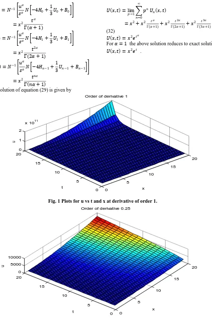
= 𝑥2+ 𝑥2_{Γ 𝛼+1} 𝑡𝛼 + 𝑥2_{Γ 2𝛼+1} 𝑡2𝛼 + 𝑥2_{Γ 3𝛼+1} 𝑡3𝛼 + ⋯ (32)

𝑈 𝑥, 𝑡 = 𝑥2_𝑒𝑡𝛼

For 𝛼 = 1 the above solution reduces to exact solution [25]

𝑈 𝑥, 𝑡 = 𝑥2_𝑒𝑡 _.

Fig. 1 Plots for u vs t and x at derivative of order 1.

Fig. 2 Plots for u vs t and x at derivative of order 0.25. 0

5

10

15

20

0 5

10 15

20 0 1 2

x 1011

x Order of derivative 1

t

u

0

5

10

15

20

0 5

10 15

20 0 5000 10000

x Order of derivative 0.25

t

International Journal of Innovative Technology and Exploring Engineering (IJITEE) ISSN: 2278-3075,Volume-8 Issue-12, October, 2019

Fig. 3 Plots for u vs t and x at derivative of order 0.5.

Fig. 4 Plots for u vs t and x at derivative of order 0.75.

Fig. 5 Plots for Error of approximate solution. 0

5

10

15

20

0 5

10 15

20 0 2 4

x 104

x Order of derivative 0.5

t

u

0

5

10

15

20

0 5

10 15

20 0 1 2

x 105

x Order of derivative 0.75

t

u

0

0.5

1

1.5

0 0.2

0.4 0.6

0.8 1

0 0.1 0.2

x

Error diagram of Numerical Solution up to III approximation with Exact Solution

t

Er

ro

5.1 Approximate third order solution of Fokker Planck for differential values of 𝜶 and absolute error

Table 5.1

Approximate third order solution of Fokker Planck for differential values of 𝛼 and absolute error at 𝛼 = 1.

Third order Approximate solution by HPNT Exact Error

T x 𝛼

= 0.5 𝛼 = 0.75

𝛼 = 1 𝛼 = 1 𝑈𝑒𝑥𝑎𝑐𝑡

− 𝑈𝐻𝑃𝑁𝑇

0.2

0.3 0.1375 0.1215 0.109 0.1099 2 × 10−4 0.6 0.5499 0.4861 0.4394 0.4397 3 × 10−4 0.8 0.9777 0.8642 0.7813 0.7817 4 × 10−4 0.4

0.3 0.1636 0.1491 0.1342 0.1343 1 × 10−4 0.6 0.6544 0.5963 0.5366 0.5371 5 × 10−4 0.8 1.1633 1.0601 0.9540 0.9548 8 × 10−4

VI. CONCLUSION

In the present work, we introduce a blend of Natural transform and homotopy perturbation method. We explored the methodology for the construction of the new twisting scheme and employed to compute the analytic approximate solution of a fractional-order non-linear Fokker Planck equation. By comparing these approximate solutions with known exact solutions, it was shown that the proposed solution is rapidly convergent with highaccuracywhich is shown by depiction of graphs and error analysis.

REFERENCES

1. B.J. West, M. Bolognab and P. Grigolini. Physics of Fractal Operators, Springer, New York. 2003.

2. M. Caputo. Linear models of dissipation whose q is almost frequency independent, part ii, J. Roy. Astr. Soc.(13) 529, 1976.

3. Podlubny, Fractional differential equations. An introduction to fractional derivatives fractional differential equations some methods of their solution and some of their applications, Academic Press, San Diego. 1999.

4. K.S. Miller and B. Ross, An Introduction to the Fractional Calculus and Fractional Differential Equations, Wiley-Interscience,New York,384. 1993.

5. S.G. Samko, A.A. Kilbas and O.I. Marichev, Integrals and Derivatives: Theory and Applications, Gordon and Breach, Yverdo. 1993.

6. J. Singh, D. Kumar and A. Kiliman, Numerical Solutions of Nonlinear Fractional Partial Differential Equations Arising in Spatial Diffusion of Biological Populations, Abstract and Applied Analysis. Volume 2014, Article ID 535793, 12 (2014).

7. D. Kumar, J. Singh and S. Kumar, Analytic and Approximate Solutions of Space-Time Fractional Telegraph Equations via Laplace Transform, Walailak Journal of Science and Technology. 11 (8), 711- 728 (2014).

8. S. Momani and Z. Odibat, Numerical comparison of methods for solving linear differential equations of fractional order, Chaos, Solitons and Fractals. 31(5), 1248-1255 (2007).

9. N.T. Shawagfeh, Analytical approximate solutions for nonlinear fractional differential equations, Applied Mathematics and Computation.131 (2-3), 517-529 (2002).

10. G. Oturan, A. Kurnaz and Y. Keskin, A new analytical approximate method for the solution of fractional differential equation, International Journal of Computer Mathematics 85 (1), 131-142 (2008).

11. A.S. Bataineh, A.K. Alomari, M.S.M. Noorani and I. Hashim, R. Nazar, Series Solutions of Systems of Nonlinear Fractional Differential Equations, Acta Appl Math. (105), 189-198 (2009). 12. Y. Khan and Q. Wu, Homotopy perturbation transform method for

non- linear equations using He’s polynomials, Computer and Mathematics with Applications. 61(8), 1963-1967 (2011).

13. J. Singh and D. Kumar, Homotopy perturbation algorithm using Laplace transform for gas dynamics equation, Journal of the Applied Mathematics, Statistics and Informatics. 8(1), 55-61 (2012).

14. J. Singh, D. Kumar and S. Rathore, Application of homotopy perturbation transform method for solving linear and nonlinear Klein-Gordon equations, Journal of Information and Computing Science. 7 (2) 131-139 (2012).

15. M.M. Khader and S. Kumar and S. Abbas bandy. New homotopy analysis transform method for solving the discontinued problems arising in Nano-technology, Chin Phys. B. 22(11) 110-201 (2013). 16. Silambarasan, R. and Belgacem, F.B.M. Theory of Natural

Transform. Mathematics in Engineering, Science and Aerospace (MESA), 3, 99-124(2012).

17. K. Yasir and F. Naeem, A new approach to differential difference equations, Journal of Advanced Research in Differential Equations. (2), 1-12 (2010).

18. Baskonus, H.M., Bulut, H. and Pandir, Y. The Natural Transform Decomposition Method for Linear. Mathematicsin Engineering, Science and Aerospace (MESA), 5, 111-126(2014).

19. Z.H.Khan andW.A.Khan.N-transform properties and applications. NUST Jour of Engg. Sciences.Vol. 1 No.1,pp. 127-133 (2008). 20. M.R.Spiegel.Theory and Problems of Laplace Transforms. Schaums

Outline Series,McGraw-Hill,New York,1965.

21. L.Debnath and D.Bhatta.Integral Transforms and their applications. 2nd edition.C.R.C.Press.London.2007.

22. Joel.L.Schiff.Laplace transform Theory and Applications. Auckland, New-Zealand. Springer 2005.

23. F.B.M.Belgacem,A.A.Karaballi and S.L.Kalla.Analytical investigations of the Sumudu transform and applications to integral production equations, Mathematical Problems in Engineering, no. 3, pp. 103-118(2003).

24. F.B.M.Belgacem and A.A.Karaballi.Sumudu transform fundamental properties investigations and applications. Journal of Applied Mathematics and Stochastic Analysis.Article ID 91083, pp.1-23 (2006).