Calculus
Know-It-ALL
Beginner to Advanced,
and Everything in Between
Stan Gibilisco
New York Chicago San Francisco Lisbon London Madrid Mexico City Milan New Delhi San Juan Seoul
database or retrieval system, without the prior written permission of the publisher. ISBN: 978-0-07-154932-5
MHID: 0-07-154932-3
The material in this eBook also appears in the print version of this title: ISBN: 978-0-07-154931-8, MHID: 0-07-154931-5. All trademarks are trademarks of their respective owners. Rather than put a trademark symbol after every occurrence of a trademarked name, we use names in an editorial fashion only, and to the benefit of the trademark owner, with no intention of infringement of the trademark. Where such designations appear in this book, they have been printed with initial caps.
McGraw-Hill eBooks are available at special quantity discounts to use as premiums and sales promotions, or for use in corporate training programs. To contact a representative please visit the Contact Us page at www.mhprofessional.com. Information contained in this work has been obtained by The McGraw-Hill Companies, Inc. (“McGraw-Hill”) from sources believed to be reliable. However, neither McGraw-Hill nor its authors guarantee the accuracy or completeness of any information published herein, and neither McGraw-Hill nor its authors shall be responsible for any errors, omissions, or damages arising out of use of this information. This work is published with the understanding that McGraw-Hill and its authors are supplying information but are not attempting to render engineering or other professional services. If such services are required, the assistance of an appropriate professional should be sought.
TERMS OF USE
This is a copyrighted work and The McGraw-Hill Companies, Inc. (“McGraw-Hill”) and its licensors reserve all rights in and to the work. Use of this work is subject to these terms. Except as permitted under the Copyright Act of 1976 and the right to store and retrieve one copy of the work, you may not decompile, disassemble, reverse engineer, reproduce, modify, create derivative works based upon, transmit, distribute, disseminate, sell, publish or sublicense the work or any part of it without McGraw-Hill’s prior consent. You may use the work for your own noncommercial and personal use; any other use of the work is strictly prohibited. Your right to use the work may be terminated if you fail to comply with these terms.
vii
About the Author
Preface xv
Acknowledgment xvii
Part 1 Differentiation in One Variable
1 Single-Variable Functions 3
Mappings 3
Linear Functions 9
Nonlinear Functions 12
“Broken” Functions 14
Practice Exercises 17
2 Limits and Continuity 20
Concept of the Limit 20
Continuity at a Point 24
Continuity of a Function 29
Practice Exercises 33
3 What’s a Derivative? 35
Vanishing Increments 35
Basic Linear Functions 40
Basic Quadratic Functions 44
Basic Cubic Functions 48
Practice Exercises 52
ix
Contents
4 Derivatives Don’t Always Exist 55
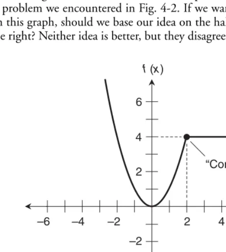
Let’s Look at the Graph 55
When We Can Differentiate 59
When We Can’t Differentiate 63
Practice Exercises 69
5 Differentiating Polynomial Functions 71
Power Rule 71
Sum Rule 75
Summing the Powers 79
Practice Exercises 82
6 More Rules for Differentiation 84
Multiplication-by-Constant Rule 84
Product Rule 87
Reciprocal Rule 90
Quotient Rule 95
Chain Rule 99
Practice Exercises 103
7 A Few More Derivatives 106
Real-Power Rule 106
Sine and Cosine Functions 108
Natural Exponential Function 114
Natural Logarithm Function 118
Practice Exercises 124
8 Higher Derivatives 126
Second Derivative 126
Third Derivative 130
Beyond the Third Derivative 133
Practice Exercises 136
9 Analyzing Graphs with Derivatives 138
Three Common Traits 138
Graph of a Quadratic Function 141
Graph of a Cubic Function 144
Graph of the Sine Function 147
Practice Exercises 152
Contents xi
Part 2 Integration in One Variable
11 What’s an Integral? 189
Summation Notation 189
Area Defined by a Curve 191
Three Applications 198
Practice Exercises 203
12 Derivatives in Reverse 205
Concept of the Antiderivative 205
Some Simple Antiderivatives 207
Indefinite Integral 211
Definite Integral 215
Practice Exercises 218
13 Three Rules for Integration 221
Reversal Rule 221
Split-Interval Rule 224
Substitution Rule 229
Practice Exercises 232
14 Improper Integrals 234
Variable Bounds 234
Singularity in the Interval 238
Infinite Intervals 244
Practice Exercises 248
15 Integrating Polynomial Functions 250
Three Rules Revisited 250
Indefinite-Integral Situations 253
Definite-Integral Situations 255
Practice Exercises 260
16 Areas between Graphs 262
Line and Curve 262
Two Curves 267
Singular Curves 270
Practice Exercises 274
17 A Few More Integrals 277
Sine and Cosine Functions 277
Natural Exponential Function 282
Reciprocal Function 289
18 How Long Is the Arc? 297
A Chorus of Chords 297
A Monomial Curve 302
A More Exotic Curve 306
Practice Exercises 309
19 Special Integration Tricks 311
Principle of Linearity 311
Integration by Parts 313
Partial Fractions 318
Practice Exercises 323
20 Review Questions and Answers 325
Part 3 Advanced Topics
21 Differentiating Inverse Functions 377
A General Formula 377
Derivative of the Arcsine 381
Derivative of the Arccosine 384
Practice Exercises 388
22 Implicit Differentiation 390
Two-Way Relations 390
Two-Way Derivatives 394
Practice Exercises 402
23 The L’Hôpital Principles 404
Expressions That Tend Toward 0/0 404
Expressions That Tend Toward ± ∞ /± ∞ 408
Other Indeterminate Limits 411
Practice Exercises 414
24 Partial Derivatives 416
Multi-Variable Functions 416
Two Independent Variables 419
Three Independent Variables 424
Practice Exercises 426
25 Second Partial Derivatives 428
Two Variables, Second Partials 428
Contents xiii
Three Variables, Second Partials 434
Three Variables, Mixed Partials 438
Practice Exercises 440
26 Surface-Area and Volume Integrals 442
A Cylinder 442
A Cone 444
A Sphere 448
Practice Exercises 453
27 Repeated, Double, and Iterated Integrals 455
Repeated Integrals in One Variable 455
Double Integrals in Two Variables 458
Iterated Integrals in Two Variables 462
Practice Exercises 466
28 More Volume Integrals 468
Slicing and Integrating 468
Base Bounded by Curve and x Axis 470
Base Bounded by Curve and Line 475
Base Bounded by Two Curves 481
Practice Exercises 487
29 What’s a Differential Equation? 490
Elementary First-Order ODEs 490
Elementary Second-Order ODEs 493
Practice Exercises 500
30 Review Questions and Answers 502
Final Exam 541
Appendix A Worked-Out Solutions to Exercises: Chapters 1 to 9 589
Appendix B Worked-Out Solutions to Exercises: Chapters 11 to 19 631
Appendix C Worked-Out Solutions to Exercises: Chapters 21 to 29 709
Appendix D Answers to Final Exam Questions 775
Appendix E Special Characters in Order of Appearance 776
Appendix G Table of Integrals 779
Suggested Additional Reading 783
xv
Preface
If you want to improve your understanding of calculus, then this book is for you. It can sup-plement standard texts at the high-school senior, trade-school, and college undergraduate levels. It can also serve as a self-teaching or home-schooling supplement. Prerequisites include intermediate algebra, geometry, and trigonometry. It will help if you’ve had some precalculus (sometimes called “analysis”) as well.
This book contains three major sections. Part 1 involves differentiation in one variable. Part 2 is devoted to integration in one variable. Part 3 deals with partial differentiation and multiple integration. You’ll also get a taste of elementary differential equations.
Chapters 1 through 9, 11 through 19, and 21 through 29 end with practice exercises. You may (and should) refer to the text as you solve these problems. Worked-out solutions appear in Apps. A, B, and C. Often, these solutions do not represent the only way a problem can be figured out. Feel free to try alternatives!
Chapters 10, 20, and 30 contain question-and-answer sets that finish up Parts 1, 2, and 3, respectively. These chapters will help you review the material.
A multiple-choice final exam concludes the course. Don’t refer to the text while taking the exam. The questions in the exam are more general (and easier) than the practice exercises at the ends of the chapters. The exam is designed to test your grasp of the concepts, not to see how well you can execute calculations. The correct answers are listed in App. D.
In my opinion, most textbooks place too much importance on “churning out answers,” and often fail to explain how and why you get those answers. I wrote this book to address these problems. I’ve tried to introduce the language gently, so you won’t get lost in a wilderness of jargon. Many of the examples and problems are easy, some take work, and a few are designed to make you think hard.
If you complete one chapter per week, you’ll get through this course in a school year. But don’t hurry. When you’ve finished this book, I recommend Calculus Demystified by Steven G. Krantz and Advanced Calculus Demystified by David Bachman for further study. If Chap. 29 of this book gets you interested in differential equations, I recommend Differential Equations Demystified by Steven G. Krantz as a first text in that subject.
xvii
Acknowledgment
1
PART
1
Calculus is the mathematics of functions, which are relationships between sets consisting of objects called elements. The simplest type of function is a single-variable function, where the elements of two sets are paired off according to certain rules.
Mappings
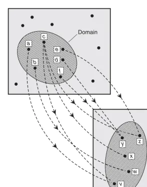
Imagine two sets of points defined by the large rectangles in Fig. 1-1. Suppose you’re inter-ested in the subsets shown by the hatched ovals. You want to pair off the points in the top oval with those in the bottom oval. When you do this, you create a mapping of the elements of one set into the elements of the other set.
Domain, range, and variables
All the points involved in the mapping of Fig. 1-1 are inside the ovals. The top oval is called thedomain. That’s the set of elements that we “go out from.” In Fig. 1-1, these elements are a through f. The bottom oval is called the range. That’s the set of elements that we “come in toward.” In Fig. 1-1, these elements are v through z.
In any mapping, the elements of the domain and the range can be represented by vari-ables. A nonspecific element of the domain is called the independent variable. A nonspecific element of the range is called the dependent variable. The mapping assigns values of the depen-dent (or “output”) variable to values of the independepen-dent (or “input”) variable.
Ordered pairs
In Fig. 1-1, the mapping can be defined in terms of ordered pairs, which are two-item lists showing how the elements are assigned to each other. The set of ordered pairs defined by the mapping in Fig. 1-1 is
{(a,v), (b,w), (c,v), (c,x), (c,z), (d,y), (e,z), ( f,y)}
3
CHAPTER
1
Within each ordered pair, an element of the domain (a value of the independent variable) is written before the comma, and an element of the range (a value of the dependent variable) is written after the comma. Whenever you can express a mapping as a set of ordered pairs, then that mapping is called a relation.
Are you confused?
You won’t see spaces after the commas inside of the ordered pairs, but you’ll see spaces after the commas separating the ordered pairs in the list that make up the set. These aren’t typographical errors! That’s the way they should be written.
Range
a b
c
d e
v w x y z f
[image:25.546.106.399.54.425.2]Domain
Modifying a relation
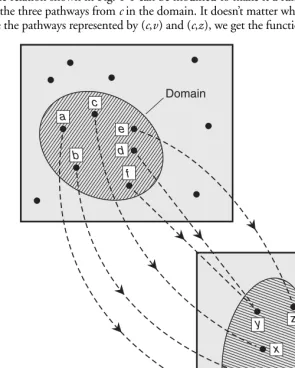
Afunction is a relation in which every element in the domain maps to one, but never more than one, element in the range. This is not true of the relation shown in Fig. 1-1. Element c in the domain maps to three different elements in the range: v,x, and z.
In a function, it’s okay for two or more values of the independent variable to map to a single value of the independent variable. But it is not okay for a single value of the indepen-dent variable to map to two or more values of the depenindepen-dent variable. A function can be many-to-one, but never one-to-many. Sometimes, in order to emphasize the fact that no value of the independent variable maps into more than one value of the dependent variable, we’ll talk about this type of relation as a true function or a legitimate function.
The relation shown in Fig. 1-1 can be modified to make it a function. We must eliminate two of the three pathways from c in the domain. It doesn’t matter which two we take out. If we remove the pathways represented by (c,v) and (c,z), we get the function illustrated in Fig. 1-2.
Mappings 5
Range
a b
c
d e
v w x y z f
[image:26.568.106.401.228.596.2]Domain
Here’s an informal way to think of the difference between a relation and a function. A rela-tion correlates things in the domain with things in the range. A funcrela-tion operates on things in the domain to produce things in the range. A relation merely sits there. A function does something!
Three physical examples
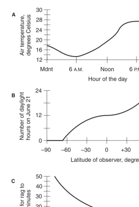
Let’s look at three situations that we might encounter in science. All three of the graphs in Fig. 1-3 represent functions. The changes in the value of the independent variable can be thought of as causative, or at least contributing, factors that affect the value of the dependent variable. We can describe these situations as follows:
• The outdoor air temperature is a function of the time of day.
• The number of daylight hours on June 21 is a function of latitude.
• The time required for a wet rag to dry is a function of the air temperature.
A mathematical example
Imagine a relation in which the independent variable is called x and the dependent variable is calledy, and for which the domain and range are both the entire set of real numbers (also called thereals). Our relation is defined as
y=x+ 1
This is a function between x and y, because there’s never more than one value of y for any value ofx. Mathematicians name functions by giving them letters of the alphabet such as f, g, and h. In this notation, the dependent variable is replaced by the function letter followed by the independent variable in parentheses. We can write
f (x)=x+ 1
to represent the above equation, and then we can say, “f of x equals x plus 1.” When we write a function this way, the quantity inside the parentheses (in this case x) is called the argument of the function.
The inverse of a relation
We can transpose the domain and the range of any relation to get its inverse relation, also called simply the inverse if the context is clear. The inverse of a relation is denoted by writing a superscript −1 after the name of the relation. It looks like an exponent, but it isn’t meant to be.
The inverse of a relation is always another relation. But when we transpose the domain and range of a function, we don’t always get another true function. If we do, then the function and its inverse reverse, or “undo,” each other’s work.
Suppose that x and y are variables, f and f −1 are functions that are inverses of each other,
and we know these two facts:
f (x)=y and
Then the following two facts are also true:
f −1 [ f (x)]= x
and
f [ f −1 ( y)]=y Hour of the day
Air temper
ature
,
deg
rees Celsius
Mdnt 6A.M. Noon 6P.M. Mdnt
12 16 20 24 28 30 Time f or r ag to dr y, min utes
Air temperature, degrees Celsius
10 20 30
0 10 20 30 40
15 25 35
Latitude of observer, degrees
50
0 –30 –60
–90 +30 +60 +90
0 12 24 A B C
Number of da
ylight
hours on J
[image:28.568.109.393.60.482.2]une 21
Figure 1-3 At A, the air temperature is a function of the time of day. At B, the number of daylight hours on June 21 is a function of the latitude (positive is north; negative is south). At C, the drying time for a wet rag is a function of the air temperature.
Are you confused?
It’s reasonable to wonder, “Can we tell whether or not a relation is a function by looking at its graph?” The answer is yes. Consider a graph in which the independent variable is represented by the horizontal axis, and the dependent variable is represented by the vertical axis. Imagine a straight, vertical line extending infinitely upward and downward. We move this vertical line to the left and right, so the point where it intersects the independent-variable axis sweeps through every possible argument of the relation. A graph represents a function “if and only if” that graph never crosses a movable vertical line at more than one point. Let’s call this method of graph-checking thevertical-line test.
Here’s a note!
In mathematics, the expression “if and only if” means that logical implication works in both direc-tions. In the above example, we are really saying two things:
• If a graph represents a function, then the graph never crosses a movable vertical line at more than one point.
• If a graph never crosses a movable vertical line at more than one point, then the graph repre-sents a function.
The expression “if and only if” is abbreviated in text as “iff.” In logic, it’s symbolized by a double-shafted, double-headed arrow pointing to the left and right (⇔).
Here’s a challenge!
Imagine that the independent and dependent variables of the functions shown in Fig. 1-3 are reversed. This gives us some weird assertions.
• The time of day is a function of the outdoor air temperature.
• Latitude is a function of the number of daylight hours on June 21.
• The air temperature is a function of the time it takes for a wet rag to dry.
Only one of these statements translates into a mathematical function. Which one?
Solution
You can test the graph of a relation to see if its inverse is a function by doing a horizontal-line test. It works like the vertical-line test, but the line is parallel to the independent-variable axis, and it moves up and down instead of to the left and right. The inverse of a relation represents a function if and only if the graph of the original relation never intersects a movable horizontal line at more than one point.
Linear Functions
When the argument changes in a linear function, the value of the dependent variable changes in constant proportion. That proportion can be positive or negative. It can even be zero, in which case we have a constant function.
Slope and intercept
In conventional coordinates, linear functions always produce straight-line graphs. Conversely, any straight line represents a linear function, as long as that line isn’t parallel to the dependent-variable axis.
Theslope, also called the gradient, of a straight line in rectangular coordinates (where the axes are perpendicular to each other and the divisions on each axis are of uniform size) is an expres-sion of the steepness with which the line goes upward or downward as we move to the right. A horizontal line, representing a constant function, has a slope of zero. A line that ramps upward as we move to the right has positive slope. A line that ramps downward as we move to the right has negative slope. Figure 1-4 shows a line with positive slope and another line with negative slope.
To calculate the slope of a line, we must know the coordinates of two points on that line. If we call the independent variable x and the dependent variable y, then the slope of a line, passing through two points, is equal to the difference in the y-values divided by the difference in the x-values. We abbreviate “the difference in” by writing the uppercase Greek letter delta (Δ). Let’s use a to symbolize the slope. Then
a= Δy/Δx
2 4 6
–6
2 4 6
–2
–4
–6
x y
–4 –2
y-intercept is 3
y-intercept is –2 Slope is
negative Slope is positive
Figure 1-4 Graphs of two linear functions.
We read this as “delta y over delta x.” Sometimes the slope of a straight line is called rise over run. This makes sense as long as the independent variable is on the horizontal axis, the depen-dent variable is on the vertical axis, and we move to the right.
Anintercept is a point where a graph crosses an axis. We can plug 0 into a linear equation for one of the variables, and solve for the other variable to get its intercept. In a linear func-tion, the term y-intercept refers to the value of the dependent variable y at the point where the line crosses the y axis. In Fig. 1-4, the line with positive slope has a y-intercept of 3, and the line with negative slope has a y-intercept of −2.
Standard form for a linear function
If we call the dependent variable x, then the standard form for a linear function is f (x)=ax+b
where a and b are real-number constants, and f is the name of the function. As things work out,a is the slope of the function’s straight-line graph. If we call the dependent variable y, then b is the y-intercept. We can substitute y in the equation for f (x), writing
y=ax+b
Either of these two forms is okay, as long as we keep track of which variable is independent and which one is dependent!
Are you confused?
If the graph of a linear relation is a vertical line, then the slope is undefined, and the relation is not a function. The graph of a linear function can never be parallel to the dependent-variable axis (or perpendicular to the independent-variable axis). In that case, the graph fails the verti-cal-line test.
Here’s a challenge!
Rewrite the following equation as a linear function of x, and graph it on that basis:
12x+ 6y= 18
Solution
We must rearrange this equation to get y all by itself on the left side of the equals sign, and an expres-sion containing only x and one or more constants on the right side. Subtracting 12x from both sides gives us:
6y= −12x+ 18
Dividing each side by 6 puts it into the standard form for a linear function:
If we name the function f, then we can express the function as f (x)= −2x+ 3
In the graph of this function, the y-intercept is 3. We plot the y-intercept on the y axis at the mark for 3 units, as shown in Fig. 1-5. That gives us the point (0,3). To find the line, we must know the coordi-nates of one other point. Let’s find the x-intercept! To do that, we can plug in 0 for y to get
0= −2x+ 3
Adding 2x to each side and then dividing through by 2 tells us that x= 3/2. Therefore, the point (3/2,0) lies on the line. Now that we know (0,3) and (3/2,0) are both on the line, we can draw the line through them.
Here’s a twist!
When we move from (0,3) to (3/2,0) in Fig. 1-5, we travel in the negative y direction by 3 units, so
Δy= −3. We also move in the positive x direction by 3/2 units, so Δx= 3/2. Therefore
Δy/Δx= −3/(3/2) = −2
reflecting the fact that the slope of the line is −2. We’ll always get this same value for the slope, no matter which two points on the line we choose. Uniformity of slope is characteristic of all linear functions. But there are functions for which it isn’t so simple.
4 6
–6
2 6
–2
–4
–6
x y
–4 –2
Slope = –2
(0,3)
y-intercept is 3 (3/2,0)
x-intercept is 3/2
f(x) = –2x+ 3
y= –2x+ 3
Figure 1-5 Graph of the linear function y= −2x+ 3.
Nonlinear Functions
When the value of the argument changes in a nonlinear function, the value of the dependent variable also changes, but not always in the same proportion. The slope can’t be defined for the whole function, although the notion of slope can usually exist at individual points. In rectangular coordinates, the graph of a nonlinear function is always something other than a straight line.
Square the input
Let’s look at a simple nonlinear relation. The domain is the entire set of reals, and the range is the set of nonnegative reals. The equation is
y=x2
If we call the relation g, we can write
g (x)=x2
For every value of x in the domain of g, there is exactly one value of y in the range. Therefore, g is a function. But, as we can see by looking at the graph of g shown in Fig. 1-6, the reverse is not true. For every nonzero value of y in the range of g, there are two values of x in the domain. These two x-values are always negatives of each other. For example, if y= 49, then x= 7 or x= −7. This means that the inverse of g is not a function.
2 4 6
–2 –4 –6
2 6
–2
–4
–6
x y
4 Slope
varies
g(x) = x2 y=x2
Cube the input
Here’s another nonlinear relation. The domain and range both span the entire set of reals. The equation is
y=x3
This is a function. If we call it h, then:
h (x)=x3
For every value of x in the domain of h, there is exactly one value of y in the range. The reverse is also true. For every value of y in the range of h, there is exactly one x in the domain. This means that the inverse of h is also a function. We can see this by looking at the graph of h (Fig. 1-7). When a function is one-to-one and its inverse is also one-to-one, then the function is called a bijection.
Are you confused?
Have you noticed that in Fig. 1-7, the y axis is graduated differently than the x axis? There’s a reason for this. We want the graph to fit reasonably well on the page. It’s okay for the axes in a rectangular coordinate system to have increments of different sizes, as long as each axis maintains a constant increment size all along its length.
2 4 6
–2 –4 –6
x y
Slope varies 30
20
10
–10
–20
–30
y=x3
h(x) = x3
Figure 1-7 Graph of the nonlinear function y=x3.
Here’s a challenge!
Look again at the functions g and h described above, and graphed in Figs. 1-6 and 1-7. The inverse of
h is a function, but the inverse of g is not. Mathematically, demonstrate the reasons why.
Solution
Here’s the function g again. Remember that the domain is the entire set of reals, and the range is the set of nonnegative reals:
y =g (x)=x2
If you take the equation y=x2 and transpose the positions of the independent and dependent variables, you get
x=y2
This is the same as
y = ± (x1/2)
The plus-or-minus symbol indicates that for every value of the independent variable x you plug in you’ll get two values of y, one positive and the other negative. You can also write
g−1 (x)= ± (x1/2)
The function g is two-to-one (except when y= 0), and that’s okay. But the inverse relation is one-to-two (except when y= 0). So, while g−1 is a legitimate relation, it is not a function.
The function h has an inverse that is also a function. Remember from your algebra and set theory courses that the inverse of any bijection is also a bijection. You have
h (x)=x3
and
h−1 (x)=x1/3
If a function is one-to-one over a certain domain and range, then you can transpose the values of the independent and dependent variables while leaving their names the same, and you can also transpose the domain and range. That gives you the inverse, and it is a function. However, if a function is many-to-one, then its inverse is one-to-many, so that inverse is not a function.
“Broken” Functions
A three-part function
Figure 1-8 is a graph of a function where the value is −3 if the argument is negative, 0 if the argument is 0, and 3 if the argument is positive. Let’s call the function f. Then we can write
f(x)= −3 if x < 0 = 0 if x= 0 = 3 if x > 0
Even though this function takes two jumps, there are no gaps in the domain. The function is defined for every real number x.
The reciprocal function
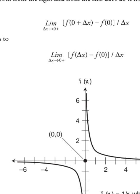
Figure 1-9 is a graph of the reciprocal function. We divide 1 by the argument. If we call this functiong, then we can write
g (x)= 1/x
This graph has a two-part blow-up at x= 0. As we approach 0 from the left, the graph blows up negatively. As we approach 0 from the right, it blows up positively. The function is defined for all values of x except 0.
2 4 6
–2 –4 –6
2 6
–2
–4
–6
x y
4
y= –3 if x< 0
y= 0 if x= 0
y= 3 if x> 0
Figure 1-8 Graph of the “broken” function y= −3 ifx < 0, y= 0 if x= 0, y= 3 if x > 0.
The tangent function
Figure 1-10 is a graph of the tangent function from trigonometry. If we call this function h, then we can write
h (x)= tan x
This graph blows up at infinitely many values of the independent variable! It is defined for all values of x except odd-integer multiples of p/2.
Are you confused?
Does it seem strange that a function can jump abruptly from one value to another, skip over individual points, or even blow up to “infinity” or “negative infinity”? You might find this idea difficult to com-prehend if you’re the literal-minded sort. But as long as a relation passes the test for a function accord-ing to the rules we’ve defined, it’s a legitimate function.
Here’s a challenge!
Draw a graph of the relation obtained by rounding off an argument to the nearest integer smaller than or equal to itself. Call the independent variable x and the dependent variable y. Here are some examples to give you the idea:
If x= 3, then y= 3
Ifx= −6, then y= −6
2 4 6
–2 –4 –6
2 6
–2
–4
–6
x y
4
y= 1/x
Ifx= π, then y= 3
Ifx= −π, then y= −4
Ifx= 4.999, then y= 4
If x= −5.001, then y= −6
Is the relation represented by this graph a function? How can we tell?
Solution
This graph is shown in Fig. 1-11. It passes the vertical-line test, so it represents a function. We can also tell that this relation is a function by the way it’s defined. No matter what the argument, the relation maps it to one, but only one, integer. This type of function is called a step function because of the way its graph looks.
Practice Exercises
This is an open-book quiz. You may (and should) refer to the text as you solve these problems. Don’t hurry! You’ll find worked-out answers in App. A. The solutions in the appendix may not
–3p
3p 3
2
1
y
x
–1
–2
–3
y= tan x
Figure 1-10 Graph of the “broken” function y= tan x.
represent the only way a problem can be figured out. If you think you can solve a particular problem in a quicker or better way than you see there, by all means try it!
1. Imagine a mapping from the set of all integers onto the set of all nonnegative integers in which the set of ordered pairs is
{(0,0), (1,1), (−1,2), (2,3), (−2,4), (3,5), (−3,6), (4,7), (−4,8), . . . }
Is this relation a function? If so, why? If not, why not? Is its inverse a function? If so, why? If not, why not?
2. Consider a mapping from the set of all integers onto the set of all nonnegative integers in which the set of ordered pairs is
{(0,0), (1,1), (−1,1), (2,2), (−2,2), (3,3), (−3,3), (4,4), (−4,4), . . . }
Is this relation a function? If so, why? If not, why not? Is its inverse a function? If so, why? If not, why not?
3. Consider the following linear function:
f (x)= 4x − 5 What is the inverse of this? Is it a function?
x y
6
4
2
–4
–6
–6 –4 –2 2 4 6
4. Consider the following linear function: g (x)= 7
What is the inverse of this? Is it a function?
5. In the Cartesian coordinate xy plane, the equation of a circle with radius 1, centered at the origin (0,0), is
x2+y2= 1
This particular circle is called the unit circle. Is its equation a function of x? If so, why? If not, why not?
6. Is the equation of the unit circle, as expressed in Prob. 5, a function of y? If so, why? If not, why not?
7. Consider the nonlinear function we graphed in Fig. 1-6: g (x)=x2
As we saw, the inverse relation, g−1, is not a function. But it can be modified so it
becomes a function of x by restricting its range to the set of positive real numbers. Show with the help of a graph why this is true. Does g−1 remain a function if we
allow the range to include 0?
8. We can modify the relation g−1 from the previous problem, making it into a function
ofx, by restricting its range to the set of negative real numbers. Show with the help of a graph why this is true. Does g−1 remain a function if we allow the range to
include 0?
9. Look again at Figs. 1-8 through 1-10. All three of these graphs pass the vertical-line test for a function. This is true even though the relation shown in Fig. 1-9 is not defined when x= 0, and the relation shown in Fig. 1-10 is not defined when x is any odd-integer multiple of p/2. Now suppose that we don’t like the gaps in the domains in Figs. 1-9 and 1-10. We want to modify these functions to make their domains cover the entire set of real numbers. We decide to do this by setting y= 0 whenever we encounter a value of x for which either of these relations is not defined. Are the relations still functions after we do this to them?
10. Consider again the functions graphed in Figs. 1-8 through 1-10. The inverse of one of these functions is another function. That function also happens to be its own inverse. Which one of the three is this?
20
2
Limits and Continuity
While Isaac Newton and Gottfried Wilhelm Leibniz independently developed the differen-tial calculus in the seventeenth century, they both wanted to figure out how to calculate the instantaneous rate of change of a nonlinear function at a point in space or time, and then describe the rate of change in general, as a function itself. In the next few chapters, we’ll do these things. But first, let’s be sure we have all the mathematical tools we need!
Concept of the Limit
As the argument (the independent variable or input) of a function approaches a particular value, the dependent variable approaches some other value called the limit. The important word here is approaches. When finding a limit, we’re interested in what happens to the func-tion as the argument gets closer and closer to a certain value without actually reaching it.
Limit of an infinite sequence
Let’s look at an infinite sequence S that starts with 1 and then keeps getting smaller: S = 1, 1/2, 1/3, 1/4, 1/5, . . .
As we move along in S from term to term, we get closer and closer to 0, but we never get all the way there. If we choose some small positive number r, no matter how tiny, we can always find a number in S (if we’re willing to go out far enough) smaller than r but larger than 0. Because of this fact, we can say, “If n is a positive integer, then the limit of S, as n gets endlessly larger, is 0.” We write this symbolically as
Lim n→∞ S= 0
arbitrarily large.” This expression is a little bit obscure, because we can debate whether large numbers are really closer to “infinity” than small ones. But we’ll often hear that expression used, nevertheless.
When talking about this sequence S, we can also say, “The limit of 1/n, as n approaches infinity, is equal to 0,” and write
Lim
n→∞ 1/n= 0
Limit of a function
Now let’s think about what takes place if we don’t restrict ourselves to positive-integer argu-ments. Let’s consider the function
g (x)= 1/x
and allow x to be any positive real number. As x gets larger, g (x) gets smaller, approaching 0 but never getting there. We can say, “The limit of g (x), as x approaches infinity, is 0,” and write
Lim
n→∞ g (x)= 0
This is the same as the situation with the infinite sequence of positive integers, except that the function approaches 0 smoothly, rather than in jumps.
Are you a nitpicker?
Let’s state the above expression differently. For every positive real number r, there exists a positive real numbers such that
0 < g (s) < r
Also, if t is a real number larger than s, then
0 < g (t) < g (s) < r
Think about this language for awhile. It’s a formal way of saying that as we input larger and larger positive real numbers to the function g, we get smaller and smaller positive reals that “close in” on 0. This statement also tells us that even if we input huge numbers such as 1,000,000, 1,000,000,000, or 1,000,000,000,000 to the function g, we’ll never get 0 when we calculate g (x). We can’t input “infinity” in an attempt to get 0 out of g, either. “Infinity” isn’t a real number!
Are you confused?
If the notion of “closing in on 0” confuses you, look at the graph of the function g for large values of x. As you move out along the x axis in the positive direction, the curve gets closer and closer to the x axis, where
g (x)= 0. No matter how close the curve gets to the axis, you can always get it to come closer by moving out farther in the positive x direction, as shown in Fig. 2-1. But the curve never reaches the x axis.
Sum rule for two limits
Consider two functions f (x) and g (x) with different limits. We can add the functions and take the limit of their sum, and we’ll get the same thing as we do if we take the limits of the functions separately and then add them. Let’s call this the sum rule for two limits and write it symbolically as
Lim
x→k [ f (x)+g (x)] = Limx→k f (x)+ Limx→k g (x)
where k, the value that x approaches, can be a real-number constant, another variable, or “infinity.” This rule isn’t restricted to functions. It holds for any two expressions with defin-able limits. It also works for the difference between two expressions. We can write
Lim
x→k [ f (x) − g (x)] = Limx→k f (x) − Limx→k g (x) g(x)
g(x) = 1/x
x
x
x
Axis Curve
Keep
going
Keep
going
Magnify
Figure 2-1 As x increases endlessly, the value of 1/x
In verbal terms, we can say these two things:
• The limit of the sum of two expressions is equal to the sum of the limits of the expressions. • The limit of the difference between two expressions is equal to the difference between
the limits of the expressions (in the same order).
Multiplication-by-constant rule for a limit
Now consider a function with a defined limit. We can multiply that limit by a constant, and we’ll get the same thing as we do if we multiply the function by the constant and then take the limit. Let’s call this the multiplication-by-constant rule for a limit. We write it symbolically as
c Limx→k f (x)=Limx→k c [ f (x)]
where c is a real-number constant, and k is, as before, a real-number constant, another vari-able, or “infinity.” As with the sum rule, this holds for any expressions with definable limits, not only for functions. In verbal terms, we can say this:
• A constant times the limit of an expression is equal to the limit of the expression times the constant.
Here’s a challenge!
Determine the limit, as x approaches 0, of a function h (x) that raises x to the fourth power and then takes the reciprocal:
h (x)= 1/x4 Symbolically, this is written as
Lim x→0 1/x4
Solution
Asx starts out either positive or negative and approaches 0, the value of 1/x4 increases endlessly. No matter how
large a number you choose for h (x), you can always find something larger by inputting some x whose absolute value is small enough. In this situation, the limit does not exist. You can also say that it’s not defined.
Once in awhile, someone will write the “infinity” symbol, perhaps with a plus sign or a minus sign in front of it, to indicate that a limit blows up (increases without bound) positively or negatively. For example, the solution to this “challenge” could be written as
Lim x→0 1/x
4= ∞
or as
Lim x→0 1/x
4= + ∞
Continuity at a Point
When we scrutinize a function or its graph, we might want to talk about its continuity at a point. But first, we must know the value of the function at that point, as well as the limit as we approach it from either direction.
Right-hand limit at a point
Consider the following function, which takes the reciprocal of the input value: g (x)= 1/x
We can’t define the limit of g (x) as x approaches 0 from the positive direction, because the function blows up as x gets smaller positively, approaching 0. To specify that we approach 0 from the positive direction, we can refine the limit notation by placing a plus sign after the 0, like this:
Lim x→ +0 g (x)
This expression reads, “The limit of g (x) as x approaches 0 from the positive direction.” We can also say, “The limit of g (x) as x approaches 0 from the right.” (In most graphs where x is on the horizontal axis, the value of x becomes more positive as we move toward the right.) This sort of limit is called a right-hand limit.
Right-hand continuity at a point
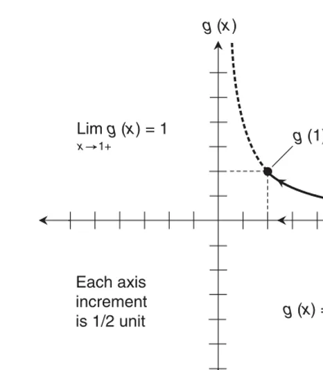
What about some other point, such as where x = 1? As we approach the point where x = 1 from the positive direction, g starts out at positive values smaller than 1 and increases, approaching 1. We can see this with the help of Fig. 2-2, which is a graph of g drawn in the vicinity of the point where x = 1. (Each division on the axes represents 1/2 unit.) This graph tells us that
Lim
x→1+ g (x)= 1 We can calculate the actual value of g for x = 1, getting
g (1) = 1/1 = 1
Now suppose that:
• We can define the right-hand limit of a function at a certain point • We can define the actual value of the function at that point • The limit and the actual value are the same
Left-hand limit at a point
Let’s expand the domain of g to the entire set of reals except 0, for which g is not defined because 1/0 is not defined. Suppose that we start out with negative real values of x and approach 0 from the left. As we do this, g decreases endlessly, as we can see by looking at Fig. 2-3. (Here, each division on the axes represents 1 unit.) Another way of saying this is that g increases negatively without limit, or that it blows up negatively. Therefore,
Lim x→ −0 g (x)
is not defined. We read the above symbolic expression as, “The limit of g (x) as x approaches 0 from the negative direction.” We can also say, “The limit of g (x) as x approaches 0 from the left.” This sort of limit is called a left-hand limit.
Left-hand continuity at a point
Now let’s look again at the point in the graph g where x= 1. Suppose we approach this point from the left, that is, from the negative direction. The value of g starts out at positive values larger than 1. As x increases and approaches 1, g decreases, getting closer and closer to 1. Figure 2-4 illustrates what happens here. (Each division on the axes represents 1/2 unit.) We have
Lim
x→ −1 g (x)= 1
Each axis increment is 1/2 unit
g(1) = 1 Limg(x) = 1
x 1+
x g(x)
[image:46.568.137.370.62.329.2]g(x) = 1/x
Figure 2-2 The limit of the function g (x) = 1/x as x
approaches 1 from the right is equal to the value of the function when x = 1. In this graph, each axis division represents 1/2 unit.
x
Limg(x)
x 0–
is not defined Each axis increment is 1 unit
g(x)
g(x) = 1/x
Figure 2-3 As x approaches 0 from the negative direction, the value of 1/x increases negatively without limit. In this graph, each axis division represents 1 unit.
Each axis increment is 1/2 unit
g(1) = 1
g(x) = 1/x
x g(x)
Limg(x) = 1
x 1–
Figure 2-4 The limit of the function g (x) = 1/x as x
We already know that g (1) = 1. Just as we did when approaching from the right, we can say thatg is left-hand continuous at the point where x = 1. Some texts will say that g is continuous on the left at that point.
Are you confused?
It’s easy to get mixed up by the meanings of “negative direction” and “positive direction,” and how these relate to the notions of “left-hand” and “right-hand.” These terms are based on the assumption that we’re talking about the horizontal axis in a graph, and that this axis represents the independent variable. In most graphs of this type, the value of the independent variable gets more negative as we move to the left, and more positive as we move to the right. This is true no matter where on the axis we start.
As we travel along the horizontal axis, we might be in positive territory the whole time; we might be in negative territory the whole time; we might cross over from the negative side to the positive side or vice-versa. Whenever we come toward a point from the left, we approach from the negative direction, even if that point corresponds to something like x = 567. Whenever we come toward a point from the right, we approach from the positive direction, even if the point is at x =−53,535. The location of the point doesn’t matter. The important thing is the direction from which we approach.
“Total” continuity at a point
Now that we’ve defined right-hand and left-hand continuity at a point, we can define conti-nuity at a point in a “total” sense. When a function is both left-hand continuous and right-hand continuous at a point, we say that the function is continuous at that point. Conversely, whenever we say that a function is continuous at a point, we mean that it’s continuous as we approach and then reach the point from both the left-hand side and the right-hand side.
Here’s a challenge!
Suppose we modify the function g (x) = 1/x by changing the value for x= 1. Let’s call this new function
g∗. The domain remains the same: all real numbers except 0. The only difference between g∗ and g is that
g∗ (1) is not equal to 1, but instead is equal to 4, as shown in Fig. 2-5. (In this graph, each axis division is 1 unit.) We have seen that the original function g is both right-hand continuous and left-hand continuous at (1,1), so we know that g is “totally” continuous at (1,1). But what about g∗? Is this modified function continuous at the point where x= 1? Is it left-hand continuous there? Is it right-hand continuous there?
Solution
The answer to each of these three questions is “No.” The function g∗ is not continuous at the point where
x= 1. It’s not right-hand continuous or left-hand continuous there. The limit of g∗ as we approach x= 1 from either direction is equal to 1. That is,
Lim
x→ +1 g∗ (x)= 1
and
Lim
x→ −1 g∗ (x)= 1
As we move toward the point where x= 1 from either direction along the curve, it seems as if we should end up at the point (1,1) when the value of x reaches 1. But when we look at the actual value of g∗ at x= 1, we find that it’s not equal to 1. There is a discontinuity in g∗ at the point where x= 1. We can also say that
g∗ is not continuous at the point where x= 1, or that g∗ is discontinuous at the point where x= 1.
Here’s another challenge!
Look again at the step function we saw in Fig. 1-11 near the end of Chap. 1. Is this function right-hand continuous at point where x= 3? Is it left-hand continuous at that point?
Solution
A portion of that function is reproduced in Fig. 2-6, showing only the values in the vicinity of our point of interest. Let’s call the function s (x). We can see from this drawing that
Lim
x→ +3 s (x)= 3
x
Each axis increment is 1 unit
g(x)
(1,4)
g* (x) = 1/xwhenx≠ 1 = 4 when x= 1
Figure 2-5 A modified function g∗, which is the same as
and
Lim
x→ −3 s (x)= 2
The value of the function at the point where x= 3 is s (3) = 3. The right-hand limit and the actual value are the same, so s is right-hand continuous at the point where x= 3. But s is not left-hand continuous at the point where x= 3, because the left-hand limit and the actual value are different. The same situation occurs at every integer value of x in the step function illustrated in Fig. 1-11. Because s is not continuous from both the right and the left at any point where x is an integer, s is not continuous at any such point. This function has an infinite number of discontinuities!
Continuity of a Function
A real-number function in one variable is a continuous function if and only if it is continuous at every point in its domain. Imagine a line or curve that’s smooth everywhere, with no gaps, no jumps, and no blow-ups in its domain. That’s what a continuous function looks like when graphed.
Linear functions
Alllinear functions are continuous. A real-number linear function L always has an equation of this form:
L (x)=ax+b
Lims(x) = 2
x 3 –
Lims(x) = 3
x 3 +
x
6
4
2
2 4 6
s(x)
Figure 2-6 Limits of a step function,
s (x), at the point where x = 3.
where x is the independent variable, a is a nonzero real number, and b can be any real number. In rectangular coordinates, the graph of a linear function is a straight line that extends forever in two opposite directions. It never has a discontinuity.
Figure 2-7 shows four generic graphs of linear functions. The independent variable is on the horizontal axis, and the dependent variable is on the vertical axis.
Quadratic functions
All single-variable, real-number quadratic functions are continuous. The general form of a quadratic function Q is
Q (x)=ax2+bx+c
where x is the independent variable, a is a nonzero real, and b and c can be any reals. In rect-angular coordinates, the graph of a quadratic function is always a parabola that opens either straight up or straight down. The domain includes all reals, but the range is restricted to either the set of all reals greater than or equal to a certain absolute minimum, or the set of all reals less than or equal to a certain absolute maximum. There are never any gaps, jumps, or blow-ups in the graph within the domain.
Figure 2-8 shows four generic graphs of quadratic functions. The independent variable is on the horizontal axis, and the dependent variable is on the vertical axis.
Cubic functions
All single-variable, real-number cubic functions are continuous. The general form of a cubic functionC is
C (x)=ax3+bx2+cx+d
where x is the independent variable, a is a nonzero real, and b, c, and d can be any reals. In rect-angular coordinates, the graph of a cubic function looks like a badly distorted letter “S” tipped on its side, perhaps flipped over backward, and then extended forever upward and downward.
Unlike a quadratic function, which has a limited range with an absolute maximum or an absolute minimum, the range of a cubic function always spans the entire set of reals, although the graph can have a local maximum and a local minimum. The contour of the graph depends on the signs and values of a, b, c, and d. There are no gaps, blow-ups, or jumps within the domain.
Figure 2-9 shows four generic graphs of cubic functions. The independent variable is on the horizontal axis, and the dependent variable is on the vertical axis.
Polynomial functions
All single-variable, real-number polynomial functions are continuous. We can write the general form of an nth-degree polynomial function (let’s call it Pn) as follows, where n is an integer greater than 3, and x is never raised to a negative power:
Pn (x)=anxn+an
−1xn−1+an−2xn−2+ · · · +a1x+b
Figure 2-8 Quadratic functions are always continuous. Imagine the curves extending smoothly forever from both ends.
Here, x is the independent variable, a1,a2,a3, . . . , and an are called the coefficients, and b is called the stand-alone constant. The leading coefficient an, can be any real except 0. All the other coefficients, and the stand-alone constant, can be any real numbers.
The domain of an nth-degree polynomial function extends over the entire set of real numbers. If n is even, the range is restricted to either the set of all reals greater than or equal to a certain absolute minimum, or the set of all reals less than or equal to a certain absolute maximum. If n is odd, the range spans the entire set of reals, but there may be one or more local maxima and minima. The contour of the graph can be complicated, but there are never any gaps, blow-ups, or jumps within the domain.
Other continuous functions
Plenty of other functions are continuous. You can probably think of a few right away, remem-bering your algebra, trigonometry, and precalculus courses.
Discontinuous functions
A real-number function in one variable is called a discontinuous function if and only if it is not continuous at one or more points in its domain. Imagine a function whose graph is a line or curve with at least one gap, blow-up, or jump. That’s what a discontinuous function looks like when graphed.
Sometimes a discontinuous function can be made continuous by restricting the domain. We eliminate all portions of the domain that contain discontinuities. For example, the function g∗, described earlier in this chapter and graphed in Fig. 2-5, is not continuous over the set of positive reals, because there’s a discontinuity at the point where x= 1. But we can make g∗
continuous if we restrict its domain so that x > 1. We can also make it continuous if we restrict the domain so that 0 < x < 1, or so that x < 0. In fact, there are infinitely many ways we can restrict the domain and get a continuous function!
Here’s a challenge!
Look again at the function g (x)= 1/x that we worked with earlier in this chapter. If we define the domain ofg as the set of all positive reals except 0, is this function continuous? If we include x= 0 in the domain and give the function the value 0 there, calling the new function g#, is this function continuous?
Solution
As long as we don’t allow x to equal 0, the function g (x)= 1/x is both right-hand continuous and left-hand continuous at every point in the restricted domain. That means it’s a continuous function, even though its graph takes a huge jump. The blow-up in the graph does not represent a true discontinuity in g, because we don’t allow x= 0 in the domain.
Now suppose that we modify the function to allow x= 0 in the domain, calling the new function g#
and including (0,0). Because neither the right-hand limit nor the left-hand limit is equal to 0 as x ap-proaches 0, the function g# is neither right-hand continuous nor left-hand continuous at the point where x= 0. Because of this single discontinuity, g# is not a continuous function.
Practice Exercises
This is an open-book quiz. You may (and should) refer to the text as you solve these problems. Don’t hurry! You’ll find worked-out answers in App. A. The solutions in the appendix may not represent the only way a problem can be figured out. If you think you can solve a particular problem in a quicker or better way than you see there, by all means try it!
1. Find the limit of the infinite sequence
1/10, 1/102, 1/103, 1/104, 1/105, . . .
2. In a series, a partial sum is the sum of all the term up to, and including, a certain term. As we include more and more terms in a series, the partial sum usually changes. Find the limit of the partial sum of the infinite series
1/10+ 1/102+ 1/103+ 1/104+ 1/105+ · · ·
as the number of terms in the partial sum approaches infinity.
3. Let x be a positive real number. Does the following limit exist? If so, find it. If not, explain why not.
Lim x→∞ 1/x
2
4. Let x be a positive real number. Does the following limit exist? If so, find it. If not, explain why not.
Lim x→ +0 1/x
2
5. Consider the base-10 logarithm function (symbolized log10). Sketch a graph of the
functionf (x)= log10x for values of x from 0.1 to 10, and for values of f from −1 to 1.
Determine
Lim x→ −3 log10x 6. Look again at f (x)= log10x. Find
Lim x→ +3 log10x
7. Based on the answers to Probs. 5 and 6, can we say that f (x)= log10x is continuous at
the point where x= 3? If so, why? If not, why not?
8. Is the function f (x)= log10x continuous over the set of positive reals? If not, where are
the discontinuities? Is this function continuous over the set of nonnegative reals (that is, all the positive reals along with 0)? If not, where are the discontinuities?
9. Sketch a graph of the absolute-value function (symbolized by a vertical line on either side of the independent variable) for values of the domain from approximately −6 to 6. Is this function continuous over the set of all reals? If not, where are the discontinuities? 10. Sketch a graph of the trigonometric cosecant function for values of the domain
between, and including, −3p radians and 3p radians. Is this function continuous if we restrict the domain to this closed interval? If not, where are the discontinuities? Remember that the cosecant (symbolized csc) of a quantity is equal to the reciprocal of the sine (symbolized sin). That is, for any x,
All single-variable linear functions have straight-line graphs. The slope of such a graph can be found easily using ordinary algebra. In this chapter, we’ll learn a technique that allows us to find the slope of a graph whether its function is linear or not.
Vanishing Increments
When we want to find the slope of a curve at a point, we’re looking for the instantaneous rate of change in a function for a specific value of the independent variable. The instantaneous rate of change is the slope of a tangent line at that point on the curve.
What is a tangent line?
In the rectangular coordinate plane, a tangent line intersects a curve at a point, and has the same slope as the curve at that point. Figure 3-1 shows two examples of straight lines tangent to curves at certain points (at A and B), and two examples of straight lines that are not tangent to the same curves at those same points (at C and D).
Slope between two points
Imagine a nonlinear function whose graph is a curve in the rectangular xy-plane, and whose equation is
y =f (x)
Suppose that we want to find the slope of a line tangent to the curve at a specific point (x0,y0).
Let’s call this “mystery slope” M. We can approximate M by choosing some point (x,y) that’s near (x0,y0) and that is also on the curve, as shown in Fig. 3-2. We construct a line through
the two points. The slope of that line is close to M. The difference in the y-values between our two points (x,y ) and (x0,y0) is
Δy =y−y0
35
CHAPTER
3
A B
C D
Figure 3-1 At A and B, the dashed lines are tangent to the curves at the points shown by the dots. At C and D, the lines are not tangent to the curves.
(x0,y0)
(x,y)
y=f(x)
Δy
Δx
Slope of line = Δy/Δx