Mobile to mobile channel modelling for wireless communications

(1)

Mobile to Mobile Channel

Modelling for Wireless

Communications

Prasad T Samarasinghe

B.Sc.(Honours)

(Univers

ity of Moratuwa,

Sri

Lanka)

JVI.

Eng.

(University of Moratuwa, Sri

Lanka)

November 2013

A THESIS SUBMITTED FOR THE DEGREE OF DOCTOR OF PHILOSOPHY OF THE AUSTRALIAN NATIONAL UNIVERSITY

Australian

National

University

Research School

of Engineering

(2)

Declaration

The contents of this thesis are the results of original research and have not been submitted for a higher degree to any other university or institution.

Much of the work in this thesis has been published or to be submitted for publication as journal papers or conference proceedings. These papers are:

Published

1. P.T. Samarasinghe, R.A. Kennedy, T.D. Abhayapala, and T.A. Lama-hewa, Space-time cross correlation between signals at moving receiver, in Information, Communications and Signal Processing, 2009. ICICS 2009. 7th International Conference on, Macau, China, Dec. 2009, pp. 1-5.

2. P. T. Samarasinghe, T. A. Lamahewa, T. D. Abhayapala, and R. A. Kennedy, 3D mobile-to-mobile wireless channel model, in Australian Communications Theory Workshop (AusCTW), Canberra, Australia, Feb. 2010, pp. 30-34.

3. P. T. Samarasinghe, T. A. Lamahewa, T. D. Abhayapala, and R. A. Kennedy, 2D Mobile-to-Mobile wireless channel model, in Signal Pro-cessing and Communication Systems (ICSPCS), 2010 4th International Conference on, Gold Coast, Australia, Dec. 2010, pp. 1-6.

(3)

11

Submission pending

1. P. T. Samarasinghe, T. D. Abhayapala, T. A. Lamahewa, and R. A. Kennedy, Generalized Lev 1-Crossing Rate and Average Fade Duration in 2D and 3D Mobile-to-Mobile Wireless Channels, EURASIP Journal on vVireless Communications and 1 etworking.

2. P. T. Samarasinghe, T. D. Abhayapala, T. A. Lamahewa, and R. A. Kennedy, Space-Frequency Correlation in Mobile-to-Mobile Multi-carrier Systems, International Journal of Antennas and Propagation.

The research represented in this thesis has been performed jointly with Prof. R od-ney A. Kennedy, Prof. Thushara D. Abhayapala, Dr. Tharaka A. Lamahewa. The substantial majority of this work was my own.

Prasad T. Samarasinghe

Research School of Engineering , The Australian National University, Canberra ACT 0200,

(4)

Acknow ledgelllents

There are many who deserve my sincere thanks. First and foremost, I would like to express my sincere gratitude to Prof. Rodney Kennedy and Prof. Thushara Abhayapala for their continuous support, patience, motivation, enthusiasm, and immense knowledge. This thesis would never be a reality if not for the review, com-ments and guidance of them. I am indebted to Prof. Kennedy for motivating me to complete this thesis. Prof. Abhayapala should be specially mentioned in intro-ducing me to the ANU research community and most importantly understanding me at difficult situations.

My sincere thanks to Dr. Tharaka Lamahewa for his guidance, support and friendship during my research at AI U. All the members of the Signal Processing group are thanked for the friendly and supportive research environment, specially Ms. Lesley Goldburg and Ms. Elspeth Davies, for their assistance in a dministra-tive work.

My parents are also mentioned for the encouragement and best wishes given to me. I appreciate the patience and cooperation of my children all throughout.

Finally, I would like to thank my wife, Pradeepa. She was always there cheering me up and standing by me through the good and bad times .

(5)

(6)

Abstract

Wireless communication has been experiencing many recent advances in mobile to mobile (M2M) applications. M2M communication systems differ from con-ventional fixed to mobile systems by having both transmitter and receiver in low elevation and in motion. This raises the need to come up with new channel models and perform statistical analysis on M2M communication channels looking from a different perspective. This need motivated us to perform the research outlined in this thesis.

In reviewing the literature we found that though in general the M2M chan -nel models are sparse, a major gap exists in the non geometrical stochastic based mathematical channel models. In filling this gap, we develop a novel mathematical non geometrical stochastic multiple input multiple output (MIMO) M21VI channel model for two dimensional (2D) and three dimensional (3D) scattering environ-ments. This model is based on the underlying physics of free space wave propa-gation and can be used as a framework for any environment by selecting suitable complex scattering gain functions. In addition, we extend this novel model to mul-ticarrier M2M which is the first multicarrier channel model in the non geometrical stochastic M2M category.

Based on our novel M2M channel model, we carry out an extensive analysis in space-time correlation, space-frequency correlation and second order channel statistics. \Nith the choice of suitable parameters, this analysis and channel model can be used for any wireless environment. Thus, we claim that our novel chan-nel model together with the analysis performed in this thesis can be taken as a generalized framework.

A significant contribution of our analysis is the consideration of the impact of transmitter and receiver speed to space-time and space-frequency correlation,

(7)

Vl

which is not available in the literature. Using a von Mises-Fisher distribution as the angular power distribution, the usefulness of the derived temporal correlation function is discussed. The simulation results corroborate the fact that both space-time and space-frequency correlations are reduced when transmitter or receiver speed increases. The rate of reduction of space-time correlation in von Mises-Fisher distribution scattering environment is more than in the isotropic environment.

Under second order channel statistics, we consider Rice, Rayleigh and ak-agami fading channels in four different non-isotropic scattering environments with angle of departure (AoD) and angle of arrival (AoA) distributions given by (i) separable Truncated Gaussian, (ii) separable von-Mises, (iii) truncated Gaussian bivariate and (iv) truncated Laplacian bivariate distributions. We show that the major second order statistics, namely, the level crossing rate (LCR) and the aver-age fade duration (AFD), in different fading channels can be expressed in terms of known scattering coefficients of the AoD and AoA distributions.

(8)

List of Acronyms

2D

3D AAoA

AAoD AFD

AoA

AoD

ARN AvVGN CDF DB

DSRC

EAoA EAoD F2M FDTD GBSPM GSA IFFT ITS LCR

LoS

two dimensional three dimensional

main azimuth angle of Arrival main azimuth angle of departure average fade duration

angle of arrival angle of departure

aeronautical radio navigation additive white Gaussian noise cumulative distribution function double bounced

dedicated short range communication main elevation angle of arrival

main elevation angle of departure fixed to mo bile

finite difference in time domain

geometry based stochastic physical models global mobile suppliers association

inverse fast fourier transform intelligent transportation systems

1evel crossing rate line of sight

(9)

Vlll LS LTE M2M MGTR MIMO MLS MMEDS MoM GSPM NLoS OFDM PDF PER PSD RT SBR SBT SBTR SETS SISO SoS

ss

STF TDL VANET VBS \NAVE vVLAN

Line Spectrum long term evolution mobile to mobile

modified geometrical two ring

multiple input multiple ouput microwave landing system

Modified Method of Exact Doppler Spreads method of moments

non geometrical stochastic physical models non line of sight

orthogonal frequency division multiplexing probability distribution function

packet error rate power spectral density ray tracing

single bounced receive single bounced transmit single bounce two ring single bounce two sphere single input single ouput sum of sinusoids

spectrum sampling space-time frequency tap delay line

vehicular ad hoc networks virtual base stations

(10)

Notations

AT transpose of matrix A a T transpose of vector a

a* complex conjugate of vector a

a· b denotes the inner product between vectors a and b. 11 a 11 euclidian norm of vector a

11 A 112 squared norm of matrix A

IAI

determinant of matrix A 5( ·) Dirac delta function E { ·} mathematical expectation In n x n identity matrix §1 unit circle

§2 unit sphere

(11)

(12)

List of Figures

1.1 The available M2M channel model categorization (Thesis co ntribu-tion areas are indicated in bold).

2.1 Akki and Harber model. . . .

4 14 2.2 The geometrical two-ring model for a 2 x 2 MIMO channel with local

scatterers around a mobile transmitter M Sr (left) and a mobile receiver MS R (right). . . . . . . . . . . . . . . . . . . . . . . . . 15 2.3 The geometrical "double-ring" model for a 2 x 2 MIMO channel

with local scatterers around a mobile transmitter M Sr (left) and a mobile receiver JVISR (right). . . . . . . . . . . . . . . . . . . . . . . 20 2.4 The modified geometrical two-ring model for a 2 x 2 MIMO channel

with scatterers around mobile transmitter MSr (left) and a mobile receiver MS R (right). . . . . . . . . .

2.5 The geometrical two-erase-ring model

2.6 Signal received at two antennas from the scatter in geometrical two-erose-ring model

24 25

28 2. 7 A generic channel model combining a two-ring model and an ellipse

model with LoS components, single- and double-bounced rays for a MIMO M2M channel. . . . . . . . . . . . . . . . . . . . . . . . 31 2.8 The combination of a two ring and a multiple confocal ellipses model. 34 2.9 The SBTS model for a 2 x 2 MIMO channel with 3D distribution of

scatterers around mobile transmitter M Sr (left) and mobile receiver M$R (right). . . . . . . . . . . . . . . . . . . . . . . . . . . . . . 37 2.10 Geometric street scattering model for an nr x nR MIMO channel. 39

(13)

..

Xll Li t of Figures

2.11 The t11·0 cylinder model for 11Hd0 11211 channel ,,·ith nr

=

nR

=

2 antenna element

2.12 The ··concentric-cylinders·· model for 1II110 11211 chann 1 with nr

=

n R

=

2 antenna elements . . . . . . . . . . . . . . . . . 2.13 Concentric-cylinders model with LoS. SBT. SBR. and DB rays for

42

-16

a 1II110 11211 channel with nr

=

nR

=

2 antenna elements . . . . . 51 3.1 A general scattering model for a 11211 wireless communication system. 67 -1.1 Space-time correlation between two received signals in 2D i otropic

11211 environment when both transmitter and receiver are moving

at 36 km/h. . . . . . . . . . . . . . . . . . . . . . . 7 -1.2 Space-time correlation between two received signals in 2D isotropic

1 ., -±.0

11211 environment when both transmitter and receiver are moving at 10 km/h.

The channel temporal correlation after T

=

10 symbol time period in 2D 11211 environment. ( a) Both transmitter and receiver ides isotropic scattering. (b) Receiver side - isotropic and transmitter ide - von- Iises scattering with mean AoD o0

=

30° and K,T

=

10 ( c) Receiver side - isotropic and transmitter side - von-1Iises scattering 11·ith mean AoD o0

=

0° and 1-tr

=

10.

-1.-1 The channel temporal correlation after T

=

IO ymbol time period in 2D 11211 e1n-iromnent. (a) Both transmitter and recei,·er side isotropic scattering. (b) Recei,·er side - isotropic and transmitter sicl °' - ,·on-:dises scattering 1Yith mean AoD o₀

=

30° and 1-ty

=

9

100. ( c) ReceiYer side - isotropic and transmitter side - ,·on-'.\fi es sc<'lttcring 11·ith mean AoD o0

=

o

0 and h·y = 100. . . . . . . . . . . 90 -1.5 The channel temporal correlation after ,

=

10 s:n11bol time period

(14)

List of Figures

4.6 The channel temporal correlation after T

=

10 symbol time period in 2D M2M environment and both sides von-Mises scattering with K,R = K,y = 3. ( a) Transmitter and receiver velocities equal to 20 km/h and 50 km/h (b) Transmitter and receiver velocities equal to

Xlll

50 km/h and 20 km/h . . . . . . . . . . . . . . 92 4. 7 The channel temporal correlation after T = 10 symbol time period

in 2D M2M environment with mean AoD

=

0°, mean AoA

=

180° and CJt = CJr = 60°. ( a) Truncated Gaussian bivariate distribution with 1 = 0. (b) Truncated Gaussian bivariate distribution with 1

=

0.5. (c) Truncated Gaussian bivariate distribution with 1 = 1. . 93 4.8 The channel temporal correlation after T

=

10 symbol time period

in 2D M2M environment with mean AoD

=

30°, mean AoA = 150° and CJt

=

CJr

=

60° ( a)Truncated Gaussian bivariate distribution with 1 = 0 (b) Truncated Gaussian bivariate distribution with 1

=

0.5 (c) Truncated Gaussian bivariate distribution with 1

=

1 . . . . 94 4.9 Space-time correlation between two received signals in 3D isotropic

M2M environment when both transmitter and receiver are moving at 36 km/h. . . . . . . . . . . . . . . . . . . . . . . . . . . . . . . . 98 4.10 Space-time correlation between two received signals in 3D isotropic

M2M environment when both transmitter and receiver are moving at 108 km/h. . . . . . . . . . . . . . . . . . . . . . . . . . . . 99 4.11 The channel temporal correlation after T

=

10 symbol time pe

ri-ods in 3D M2M environment where both transmitter and receiver scattering distributions are isotropic. . . . . . . . . . . . . . . . . . 100 4.12 Contour plot of the channel temporal correlation after T

=

10 sy

m-bol time periods in 3D M2M environment where both transmitter and receiver scattering distributions are isotropic. . .. .. .. . .. 101 4.13 The channel temporal correlation after T

=

10 symbol time pe

ri-ods in 3D M2M environment where both transmitter and receiver scattering distributions are von Mises-Fisher with K,

=

1. . . . . .. 102 4.14 Contour plot of the channel temporal correlation after T

=

10 sy

(15)

XIV List of Figures

4.15 Contour plot of the channel temporal correlation after T

=

10 sym -bol time periods in 3D M2M environment where both trans

mit-ter and receiver scattering distributions are von 1ises-Fisher with

K,

=

1 and transmitter is moving in azimuth 30° and elevation 30°

and other angles remain at zero . . . . .. .. . .. . . .. 104

5.1 Space-frequency correlation function across subcarrier on two re

-ceive antennas placed D

=

0.25,,\ apart for the elliptical scattering

model in 2D l\!I2M environment . . . .. . . 115

5.2 Space-frequency correlation function across subcarriers on two re

-ceive antennas placed d = 0.25,,\ apart for the inverted-parabolic model in 2D M2M environment . . . . .. . . .. . . 116

5.3 Contour plot of the space-frequency correlation function shown in

Fig. 5.2 for the inverted-parabolic model in 2D M2M environment . . 117

5.4 Space-frequency correlation function across subcarriers on two re

-ceive antennas placed d

=

0.25,,\ apart for the inverted-parabolic

model in 2D M2M environment . . . .. 118

5.5 Contour plot of the space-frequency correlation function shown in

Fig. 5.4 for the inverted-parabolic model in 2D M2M environment .. 119

6.1 LCR in Rayleigh environment when scattering is (a) 2D isotropic

(b) Separable Gaussian ( c) Separable von-Mises ( d) Non separable

Gaussian ( e) Non separable Laplacian. . . . . . . . . . . . . 129

6.2 AFD in Nakagami environment when scattering is (a) 2D isotropic

(b) Separable Gaussian ( c) Separable von-Mises ( d) Non separable

Gaussian (e) Non separable Laplacian. . . . . 130

6.3 (l)LCR in 2D Isotropic M2M environments (2)LCR in 3D Isotropic

M2M environments . . . .. . . 131

6.4 (l)AFD in 2D Isotropic M2M environments (2)AFD in 3D Isotropic

l\!I2M environments .. . . .. . . 132

6.5 LCR in 2D isotropic M2M Rayleigh, Rice, Nakagami distributed

environments and measured in urban area environment .. . . .. 133

6.6 AFD in 2D isotropic M2M Rayleigh, Rice, akagami distributed

(16)

List of Figures xv

6.7 LCR in 2D isotropic M2M Rayleigh, Rice, Nakagami distributed

environments and measured on a highway. . . . 135

(17)

(18)

List of Tables

2.1 Parameters used in Geometry-Based Stochastic Physical Models . . 12 2.2 Parameters used in 3D Geometry-Based Stochastic Physical Models 36

2.3 Summary of available M2M channel models . . . . . . . . . . . . . 55

6.1 M2M 2D isotropic scattering environment LCR and AFD equations 128 6.2 M2M 3D isotropic scattering environment LCR and AFD equations 128 6.3 Experimental settings .. . . .. .. . . . .. . . 133

(19)

(20)

Chapter 1 Introduction

vVe present a brief introduction to mobile to mobile (M2M) communication sys -tems emphasizing their potential for fulfilling the high capacity demands in future

mobile wireless communication netvvorks. vVe motivate the research and

summa-rize the main thesis contribu ions. In the final section we provide an outline and organization of the thesis.

1.1 An Overview of M2M Systems

In the litera urn one can find various definitions for M2M systems. Some refer to it as "machine to machine communica ions'' where technologies allow both wireless and wired systems to communicate with other devices with the same ability, while others refer to "mobile o mobile' communications where echnologies allow both ends of the wireless systems to communicate while they are moving. In this thesis we focus on the latter mobile to mobile communication.

A communication system in which both he transmitter and receiver are m motion is referred to as a M2M communication system. These systems differ from conven ional fixed to mobile (F2t/I) radio system where the base station

is fixed and its elevation is ypically high. In modern communications, such as in er-vehicular communications, mobile ad hoc wireless ne works. relay-based cel

-lular radio ne work and intelligent ransport ystems, :\I2:M sy terns play a major role [1].

(25)

2 Introduction

In inter-vehicular communications, a main moving vehicle communicates with one or more other moving vehicles in different locations. This situation is a com-mon scenario in cases of emergency or disaster events between rescue squads,

emergency vehicles and military or security squad vehicles [2].

Mobile ad hoc networks can be viewed as a collection of autonomous nodes or terminals that communicate together by forming a multi-hop radio network where connectivity is decentralized [3]. The individual nodes can join or leave the network at any time and because of the node movements, their network topology may be temporal (time-varying). Various types of new networks, such as vehicular ad hoc networks (VANET), emerged as a result of the development in mobile ad hoc networks. VANETs have the ability to provide communication between vehicles and between vehicles and road side units. In addition VA ETs play an important role in recently introduced concepts such as smart cities and living labs and give the benefits of pollution and congestion reduction, accidents prevention and safer roads [4].

Relays in wireless networks are commonly used to extend the coverage and increase the capacity of the network. Relay-based cellular radio networks mainly consist of a base station, a few relay stations and a large number of mobile sta-tions [2].

Intelligent transport systems will play an important role in a more efficient use of existing infrastructure. The safety and reliability demands of these systems are extremely important since driver functions are (partly) automated [5]. Dedicated short range communication (DSRC) and wireless access in a vehicular environ-ment (WAVE) are emerging standards for intelligent transport systems focussed on improving traveler safety, efficiency and productivity [6].

The dedicated IEEE standard for vehicular communications is 802. llp, also known as \NAVE (IEEE, 2010). The European equivalent is the ETSI standard intelligent transportation systems (ITS)-G5 (ETSI, 2010). Both standards operate in the 5.9 GHz band and are mainly based on the well-known wireless local area network (vVLAN) standard IEEE 802. lla (IEEE, 2007).

(26)

1.2 Research Framework 3

channels is essential.

1.2 Research Framework

The main objectives of the thesis including a brief motivation followed by a sum-mary of our contributions are given in this section.

1.2.1 Motivation

As per the statistics given by Global mobile Suppliers Association (GSA), by the end of year 2012 global mobile market consisted of 6.39 billion subscriptions including 68.33 million long-term evolution (LTE) subscribers. Though research in the F2M discipline is matured, M2M research is still in its infancy. In order to cater the growing demand for M2M applications, extensive M2M research is essential, especially in the physical layer as even a small improvement in the physical layer may result in order of magnitude improvement in the real application. This need motivates us to carry out our research to develop novel realistic channel models together with extensive analysis.

1.2.2 Specific Contributions

In designing and developing wireless M2M communication-systems, channel mod

-eling and simulations play a major role. The available M2M channel model cate

-gorization in the literature is depicted in Fig. 1.1 where our contributions in this thesis lie in the areas labeled in bold.

Specifically, the contributions from our research in the areas mentioned above can be summarized as follows.

(27)

4 Introduction

Channel Models

I

Physical Analytical

Models models

I

Deterministic Stochastic

Models Models

Geometry Non Geometry

Based Models Based Models

I

Experimental Mathematical

Models Models

(28)

1.3 Thesis Outline 5

physics of free space wave propagation and can be used as a framework for

any environment by selecting suitable complex scattering gain functions. • Further, we extend this novel model to multicarrier M2M which is the first

multicarrier channel model in the non geometrical stochastic M2M category.

• In addition, we carry out an extensive analysis in space-time correlation,

space-frequency correlation and second order channel statistics on our novel M2M channel model. With the choice of suitable parameters, these analyses

and channel models can be used for virtually any wireless environment. Thus, we claim that our novel channel model together with the analysis performed in this thesis can be taken as a generalized framework.

• A significant contribution of our analysis is the consideration of the impact of transmitter and receiver velocities on space-time and space-frequency co

r-relation, which is not available in the literature prior to our work.

1.3 Thesis Outline

The rest of this thesis is organized as follows:

Chapter 2 - categorizes most of the M2M channel models available in the lit

-erature. Together with the models, we discuss the available channel mea

-surements and simulation methods for M2M. The last section of Chapter 2

presents an summary of the chapter.

Chapter 3 - introduces our novel M2M channel model for 2D and 3D scat

-tering environments, which can be used as a framework for any scattering environment by selecting a suitable scattering gain function. We claim this

novel model to be the only available mathematical non geometrical stochas

-tic M2M channel model to be found the literature to date. In addition, this model is further extended to obtain the multicarrier M2M channel model.

Chapter 4 - develops space-time cross correlation and channel temporal cor -relation for the M2M channel model introduced in Chapter 2, which is for

(29)

6 Introduction

the effect of transmitter velocity, receiver velocity, angle of arrival (AoA) and angle of departure (AoD) on channel temporal correlation in addition to the effects of time delay and receiver antenna pacings in 2D and 3D M2M

scattering environments.

Chapter 5 - scrutinizes the impact of space-frequency correlation in multicarrier M21VI channel model for 2D and 3D scattering environments. As shown in

the literature, space-frequency correlation will help design multiple antenna transmitters and receivers. Thus, an analysis of space-frequency correlation simulations for multicarrier M2M channel model is given in this chapter.

Chapter 6 - focuses on second-order channel statistics, mainly level crossing rate

and average fade duration for the novel M2M channel model. vVe corroborate the analysis with simulations and tho e results with available experimental

results in the literature.

(30)

Chapter

2 Review of Mobile to Mobile

Channel Models, Measurements

and Simulations

Modeling the propagation channel in communication systems has been of interest from the beginnings of such systems, as it helps in performance evaluation, para m-eter optimization, and testing of such systems. vVith the advancement in mobile to

mobile (M2M) communication systems, the need for bettef channel models arises. Many researchers have contributed towards this need and a collection of channel

models can be found in the literature. We have summarized the categories of these existing channel models, as shown in Fig. 1.1 from Chapter 1.

In analyzing the literature we have found many drawbacks as well as opport u-nities for improvement in channel models. While this chapter gives details on the existing M2M channel models, the chapters to follow point out when and where our novel channel model surpasses the models described in this chapter. The first part of this chapter deals with the available M2M channel models while the lat -ter sections discuss channel measurements related to M2M channels and available simulation methods.

(31)

8 Review of Mobile to Mobile Channel Models, Measurements and Simulations

2.1 Channel Modeling

Th term channel refers to the medium between the transmitting antenna and the receiving antenna. As the wireless signal travels from the transmitting antenna

to the receiving antenna, its characteristics change based on the distance between the two antennas, the path(s) taken by the signal, transmitter velocity, receiver

velocity and the environment around the path. The channel can consist of a

number of components which may cause the transmitted signal to undergo multiple

reflections, refractions, and diffractions. Reliable transmission of a signal through

a communication channel faces challenges such as delay and phase shift, noise and interference, path loss and shadowing [7]. In order to determine the characteristics

of the received signal from the transmitted signal, we can model the medium between the transmitter and receiver. This model of the medium is called channel model.

Modeling parameters can be decided mainly based on temporal aspects and

spatial aspects. While fading signal envelopes, Doppler shifts of received signals

and received power level distributions are the main components in temporal as -pects, spatial aspects characterize the angle of arrival, angle of departure and the

distribution of arriving waves.

2.2 Mobile to Mobile Channel Modeling

Recently introduced JVI2JVI communication systems permit both transmitter and receiver to be mobile whereas the earlier fixed to mobile (F2M) radio channels

had the base station fixed. These M2M systems have become an essential part

in modern communication such as inter-vehicular communications, mobile ad hoc wireless networks, relay-based cellular radio networks and intelligent transport systems

[

l

]

.

In modeling M2M system we face additional challenges in both

the transmitter movement and having a more challenging scattering environment around the transmitter.

In order to face those additional challenges and upcoming problems in M2M channel modeling, a literature review was performed as the first step of our

(32)

2.3 M2M Channel Model Classification 9

classification of existing M2M channel models.

2.3 M2M Channel Model Classification

This section is devoted for the analysis of currently available M2M channel mo d-els. The models proposed so far can be mainly categorized based on the type of channel that is being considered or the modeling approach taken. Few of the common models under channel type are narrowband (flat fading) versus wideband ( frequency selective) models and time-varying versus time-invariant models. As the main aim of our thesis is based on the analysis of M2M channel modeling, we perform the classification of channel models with the modeling approach.

In approaching M2M channel models, we first present the existing class ifica-tion of F2M channels referenced in [8]. Under this classification, F2M channels are broadly divided into physical models and analytical models. The main difference in these two classification is that analytical models consider wave propagation to-gether with antenna configuration while physical models consider the propagation mechanisms independent of the antenna configuration [8].

Physical channel models can be further split into:

Deterministic models - where the physical propagation parameters are ch ar-acterized in a completely deterministic manner ( examples are ray tracing and stored measurement data),

Geometry-based stochastic models [2, 9- 11] - where the model is character -ized by the laws of wave propagation applied to specific transmitter (Tx), receiver (Rx), and scatterer geometries, which are chosen in a stochastic manner, and

Non geometric stochastic models [12] - where physical parameters (angle of departure (AoD), angle of arrival (AoA), delay, etc.) are determined in a completely stochastic way by prescribing underlying probability distribution functions without assuming an underlying geometry.

(33)

Similarly analytical models can also be divided mainly into propagation

mo-tivated models and correlation-based models. While the first model characterizes

the impulse response through propagation parameters the latter models the cha n-nel matrix statistically in terms of the correlations between the matrix entries. Popular models under the propagation-motivated models include finite scatterer model [14], the maximum entropy model [15], and the virtual channel representa -tion [16] while Kronecker model [17] and the Weichselberger model [18] are for the

correlation-based models.

vVe extend the above F2M classification to M2M channel models. The available M2M models in the literature could be categorized only under physical models and

each of the sub-models for M2M will be discussed in detail in the sections to follow.

2.3.1 Deterministic Physical Models

The goal of deterministic physical models (DPM) is to reproduce the physical radio

propagation process for a given environment. This is achieved through storing the

geometric and electromagnetic characteristics of the environment in files and si

mu-lating the process. As the DPM are based on the environment reproduction, their

results have a good level of accuracy and they can be used to replace measurements

where it is difficult to carry out the measurement process in real world. The main drawback of these models is that each model represent one specific environment at a given time and multiple runs are needed to represent different environments [8].

A variety of models are discussed under DPM such as method of moments

(MoM), finite difference in time domain (FDTD) and ray tracing (RT) models.

Out of these, RT models are considered to be the most appropriate for radio propagation, at least in urban areas. RT models use the theory of geometrical

optics to treat reflection and transmission on plane surfaces and diffraction on

rectilinear edges [19]. As RT models consider waveguiding effects and diffraction effects they are proved to give very accurate results. For M2M channel models,

RT model is the only model available under deterministic physical model category.

The first RT model for M2M was introduced in [20] where the approach consists

of three major parts: the modeling of the road traffic, the modeling of the env

(34)

the vehicles. A ray-optical approach is used to model the wave propagation, which allows for wideband as well as narrowband analysis of the channel.

2.3.2 Geometry-Based Stochastic Physical Models

The Geometry-Based Stochastic Physical Models (GBSPM) are similar to RT models discussed above but the difference between them is that the locations of the scatterers of GBSPM are taken from a statistical distribution [21]. The main advantage of GBSPM is its adaptability to different scenarios by changing the shape of the scattering region such as one-ring, two-ring, etc. [21]. The first GB-SPM for isotropic single input single output (SISO) M2M Rayleigh fading channels was proposed in [2]. The available GBSPM are discussed in this section and the symbols used are summarized in Table 2.1 and Table 2.2.

Akki and Harber Model

Akki and Harber [2] were the first to propose a M2M channel model. This channel model is based on the concept that the scatterers and reflectors in the vicinity of the mobile transmitter will scatter or reflect most of the transmitted energy and will tend to modify the directional pattern of the transmitting antenna. A basic assumption used in this model is that omnidirectional antennas are used by both transmitting and receiving vehicles. By taking Re {A0u(t)eJwot} as the transmitted

signal (u(t)

=

eJwt) and 6.¢ as the received signal due to scatterers and reflectors in the incremental angle around the azimuthal ¢Ri, the channel as a filter with time-varying transfer function H(f, t) is given by

n

H(f, t)

=

L

Q(</>Ri, t)e-j(wo+w)T\ (2.1)

i=l

where the radial frequencies w0 and w are carrier and input signal frequencies,

(35)

12 Revie,v of l\lobile to l\lobile Channel Models, Measurements and Simulations

Pararn.eter description Symbol

Local scatterers around the transmitter

s

T

(m) (

m-

-

1, 2 , ... ) Local scatterers around the receiver

s

~n\n

= 1, 2, ... )

AoD

</>~n)

AoA <l>C::)

The distance between the transmitter

and the receiver D

The antenna spacings at the transmitter br

The antenna spacings at the receiver 6R Radius of local scatterers around the transmitter Rr

Radius of local scatterers around the receiver RR

The tilt angle between the x-axis and the

orientation of the antenna array at the transmitter f3r

The tilt angle between the x-axis and the

orientation of the antenna array at the receiver f3R

The transmitter velocity Vy

The r ceiver velocity VR

The angle of Transmitter motion O'.y

The angle of Receiver motion O'.R

The numbers of local scatterers around

the transmitter j"\J

The number of local scatterers around the receiver N Free space wave numb r k0 = 21r /

>.

Carrier wavelength /\

l\Iaximum Doppler frequencies caused by the movement

of the transmitter

f

_T_max

-

_- V _T

/

A

"i\Iaxinmm Doppler frequencies caused by the movement

of the receiver

f

Rmax = VR//\

Transmitter antenna elements ny

Receiver antenna elements nR

(36)

2.3 M2M Channel Model Classification

1

3

envelope of the signal received from the azimuthal angle <PRi

±

6.¢/2. Then)

(2.2)

where ri is a Rayleigh distributed random variable and ¢: is uniformly distributed in [O) 211) with

I I/ ( )

m.

=

<D · - WR·

+

Wy · T .

"f"'l I 1, 1, 1, 'l,; (2.3) ~ here ' i denotes he central (mean) value of time delay. The radial frequencies

Ri and Ti) are independent Doppler shifts given by

211 I

R.

=

- VR COS 0R·

i >- 't' i) (2.4)

and

211

Wy ·

=

- Vy COS @y ·.

i >- , i , (2 .

.s)

where ch Ri and Ori are random angles of incidence on the receiver and on the

catterer near the transmitter) respectively. They are assumed to be independent.

The final tran fer function of this channel model becomes:

n

H(f, t)

=

L

riej((wRi+wri)t+ode-jWTi. ₍₂_.6₎

i=l

The channel model ho"- that each path i di persive in both time and frequency,

and redu ·e to time disper iYe path if the mobile tran mitter i tationary (2).

The Geometrical Two-Ring_ odel

The geom trical h\-o-ring model for a narroKband ~121\1 multiple input multiple

output (~IDIO) channel (22] as hown in Fig. 2.2 i. di. cu ed in thi.·. ection. Though for implicity. an elementary antenna configuration where both the tran mitter and the recei,-er are equipped "ith only t°\\-o omnidirectional antenna.·

i considered in this model. thi~ model can be extended to any number of antenna.·.

The transmitter and the recei,-er are as ·urned to be both mobile and no line of

(37)

14 Review of Mobile to i\Iobile Channel ~/Iodels, Measurements and Simulations

erj

-B--...

(Jq

a:,

~

""'l

(l)

~

J--l

D,

_D

..

>--

;:o c:: \

~ \

C. \

~ ~ 0...

::r:

~ 1-1

CT'

(D 1-1

s

0 0... (D

(38)

y

VT

'I

s(n)

R VR

-

---

;(

-

-,, s(m)

/

\

' , T /

/ /

A(1) I

~~V

\\

I I

i \ _I

I , I \ I

I

I I

I

\Li

/X \

'

"

I _I

I

I I

X

I I

/1 11

I/ ,1

I/

I I

A(2)

I I

T A {2) R

Rr

RR

[image:38.882.84.815.82.486.2]

D

Figure 2.2: The geometrical two-ring model for a 2 x 2 MIMO channel with local scatterers around a mobile transmitter NI Sr (left) and a mobile receiver NISR (right).

(39)

16 Review of Mobile to Mobile Channel IVIodels, Measurements and Simulations

General assumptions made on this model are:

1. The transmitter and the receiver are surrounded by a large number of local scatterers.

2. Due to the high path loss, the contributions of remote scatterers to the total received power are not considered, only local scattering is considered.

3. All waves reaching the receiver antenna array are equal in power. 4. The radii Rr and RR are small in comparison with D.

5. Condition

applies as the antenna spacings 5r and 5R are generally small in comparison with the radii Rr and RR·

6. Each scatterer

stm

)

on the ring around the transmitter introduces an 111-finitesimal constant gain Em

=

1/

vM

and a random phase shift em·

7. On the receiver side, each scatterer

st

)

introduces a constant gain En

1/

VN

and a random phase shift en·

8. The phase shifts em and en are assumed to be independent, identically

dis-tributed (i.i.d.) random variables with a uniform distribution over the inter-val

[

O

,

21r).

From the geometrical two-ring model shown in Fig. 2.2 we can observe that the mth homogeneous plane wave is emitted from the first antenna element A¥)

of the transmitter. This plane wave travels over the local scatterers

stm)

and Shn)

before received on the first antenna element A~) of the receiver. Based on this, the diffuse component of the channel describing the link from A¥) to A~) can be written as:

M,N

hu(rii) = lim

L

EmneJ(()mn+k~m) 7r-k~) 7R-koDmn) (2.7)

J\I,N-+oo

(40)

2.3 M2M Channel Model Classification 17 where Emn and ()mn denote the joint gain and joint phase shift caused by the

interaction of the scatterers stm) and s<;), respectively, k~m) is the wave vector

pointing in the propagation direction of the m th transmitted plane wave, and

7

T

denotes the spatial translation vector of the transmitter,

k~)

is the wave vector pointing in the propagation direction of the nth received plane wave,

7

R denotes the spatial translation vector of the receiver, Dmn is the length of the total distance which a plane wave travels from A¥) to A~) via the scatterers stm) and s<;).

Based on the assumptions given above, the joint gains Emn and joint phases ()mn in (2.7) can be expressed as:

(2.8)

(2.9)

where mod denotes the modulo operation. The variables ()mn are i.i.d. random variables uniformly distributed over [O, 21r).

The phase changes k~m) ·

7

T and k~) ·

7

R in (2.7) are due to the motion of

the transmitter and receiver, respectively, and can be expressed as:

---+k _T(m) _.-+ _{r T} ₌2 _7r

f

_T_max_COS(,1-,(m) _'+'T _- _01,y)

_t

_(2.10)

---+k (n) -+ 2

f

(,1-,(n) )

R . r R = - 7r Rmax COS '+'R - aR

t

(2.11)

In this model, the ¢~m) and ¢~) are independent random variables determined by the distribution of the local scatterers. Furthermore, the phase change koDmn

in (2. 7) is due to the total distance traveled and can be written as:

(2.12)

where dim, dmn and dn1 are the lengths as illustrated in Fig. 2.2. These distances

can be approximated by using Rr

>>

6r, RR>> 5R, and

v1I+x

~ l

+

x/2(x

<<

1)

as follows:

(41)

d r--, D R ,+.(n) R ,+.(m)

mn r--,

+

R COS cp R - T COS 'PT (2.14)

(2.15)

Finally, u ing the above equations, the diffuse component of the link from

A¥

)

to A~) is approximately expressed as:

where

f

(m)

=

f

cos(,+.(m) - Cl'. ) .

T Tmax 'PT T ,

f

(n)

=

J

cos(,+.(n) - Cl'. ) .

R Rmax 'PR R ,

and

(2.16)

(2.17)

(2.18)

(2.19)

(2.20)

(2.21)

(2.22)

(2.23)

\Vhile the diffuse component h₂₂(t) of the link from Ar) to A~) can be obtained from ( 2 .16) by replacing am and bn by their respective complex conjugates a~ and

b~. the diffuse components h₁₂(t) and h21(t) can directly be obtained from (2.7) by

performing the substitutions am---+ a~. and bn ---+ b~: respectively. The stochastic

channel matrix. H ( t). ,,-hich describes completely the reference model of the above

t,,-o-ring ::-II:\IO frequency non elective Rayleigh fading channel can be derived by

(42)

link, resulting in

(2.24)

The Geometrical Double-Ring Model

One of the main disadvantages of the Geometrical two-ring model [22] is that the complex faded envelope depends on the distance between scatterers and antenna elements which is an unknown parameter in most simulation trials. The Geomet -rical Double-Ring Model discussed in this section is based on the "double-ring" geometrical model proposed in [23]. This model is for MIMO M2M Rayleigh fading channels [24], where the complex faded envelope is not dependent on the distance between scatterers and antenna elements.

1. A narrowband MIMO communication system with nr transmit and nR re -ceive omnidirectional antenna elements

2. The radio propagation environment is characterized by two dimensional(2D) scattering with non line of sight (NLoS) conditions between the transmitter and the receiver.

3. MIMO channel can be described by an nR x nr matrix

of complex faded envelopes.

4. The number of local scatterers around the transmitter and the receiver is infinite.

(43)

en ,:::: .S .µ co .---< ;j

s

... U) "d ,:::: co en .µ ,:::: (l)

s

_(l)

I-< ;j en co (l) ~ en .---< (l) "d 0 ~ .---< (l) ,:::: ,:::: co ...c::

u

(l) .---< _...

..D 0 ... ?-; 0 .µ (l) .---< j3 0 ~ 4-< 0 ~ ::s: (l)

">

(l) p:: 0 N I I I / I I / / Vy y \ I

I _I

I I I I I / I s(n)

R VR

I I

I I I

~~~~1--¥-~-'-~-1.~-'~~~~+-~~~~~~~~~--ii--~~~~~~~~-;--"t'~~~~L--~~~~~+-~-~ X

A(p') T

R

r

I ,,

,,

/ I

I D I ,1 ,1

,,

I

RR

A (q')

R

- J. _ I

Figure 2.3: The geometrical "double-ring" model for a 2 x 2 MIMO channel with local scatterers around a mobile tramnnittcr

(44)

The received complex faded envelope can be approximated by

NI,N

h

(t)

=

lim 1

~

ejko(dvm+dmn+dnq)+j21r(JF+f''li)t+jemn,

pq M,N-+oo

-/"MN

m ~ l

(2.25)

(2.26)

and

(2.27)

Finally, the symbols drm, dmn, and dnq denote distances A<:l -stm), stm) -s<;l,

and s<;l - A~), respectively, as shown in Fig. 2.3. It is assumed that ¢~ml, ¢~),

and the phases <Pmn are mutually independent random variables, and that <Pmn are

uniformly distributed on the interval [-1r, 1r).

Distances dpm,dmn, and dnq can be expressed as functions of random variables

¢~m) and¢~). From Fig. 2.3, assuming maxc5r, 5R

<<

maxRr, RR<< D and

invok-ing the law of cosines, these distances are

dpm

=

Rr - 0.55r cos( ¢~m) - /3r),

and

(2.28)

(2.29)

(2.30)

Equations (2.28) and (2.29) can be generalized for any number of transmit and

receive antennas as follows:

dpm = Rr - 5r(0.5nr

+

0.5 -

p)

cos( ¢~m) - /3r), (2.31)

and

(2.32)

(45)

com-22 Review of :Mobile to l\/Iobile Channel l\/Iodels, Measurements and Simulations

plex faded envelope of the link A¥!) - A~) becomes

. l J'vf,N

hpq(t)

=

hm

VAfN

~ ap,mbn,q exp{j27r(f,P

+

f"];Jt

+

jfJmn

+

jfJo}, (2.33)

M,N---+oo NJ JV ~

m,n=l

where fJ0 = -(271 />.)(RT+ D

+

RR) and

ap,m

=

exp{jko(0.5ny

+

0.5 - p)bT cos(¢~m) - f3T },

and

(2.34)

(2.35)

vVhen we compare the Geometrical two-ring model [22] with the Geometrical Double-Ring Model [24], other than the assumption in (2.30), the rest are the same. Due to that assumption, [22] has an additional component in the transfer func -tion that _, is _,c _mn = eJ2;_(Rrcos¢~ml_RRcos¢t;l) _,needs RT RR whic_, _, h are unknown parameters in most simulation trials. Thus, [24] has better modeling aspects with regard to application.

The Geometrical Modified Two-Ring Model

In this model [25], we describe the modified geometrical two ring(MGTR) model

for narrowband MIMO M2M channels. MGTR is based on the extension of single -bounce two ring (SBTR) model [26]. The geometry of modified two-ring model is shown in Fig. 2.4

1. A narrowband MIMO communication system radio propagation environment is characterized by 2D scattering with LoS conditions between the trans-mitter and the receiver.

2. The MIMO channel is de cribed by an nR x ny matrix and for simplicity use ny

=

nR

=

2 antenna elements, where local scatterers of NJ ST and NJ SR are modeled to be distributed on two separate rings.

(46)

2.3 M2M Channel Model Classification 23 4. Radii Rr and RR are small in comparison with D which is the distance

between the transmitter and the receiver, i.e.,

max{Rr, RR}<< D.

5. Finally,

The positive random variables g'!p and

gR

represent the amplitudes of the wave scattered by

S'!J!'

and

SR,

which also include the antenna gains at <pr and

<PR

· w

;p

and

W

R

are the associated phase shifts.

The symbols ¢r and ¢ R denote the main AoD and the main AoA, respectively and the symbols <pr and <p R denote the auxiliary AoD and the auxiliary AoA,

respectively. Furthermore, 26 is the maximum angle spread at M Sr, determined

by the scattering around MS R. Similarly 26' is the maximum angle spread at

MSR, determined by the scattering around MSr.

(2.36)

-where the first and the second summations correspond to the M Sr and NI SR rings,

respectively.

Frequencies

ff

and

J

are given by

f~

=

frmax cos(ar - <p})

+

fRmax Cos(aR -

cp}),

(2.37) and

fJ

=

frmax cos(ar -

<pk,)+

fRmax Cos(aR -

cp

k,).

(2.38)

The Geometrical Two-Erose-Ring Model

In [27] the authors proposed a geometrical Two-Erase-Ring model for the

(47)

[/J .:::1 0 . ...., .µ co ...--< ;:j

s

. ...., en "d .:::1 co [/J .µ .:::1 Cl)

s

Cl) ._. ;:j [/J co Cl) ~ ~ [/J ...--< Cl) "d 0

:;s

...--< Cl) .:::1 .:::1 co ...c:

u

Cl) ...--< . ..-, ..D 0 --:::-< ~ 0 .µ Cl) ...--<

JS

0 .._. ~ 4--< 0 ~ Cl)

·;;:

Cl) p::; --s:t< 01 I I \ \ I / I / / / Vy

A_T(q)

y

' ,, s(rn) ' ' ']_'

R

r

/ /

It

/ I / I

I D I I 11 1' I \

I \

s(n) R

A(t) R

RR

I

... I

\ \

V 17

\ I

... . '1:

Figure 2.4: The modified geometrical two-ring model for a 2 x 2 MIMO channel with scatterers arouucl mobile tnu1s1nittcr

(48)

;• ,· r. I • Vy y

·-· •• -••• -1 ~-~

A(2)

T

•,•

...

···

R

r

•

.

I ,

·.

,

j

~

.

,

:, I

;1 I

dmn

D

1.•

/• r • ,.

,:

1: 11:

11 : , ,

.

I \:

··

· .

- s(ni--~

--,. !_I,··· .. ... -. : .-.

A(2)

R

···

_. ':_· ' ·-· . • .• • • !

RR

Figure 2.5: The geometrical two-erose-ring model

VR

• I •. I

:, • I

• I

X t.v w ~ t.v ~ 0 p-" § ~ (t) f--' ~ 0 0-, (t) f--'

[image:48.882.39.861.84.494.2]

(49)

available. The Two-Erose-Ring model is shown in Fig. 2.5, where two transmit a n-tennas and two receive antennas are urrounded by scatterers as two-erose-rings. The distance of local scatterers around the transmitter and, the receiver from origins are denoted as Ry and RR respectively, and are defined by

Rr

=

Rr cos

w-:p

(2.39)

and

(2.40)

where Rr

=

max{ Ry} and RR

=

max{ RR} denote the ring radii of tran mitter

and receiver, respectively, while

wy

and

wR

are normal distributed random

vari-ables over interval (-11/2,1r/2). This geometrical two-erose-ring model is much

closer to the reality than the two-ring model for distances between scatterers and

transmitter (receiver) are not fixed but random variable depending on

wy(wR)

.

1. In this model, due to high path loss the contributions of remote scatterers

to the total received power can be neglected. Hence only local scattering is

considered.

2. The radii Rr and RR are small in comparison with D, i.e.,

max{Rr , RR} << D.

3. As the antenna spacing 6r and 6R are generally small in comparison with

Ry and RR, i.e.,

4. The number of local scatterers around the transmitter and th receiver are infinite. Such propagation conditions generally occur between outdoor

(50)

The time-space received faded envelope can be written as:

(2.41)

where Emn and Bmn denote the joint gain and joint phase shift caused by the

interaction of the scatterers

sim)

and

st)

,

respectively. It is shown in [22] that

the joint gain, Emn and joint phase shift, ()mn can be expressed as:

(2.42)

and

(2.43)

where Bmn is uniformly distributed over [O, 27!-). As Dmn is the length of the total distance which a plane wave travels from

A}

to

Ak

via the scatterers

sim)

and

skn)

)

it can be written as:

(2.44)

where dim, dmn and din are illustrated in Fig. 2.5 and can be expressed as functions

of random variables

Wy

)

WR

,

<Pr

and <PR·

The signal received from a scatterer to two receive antennas under this model

is shown in Fig. 2.6. Assuming

and invoking the law of cosines, these distances are

(2.45)

(2.46)

and

(51)

28 Review of Tviobile to Mobile Channel Tviodels; :tvleasurements and Simulations

A (2) R

[image:51.614.192.419.180.564.2]

s(n) R

Figure 2.6: Signal received at two antennas from the scatter in geometrical two-

(52)

In (2.41)

k!''r

is the wave vector pointing in the propagation direction of them th transmitted plane wave, and

7

T denotes the spatial translation vector of the

transmitter. With a similar definition

fork

R

and

7

R, the phase changes

k

r

·?

T

and

k

R

· ?

R can be expressed as:

(2.48)

and

(2.49)

Substituting (2.42)- (2.47) into (2.41) the complex faded envelope of the link

A} to A

k

becomes

where

FF

=

!Tmax cos(

¢r:;

-

ay)'

and

(2.50)

(2.51)

(2.52)

(2.53)

(2.54)

(2.55)

(2.56)

Extending the above 2 x 2 antennas M2M reference channel model based on geometrical two-erose-ring model to nr x nR MIMO M2M reference model where

nr, nR

>

2, the diffuse component of the link from the transmit antenna element

(53)

30 Review of 1Iobile to Mobile Channel Models, Measurements and Simulations

written as:

JVI,N

h (t)

=

lim 1

~

pq M,N-+=

vMN

L

m,n=l

a m n mn b C ej21ru;+ rR)t+jFJmn-jFJo , (2.57)

where

am

=

ej((nr+l)/2-p)ko<lr cos(cVF-!3r), _(2.58₎

(2.59)

C mn -_ ejko(Rr coswr cos ¢,!F-RR coswR cos ¢Fl.) , (2.60)

P

F =

fr max cos( </Jr;': - ar), (2.61)

(2.62)

and

(2.63)

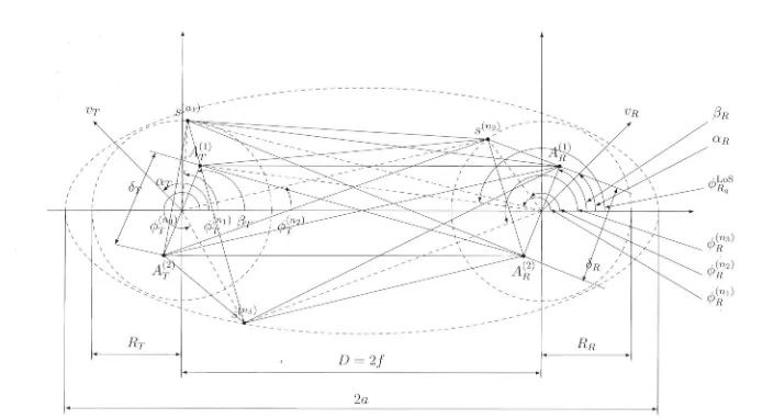
The Combination of a Two Ring and an Ellipse Model

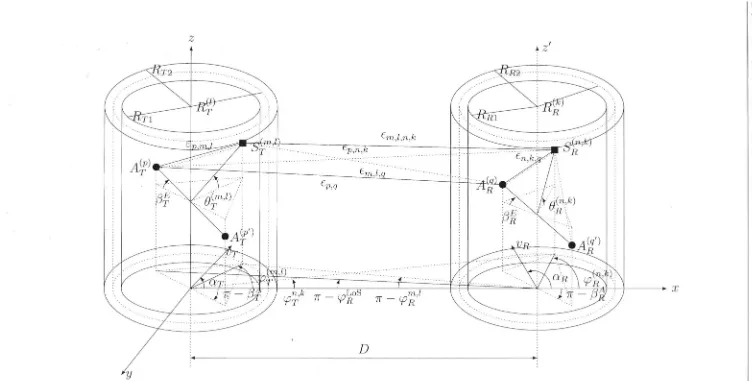
This model is a combination of a single- and a double-bounce two-ring model, a single-bounce ellipse model, and the LoS component [13]. The geometry of this model is shown in Fig. 2.7 where both nr and nR are equipped with omnidirectional

low elevation antennas. As an example, uniform linear antenna arrays with nr =

nR

=

2 are u ed here.

In Fig. 2. 7, 5(ni) represents the n₁th ( n₁

=

1, ... , Ni) effective scatterer lying

on a ring of radius Rr. Similar notation applies to 5(n2₎ _and₅_(n3₎_. _In_the_case_of

5(n3_),_N

3 effective scatterers lie on an ellipse with the Tx and Rx located at the

foci. vVhen

f

denotes the half length of the distance between the two focal points

of the ellipse, the distance between the Tx and Rx is given by D

=

2f.

1. In this model, it is normally assumed that Rr and RR and the difference

(54)

I I I I I I Vy / / / I I I I \ \ ' ' ' ' ' ' '

',,~~,~-

--Rr VR

RR

D =

2.f

2a

f3R

O'.R

<pLoS

Rq

¢~3)

¢~2)

¢~1)

Figure 2. 7: A generic channel model combining a two-ring model and an ellipse model with LoS components, single- and double-bounced rays for a MIMO M2M channel.

tv w ~ tv ~ Q P"' § ~ (D ... ~ 0 p_. (D ...

[image:54.882.106.811.92.473.2]

(55)

32 Review of l\Iobile to l\Iobile Channel Models, Measurements and Simulations than the antenna element spacings 5r and 5R, i.e., min{Rr, RR, a -

f}

>>

max{ 5r, 5R

}-The AoA of the wave traveling from an effective scatterer S(ni) ( i E { 1, 2, 3}) toward the Rx is denoted by <p~i). The AoD of the 'Nave that impinges on the

effective scatterer S(ni) is designated by

l;i)

.

Note that ¢~0s denotes the AoA of

q a LoS path.

The MIMO fading channel can be described by a matrix H(t)

=

[hpq(t)]nRxny of

size nR xnr. The received complex fading envelope between the pth (p

=

1, .. . , nr)

Tx and the qth (q

=

1, ... , nR) Rx at the carrier frequency fc is a superposition of the LoS, single-, and double-bounced components, and can be expressed as:

(2.64)

where

(2.65)

i=l

"[? f ( '(ni) ) 2 f ("'(ni) )]

X eJ ~1r Tmax t cos <Py -~IT + Ti Rmax t cos '+' R - 1 R ₍₂_.₆₆₎

and

(2.67)

The Combination of a Two Ring and a Multiple Confocal Ellipses Model

Mobile to mobile channel modelling for wireless communications