Large alphabet sequence modelling a comparative study

Large-Alphabet Sequence Modelling

A Comparative Study

Wen Shao

Supervisory Panel Chair: Marcus Hutter

May, 2014

Declaration

This thesis is an original work. None of the work has been previously submitted by me for the purpose of obtaining a degree or diploma in any university or other tertiary education institution. To the best of my knowledge, this thesis does not contain material previously published by another person, except where due reference is _{made in the text.}

w~

Sh~

-;;~

'

~v\

;)-/I

/0£(2--014-_

Acknowledgements

Foremost, I would like to express my sincere gratitude to my supervisor Prof. Marcus Hutter for the continuous support of my Masters study and research, for his patience, motivation, enthusiasm, and immense knowledge. His guidance helped me in all the time of research and writing of this thesis. I could not have imagined having a better supervisor and mentor for my Masters study.

I thank my fellow labmates in Reinforcement Learning Group at the Research School of Computer Science at the ANU: Tor Lattimore, Mayank Daswani, Hadi Afshar, for the stimulating discussions, for the sleepless nights we were working together before deadlines, and for all the fun we have had in the last two years.

Abstract

Most raw data is not binary, but over some often large and structw-ed alpha-bet. Sometimes it is convenient to deal with binarised data sequence, but typically exploiting the original structure of the data significantly improves performance in many practical applications. In this thesis, we study Martin-Liif random se-quences that are maximally incompressible and provide a topological view on the size of the set of random sequences. We also investigate the relationship between binary data compression techniques and modelling natural language text with the latter using raw unbinarised data sequence from a large alphabet. We perform an experimental comparative study for them, including an empirical comparison be-tween Kneser-Ney (KN) variants with regular Context Tree Weighting algorithm (CTW) and phase CTW, and with large-alphabet CTW with different estimators. We also apply the idea of Hutter's adaptive sparse Dirichlet-multinomial coding to the KN method and provide a hew-istic to make the discounting parameter adaptive. The KN with th.is adaptive discounting parameter outperforms the traditional KN method on the Large Calgary corpus:

Keywords

Contents

1 Introduction

2 Notation and Preliminaries

3 Small-Alphabet Sequence Compression Techniques 3.1 Kolmogorov Complexity and Martin-Lof Randomness

3.1.1 Plain Kolmogorov Complexity . . 3.1.2 Prefix Complexity . . . 3.1.3 Randomness and Halting Probability 3.1.4 A Topological View on Random Reals 3.2 Stationary Memoryless Source

3.2.1 Arithmetic Coding . . . . 3.2.2 Universal Coding . . . . . 3.2.3 Krichevsky-Trofimov Estimator 3.3 Stationary Source with Finite Memory

3.3.1 Binary Context Tree Weighing Algorithm 3.3.2 Model Class and Redundancy . . . .

4 Large-Alphabet Sequence Compression Techniques 4.1 Sparse Sequential Dirichlet Coding .

4.2 Sparse Adaptive Dirichlet-Multinomial Coding

5 Text Modelling Techniques 5.1 n-gram Models over Sparse Data 5.2 Smoothing Techniques . . . . . .

5.2.1 Additive Smoothing 5.2.2 Jelinek Mercer Smoothing 5.2.3 Absolute Discounting . . . 5.2.4 Kneser-Ney Smoothing . . 5.2.5 Modified Kneser-Ney Smoothing. 5.3 Pitman-Yor Process. . . . . .

5.3.1 Dirichlet Distribution and Dirichlet Process 5.3.2

5.3.3

Stick Breaking Representation and Chinese Restaurant Process Hierarchical Pitman-Yor Process . . . . . . .

11 13 18 19 20 22 23 24 27 27 30 34 34 35 36 38 38 39 41 41 41 42 43 43 44 45 46 46 47 49

6 Experiments and Discussion 51

6.1 Kneser-Ney and Binary CTW . . . 53

6.1.l CTW Implementation Notes . . 54

6.1.2 Kneser-Ney and Regular CTW 58

6.1.3 Kneser-Ney and Phase CTW 61

6.2 Large-alphabet CTW with Sparse Adaptive Dirichlet-multinomial Coding 62

6.3 Large-alphabet CTW on Artificial Data . 65

6.4 Applying SAD to Kneser-Ney . . 67

A Explicit Equations for Kneser-Ney

B Table of Notation

76

1

Introduction

Personal motivation. Compression is of great practical importance. It is widely used in data storage and data transmissions, especially with the advent of the Internet. Loosely speaking, the task of compression is to describe the data coming from a certain source as compactly as possible, which is achieved generally by devising a coding scheme according to a certain predetermined performance criteria, e.g., redundancy. There are two types of compression techniques: lossy and lossless data compression. The former is based on the assumption that some level of information loss can be tolerated and sometimes is necessary for storage purposes. For instance, a lossy compressor may remove non-audible components of a audio signal because humans can only hear a certain range of sound frequencies. In this thesis, we are, however, only interested in lossless compression, in which one could reconstruct the original data entirely and exactly from its encoded version using some computable decoding process.

Beyond its practical importance, compression is also theoretically and philosophi-cally interesting. Science is about learning from the past and predicting the future, at least to a large extent. For example, what is the weather going to be like tomorrow given the weather in the past several years. Many scientific problems can be reformulated as sequence prediction problems. Take the classification problem for example, with the training data being viewed as a sequence of (input, class label) pairs a classification problem can be re-expressed as a problem that given a training sequence and a new input one wants to predict the class label as accurately as possible. However, before be-ing able to predict the future well, as an intermediate step, one needs to understand the past, often by developing compact descriptions/representations of it, and we call such process learning. 1 _{In light of this, the first step in science is arguably about finding a} compact description of things we have observed. We then call such a representation a theory, a law or, in the field of machine learning, a model. As such, a major task for scientists is to represent/describe the observations more compactly and then use the discovered theories/laws/models to predict the data which cannot be observed directly or happens in the future. The problem of finding such a compact description of the past therefore lies at the heart of science and is a fundamental problem.

Although most real-life data is over some large and structured alphabet and may take different forms, for example text data consisting of a sequence of letters or words or a movie made up of images, one of the treatments is to convert them into binary sequences first regardless of its original high level structure. Data can easily be bina-rised, and in fact is binarised in all modern computers. As w~ will see in this thesis,

1_{VVe note, however1 that induction/learning and prediction can occur together. The learning process}

may not always explicitly happen prior to prediction. For example1 a binary sequence x1:n that is sampled independently from a Bernoulli distribution Bern( 0) with unknown 0 being the probability of X, = 1 for all i. The task is to predict the continuation Xn+l as accurately as possible. There are at least two perspectives on this problem. The first one involves an explicit learning process that learns/estimates the unknown 0 using the observations Xi:n, then, as a second step, to predict Xn+J using the estimated 0(xLn)-However, the prediction can also be done without having explicitly estimated 0. For example, if we have a prior belief on all possible 0's, denoted as 11"(0), then we can construct a distribution ~(x)=

f

0

1

K(0)P(xl0)d0, often called Bayes mixture. The conditional probability ~(Xn+1lx1,n) can be used directly for prediction. However, the induction/learning process in either case, explicit or implicit, is indispensable to prediction.

sometimes one can safely ignore the original data structure. e.g. for most parts in Algo-rithmic Information Theory (AIT). Also data compression is often studied for large but theoretically convenient universal classes of binary sequences and as a second step, if at all. adapted to larger alphabet. i\Iany asymptotic compression results are derived for binary alphabet and have strong theoretical guarantees only for small alphabet. How -ever, when it comes to practical data compression or modelling, exploiting the original structure of the data can substantially improve performance. Hence data compression and modelling for concrete tasks are usually done on the original or suitable represented data. as opposed to binary data.

This thesis investigates the relationship between these two paradigms and exper i-mentally compares the approaches used in binary data compression and large-alphabet data modelling. As a prototypical example for the latter, we take here document anal -ysis or more specifically statistical natural language processing.

2

Notation and Preliminaries

In this section, we introduce notation used in this thesis and some basic preliminaries. We use N,N0Z,IQ),IR to denote the sets of natural numbers ( {1,2, ... } ), natural numbers including zero ({0,1,2, ... }), integers, rational numbers, and real numbers respectively. S is used to denote a generic set. The size/cardinality of a set S is denoted by

I

Si.

S 1 US₂ and S₁ nS2 denote the union and intersection of two sets respectively. S 1 - S2

denotes the relative complement of S2 in S1 . In certain settings all sets under discussion are considered to be subsets of a given universal set !1. In such cases, !1-S is simply

called the complement of S, denoted by

sc

.

The power set of a set S is the set of all subsets of S, including S itself and the empty set, denoted by 25_{. If not explicitly} stated otherwise, lower-case letters i,j,k,n are used to denote natural numbers and

t

represents discrete time steps. Vve use(·,-) to denote some one-to-one mapping from N2

to N, that is, this function associates a unique natural number (x,y) EN with each pair (x,y)EN2_{. For example,(·,-) can be defined as y+(x+y+l)(x+y)/2. Iverson}

bracket is used in its common sense, that is

JI[Pl=

{

~

if _otherwise Pis true

Inequalities.

<,

>, <;,

?.

are standard inequalities. Let J, g be real valued functions. +

We write f(x) ?_g(x) if there exists a constant c such that f(x) ?_g(x)+c for all x.

+ + +

f(x)<;g(:i;) is defined similarly. f(x)";g(x) if f(x)?.g(x) and f(x)<;g(x). We write

J(x)?_g(x) if there exists a constant c>0 such that J(x) ?_cg(x) for all x. J(x) Sg(x)

is defined similarly. J(x)~g(x) if J(x)?_g(x) and J(x) Sg(x).

Finite strings. We are concerned with strings over a non-empty finite set X of letters or symbols. We use letters and symbols interchangeably to mean an element in X. We are primarily interested in binary set JIB= {0,1} as an example of small alphabet and some generic, but normally large finite alphabet X. In this thesis, we use 'string', 'word' and 'sequence' almost synonymously; however, we tend to use 'string' and 'word' to refer to finite strings and 'sequence' to refer to infinite ones. If not explicitly stated otherwise, lower-case letters x, y, z are used to denote finite strings (from some X'), E to denote the empty string and w=w1w2w3 ... infinite sequences (from some X00

). The length of a finite string x is denoted by C(x). The ith _{symbol of a string xis denoted}

by xi (0 < i

<:: C(x

)).

x

n

is the set of all strings over X of length n. The set of all finite string over Xis denoted X'. Substrings are denoted xici :=xixi+l···xj where i,j EN and i

<::

j. If i > j, then Xicj = E. A useful shorthand is x« := Xu-i- Strings may be concatenated. Let x,y EX' of length n and m respectively. Then,

xy:=X1Xz ... Xn-1XnY1Y2···Ym-1Ym

"·ithout am· out-of-set element to separate the words in the message. For example, modern English uses a white space to separate words because English vocabulary itself is not a prefix-code. For instance, a concatenated string 'farsidebag' can be segmented into 'far sidebag' or 'farside bag' or 'far side bag'. In many situations, a prefix-code is preferable. For finite binary srings, we can construct a prefix code for a subset S <;;;IIB' in the following way: given a string x ES, its ith _{order prefix-code word given by the} function E; · IE,' -) IE,' is defined recursively

{

FO

E;(x)= E;_₁(l(x))x

for i=0

otherwise (1)

There is a bijective mapping between IE,' and N, i.e., every element in IE,' can be paired with exactly one element in N. For example, we get a bijection if we map number iEN

to xEIIB' if i+l has a binary expansion of lx. The natural number 4 is mapped to the

binary string 01. We do not distinguish these two sets in this thesis. In Equation ( l), F denotes concatenation of x many l's, with x interpreted as a natural number. For example, E0(01)=1111 0, E 1(01)=110 01 and E2(01)=101 01. Analogously a string x

is called a (proper) suffix of y if there is a z(IE) such that zx=y. We use the function

# : X-) N to count the number of occurrence of a certain symbol in some understood corpus and relatedly#,: Xx

x

1_-1 _{-)]':J to count the number of occurrence of x, in xu-r,} that is, #,(x,lx11-1)=I:;;:;n[x;=x,]

Infinite sequences. The set of infinite sequences is denoted as X00 , which is the

infinite product of X with itself. A point (an element) in ;\:'00 is a one-way infinite

sequence, normally denoted by w = w1"'° = w1w2w3 .. with w; EX for all i. Vl/e are

particularly interested in IE,00 , which contains many interesting elements, for example the

element with w; = 1 if i is a prime number and wi =0 otherwise. Finite binary strings may

be concatenated with infinite sequences. For a finite binary string x = x1,n = x1x2 .. Xn and an infinite binary sequence w =w1,00 =w1w2 ... , their concatenation is

XW=X1Xz, .. XnW1W2 ..

The binary expansion of a real number r E [0,1] establishes a mapping between IIB00 and [0,1]. Given an infinite sequence w100 EIIB00 , a function f: IIB00 -) [0,1] maps it to the set of reals in the following way

~ W n 0.w:=f(w100)= 02n

n=l

We note, however, that this is not a bijective mapping. In fact, IIB00 is homomorphic to

the Cantor set, and hence is called a Cantor space.

(Un)Countable sets. Mathematically, a set is a collection of elements. A countable

set is in some sense a small set that has the same cardinality as some subset of the set of N. Formally,

Remark 2. If f is also subjective and therefore bijective, then S is called countably infinite.

Probability measures. A (probability) measure characterises the size of a set, more precisely, the size of a subset of some set fl. If fl is finite, it is a trivial task to describe the size of any of its subset, for example, just by simple counting (we also call it a counting measure); however, this method is not going to work when fl is an uncountable set, because otherwise any uncountable (or infinitely countable) subsets of a uncountable set would end up with having equal size, which is not very useful. The concept of measures helps to extend the idea of probability from finite (or countable) sample spaces to continuous ones.

Axiom 3 (Axioms of u-algebra). Given a non-empty set fl, 2n denotes the power set of fl. A<;;; 2n is a u-algebra if it satisfies the following.

1. flEA.

2. (A is closed under countable union) If A1,A2, . . is a countable sequence of elements in A, then the union

LJ~

An EA.

3.

(A is closed under complement) If

AEA,

its complement

Ac

EA.

We call an element in A a measurable set or an event in a probabilistic setting.

Remark 4. The axioms do not say that all subsets of fl, denoted by 2n, are measurable. In fact, there are many trivial u-algebras that obey the axioms, for example the set {fl,0} is a valid u-algebra of fl.

Axiom 5 (Axioms of probability measure). A probability measure defined on a u -algebra A of fl is a function P: A ➔ [O, 1] that satisfies

1. P(fl)

=

1

2. (Countable additivity) For any countable sequence

{An};:'=

1 of pairwise disjoint

events (for any

A;

,

A

1 E {

An};:'=

1 where i f j, A;nA1 = 0)

p

(QAn) = tP(An)

The value

P(A)

is called the probability measure of the event

A,

or simply the probability of A.

We note, however, these axioms can only be used to verify whether a given function is a valid probability measure and they tell little about how to construct a (non-trivial) probability measure over fl. In general this is not easy. One can instead define P

on some geometrically well shaped sets from which a measure on fl can be generated. One can formalise this idea and define probability measures on a continuous space X00

for some finite non-empty X. Consider a continuous space X00

, then a cylinder set is

Definition 6 (C:"1incler set). A cylinder set is a set r,cX00 _defined

by

r, := {xw:wEX00 }

"·ith .rEX'.

Geometrically speaking, a cylinder set can be identified with a half open interval in

[0.1). For instance, consider the cylinder sets in lIB00

, which are defined by fx={xw:wE JIB00_{} with .rElIB'. We can associate fx with a unique half open interval [0.x,0.x+2-£(xl}

), "·here O.x is the real number with binary expansion x. The length of the interval is 2-r(x)_ Note that xis a (proper) prefix of y iff fy<;; (c)fx.

Definition 7 (probability measure on X00 _{and probability dist}

ribution on X'). Let (] = {r x: x EX'} be the set of all cylinder sets in

x

=

.

Let A be the minimal er-algebra containing(]. A function µ: A--+ JR: defines a probability measure if

µ(r,)

µ(fx) 1

I > (rxul

yEX

A function P: X'--+ [0, l] is a probability distribution if L xEx· P(x) = 1

We write µ(x) to denote µ(f x). µ(x) is the µ-probability that a sequence starts with x. µ(y[x) :=

~'c;/

is the conditional probability of observing y EX given that x EX'

has already been observed. In particular, we use[, to denote the uniform measure i.e. L(x)=IXJ-f(x) for all xEX'.

Information theory. C.E. Shannon in his famous paper [Sha.!8] laid the foundation of

information theory. An important concept in information theory is the entropy, defined

as follows

Definition 8 (entropy). Given a finite/countable set n with a probability distribution P. Let P(x) be the probability of xE!:1. The entropy of Pis defined by

1 H(P) := L P(x)logP(x)

xE!l

The choice of logarithm base fixes the units used to measure entropy, but is otherwise unimportant. Common choices include base 2 that implies a measurement in bits and base 8 that implies a measurement in bytes.

Information theory is concerned with communicating a message between a sender and a receiver. Mathematically speaking, consider a non-empty finite/countable set

Theorem 9 (Shannon coding theorem). Let Lp and P as above.

H(

P

)

is the entropy of P, then

H(P)$.Lp$.H(P)+l

3

Small-Alphabet

Sequence Compression

Tech-niques

Kolmogorov Complexity and

Martin-Liif Randomness

Theoretical foundation

Small alphabet Large alphabet

Memoryless

I

I

KT Estimator

I :

~ -M- -~u,-met•i·c 1

~---+---Coding ~ - - : -.. ,,.~ I

I

I

SAD

Distribution is known

I

CTW_with KT

I

I

CTWwith SAD

I

Estimator

I

I I

Distribution With memory unknown

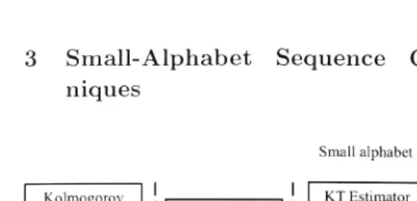
Figure J: The structure of the discussion on compression in this thesis.

The big picture and a general setting. The discussion on compression theories and techniques is unfolded according to the thread shown in Figure l. First, we present an overview of Algorithmic Information Theory (AIT) in this section. The purpose of surveying AIT is two-fold. First Kolmogorov complexity, a branch in AIT, can be co n-sidered as a theoretical foundation of compression. Secondly, Martin-Leif randomness,

another branch in AIT, is an interesting notion, opposite to compressibility. We will introduce Martin-Leif randomness and present our observations on the set of random reals in the unit interval.

'v\le then move to practical compression techniques. In this thesis, we are only

concerned with entropy coding methods, which, loosely speaking, is a type of lossless coding to compress data by representing frequently occmTing patterns with few bits and rarely occurring patterns with many bits. As such, we always assume that the to -be-compressed data is a sequence of source words from some finite alphabet X. For the convenience of the discussion later in this thesis and particularly for discussing universal coding, we present here a general setting. In many cases, e.g., the one in arithmetic coding, the setup can be simplified. Assume that there is a generating distribution P on X00 _and

P(x1,n) is the probability of the cylinder set of x1,n. In the compression

community, P is often tenned as a source or a model. 'Ne will use these two terms interchangeably. For a fixed

n,

P induces a probability distribution P"

(.x

1,,,

)

=

P(x1,,,) on the finite set X". Following P, the induced Pn is also called a source/model (on

X"). One wants to devise a coding scheme C,,: X" ➔ JIB' that generates a prefix-code for X", i.e. the co-domain of C,, needs to be a prefix-code. This kind of coding scheme

is often termed as Block to Variable (BV) code because the source words in X" are of the same length n and the source codes have variable lengths. In this thesis, we only

discuss BV codes. The number n is called the delay of the code in some compression literatures. <I>" is used to denote the set of all possible coding schemes on X".

[image:18.594.35.335.63.207.2]

used in compression is called expected redundancy and loosely speaking, it is the differ-ence between the expected code word length

Ep

j

£(1Cn

(x

1

,

n

)))

and the optimal expected

code length given by the entropy H(P n), where the expectation Epn is taken under P n· We start with introducing arithmetic coding as an example of a compression tech-nique when the distribution P is known. In practice, however, the generating distri-bution P is often unknown but can be assumed to be in a class/set of distributions. One wants to devise a coding scheme that is optimal in some weaker sense. We will introduce the notion of universal coding and investigate the notion of universality in terms of minimax redundancy. This domain can be further divided into four different sub-domains along two different dimensions. One dimension is on the characteristic of P, whether it is memoryless or with finite memory. We will introduce these two terms in this section and will survey both the KT estimator as an example of a coding scheme for memoryless generating distributions and the Context Tree Weighting ( CTW) algo-rithm with a KT estimator as an example for dealing with generating distributions with finite memory. The other dimension we consider is on the size of the alphabet X. The two methods mentioned above are particularly good for small alphabet, however, are not suitable for large alphabet. We will introduce Hutter's Sparse Adaptive Dirichlet (SAD) coding scheme as an example of a coding scheme designed for large alphabet in the memoryless case. We have also combined the SAD with the CTW algorithm, which will be used as an example for dealing with sources with finite memory over a large alphabet. SAD is introduced in Section 4 and the CTW with SAD is in Section 6.

3.1

Kolmogorov Complexity and Martin-Lof Randomness

A brief introduction. Algorithmic Complexity (AC) or Kolmogorov Complexity is a sub-field of AIT that lays the theoretical foundation of compression, which, loosely speaking, concerns the ultimate compressed version of an object and measures the (in)compressibility of an object. It was actually Solomonoff who first formed the basic ideas about algorithmic complexity and proved the invariance theorem in his long jour-nal paper [80164], but it is a tradition to talk about 'Kolmogorov complexity' instead of 'Solomonoff complexity'.

Imagine we want to describe a certain object using a binary string; intuitively the shorter the description the simpler the object. For example, the string x

=

01000 _seems simpler than string y=01011101010101101010101 even though the former is much longer than y. This is because we can easily describe x as 'one thousand zeros', whereas there is hardly any shorter description for y than literrally writing it. down. This is the main idea of Kolmogorov complexity, which measures the ultimate information content in an object. A big issue is that the length of a description depends on the choice of the language used to describe objects. It can be hard to describe a certain thing in one language, but very easy in another. For instance, before coffee was introduced to China there wasn't a word for it, and thus describing 'coffee' in Chinese was much harder than describing it in English. We therefore would like something fair among different languages, i.e. the complexity of a certain object should be invariant with respect to different languages in which we use to describe it.

is a probability distribution. whereas Kolmogorov complexity looks at the information

content of an individual object.

I--:olmogorov complexity is naturally connected with another philosophical notion

-randomness. Generally speaking, we would intuitively expect random things to be hard

to describe and, therefore hard to compress. There has been a long-standing debate

as to whether there exist true randomness in the universe or in nature. Some have

argued that everything is predetermined: and that seemingly random processes are

merely products of our ignorance. By contrast, others have suggested that the world is

objectively indeterministic. If we push the second viewpoint to the extreme and assume

that there is no pattern at all in nature, then scientists would not be able to compress

the observations and thus would not be able to learn (find models/theories/laws).

Con-sequently nothing would be predictable. Philosophically there are two camps as to this

issue: one is known as determinism and the other indeterminism.

If we turn our attention from nature to mathematics, we will see that back to the

time of Hilbert, mathematicians regard mathematics as absolute truth. Hilbert tried hard to formalise everything in mathematics into a small set of axioms and also proposed that mathematics is so precise that we can have some external machines to check the validity of our proofs. However, some work by Chaitin, e.g. in [GOO63, Cha86], showed a negative result that there exist infinitely many mathematical facts that cannot be effectively compressed into a finite set of axioms. The proof is based on the famous halting probability.

As well as providing philosophical insights, AIT has many applications. For exam-ple, Solomonoff's universal prior ( [Sol6.J., S0175] for induction and Hutter's universal artificial intelligence [Hut05]. One of the most interesting application is the universal similarity metric [LCL +03], which measures the similarity between string x and y as the length of the shortest program that computes

x

from

y

(i.e.

K

(xjy))

.

By proper normalisation and symmetrisation, this idea yields a universal similarity metric.

3.1.1 Plain Kolmogorov Complexity

The plain Kolmogorov complexity of an object is defined in terms of the information quantity that is required to losslessly describe it, i.e. one should be able to restore the

full object just from this description. Among all possible descriptions we choose the

shortest one. Formally, the plain Kolmogorov complexity is defined as following [L\"08].

Definition 10 ((plain) J{olmogorov complexity). Let

x,y,p

be finite binary strings. Any partial recursive function ¢:JIB*---+ JIB*, together with

p

and

y

,

such that ¢(

(y,p))

=

x

,

is a description of x given y. The (plain) complexity C¢, of x conditioned on y with respect to ¢ is defined by

C¢(xjy) =min{£(p): ¢(

(y

,

p))

=

x

}

,

p

where e(

p)

is the length of a program

p

,

and

C

¢(xj

y)

= oo if there are no such

p.

We

call p a program to compute x by <b, given y.

The requirement of 9 to be (partial) recursive is natural because we want to recon

that the complexity of x given y depends on the partial recursive function ¢ and for different ¢ the complexity of x varies. One would reasonably regard the complexity of a string as its intrinsic property that is independent of the partial recursive function. The following theorem [Gac07, LV0S] solves this problem to some degree.

Theorem 11. There is a universal partial recursive function ¢0 such that for any partial recursive function ¢,

C,t,0(x) <::C,t,(x)+c

+

or simply C,t,₀(x) <:'. Cq,(x), where c is a constant that is independent with x.

That is, the Kolmogorov complexity of any string x with respect to ¢0 is no longer than that with respect to any other partial recursive functions up to some constant c that is independent of x. Such a function ¢0 is normally termed as an additively optimal universal partial recursive function. As such, fixing such an additively optimal universal ¢0, the subscript of C is discarded and define the (plain) Kolmogorov complexity as C(xly)=C,t,0(xly). The unconditional complexity is defined as C(x)=C(xle) where e is

the empty string.

Complexity and incompressibility. \'le can consider p as a compressed version of x, and it is easy to see the length of x is a trivial upper bound for the length of p up to some constant. More formally, there is a constant c such that for all x we have

+

C(x) <:'. e(x) +c; we write C(x) <:'. €(x). This holds because we can simply construct a Turing that outputs whatever it is given. On the other hand, by a simple counting argument one can show that most strings cannot be (highly) compressed, that is, most strings are incompressible. The following theorem, which is due to Kolmogorov, reveals this fact [LV08].

Theorem 12 (incompressibility theorem). Let c be a positive integer. For each fixed y, every non-empty finite set AC JIB* of cardinality m(> 0) has at least m(l -2-c) + 1

elements x with C(xly)2logm-c.

If we set c= 1, we can see nearly half of the objects in a finite set whose complexity is almost the logarithm of the size of the set. This tells us that there is no effective way to (highly) compress the majority of objects in a set. This very fact suggests that we should think otherwise: instead trying to compress everything, we should only aim at compressing things that occur often and leave the rest. This fdea will be discussed in more detail in the subsequent sections.

C0~(.r)

=

1. As such. for any string x, there exists an additively optimal universal partial recursive function <f>x such that C,p, (x)

=

1. This issue may not show up when

studying asymptotic results using I<olmogorov complexity, but may yield dramatically different results when we study the complexity of a specific finite string. Scientists are uncomfortable with such context dependence. Discussions about this issue have been extensive, see for example [Stc10I]. It is clear that <Px would not be natural as it is engineered towards a specific x, however, how to rigorously formalise the notion of natural is a difficult problem. Some researchers [RHJ I] argue that we should always

use some predetermined and universally agreed-upon reference machines to start with before seeing the string we are studying. This argument does not solve the problem entirely as one can always claim that it is possible to accidentally choose a reference machine that yields low complexity for highly complex strings. [L\.08] claim that they found a mathematically clean solution to this problem, however, this solution is not widely accepted due to some flaws in their argument. As a result, this problem still remains an open question in this field [Hut09].

Another Achilles heel of AC is that C is necessarily incomputable, moreover, no partial recursive function

¢,(x)

defined on an infinite set of points can coincide with

C(x)

over the whole of its domain of definition. Due to its in-computability, it is hard to put AC to practical use. One can, however, approximate

C(x)

from above, i.e. there is a total recursive function 'lj;(x,t), monotonically non-increasing in t, such that

limt➔00ip(x,t)

=

C(x).

3.1.2 Prefix Complexity

Problems with plain complexity. Although the idea of plain complexity is ground-breaking and the results regarding it are very fruitful, it suffers from some problems that make it less mathematically beautiful. The most obvious one, as we have already mentioned in the previous subsection, is that plain complexity is not subadditive. The reason for that is that the description itself is not self-delimiting; once two strings are joined together there is no way to tell them apart without additional information. But we would like to have

C(x,

y)

'.,'. C(x

)

+C(y),

which coincides with our intuition. Unfortunately the plain complexity doesn't enjoy this property. These inconveniences call for another version of complexity, which has better mathematical properties.

Prefix functions and prefix complexity. The idea of prefix complexity was int ro-duced in [Lev7-l, G,\e7-l, Cha75b]. In order to overcome the aforementioned problems, partial recursive prefix functions are defined as follows:

Definition 13 (partial recursive prefix function). A partial recursive function ¢,: llll' -t

llll' is a partial recursive prefix function if and only if its domain is a prefix-code.

Analogous to plain complexity, a theorem in [L\108] states that there exists an additively optimal universal partial recursive prefix function

¢,

0 such that for every partial recursive prefix function

¢,

there is a constant

_c1

such that

C1

0

(xly)

'.,'.

C1(xly

)+c¢

3.1.3 Randomness and Halting Probability

There is a natural connection between randomness and Kolmogorov complexity; exte

n-sive research has been done in this area, for example, [Lev74, Cha75b, Cl\97, Sch73). Martin Lof randomness, first introduced in [l\IL66), is usually defined from a measure -theoretic perspective.

Definition 14 (Martin-Lof random). Let

{A;}

f,;

1 be any effectively enumerable infinite sequence of recursively enumerable(r.e.) sets of intervals2_{. Then w is Martin-Lo£ random} iff for any such sequence {

A;}

f,;

1

V{A;}~l: Vi, .C(Ai)~ri, 3j: w(/.Aj

where .C is the uniform measure. Equivalent definitions are given by Solovay and Chaitin [Cha75b). Their equivalence is proved in [GC89).

The basic idea of this definition is that if a sequence is random, then it cannot have any constructive distinguishing features; in other words, it cannot be expressed easily.

For instance, a sequence w=(01)00 _{is (intuitively) not random, we}

can easily construct a descending sequence of intervals such that every interval contains this sequence. Also

this sequence is very easy to describe, namely 'repeating Ols'.

A celebrated result is given by Chaitin who showed that for the prefix complexity

K(x), random sequences in Martin-Lof sense with respect to the uniform measure are

those sequences for which the complexity of each initial segment is at least its length

(up to a constant).

Theorem 15. An infinite binary sequence w is Martin-Lo! random with respect to the

uniform measure if and only if there is a constant c such that for all n, K(w1,n) ?.n- c.

This result explicitly tells us that the random sequences are the complex ones, and there is no effective way to compress them. Indeed, if there exist a c such that

K(w1,n)

<

c for all n, then there must be a program p of finite length that generates w and we will not call it a random sequence because the patterns in it can be described within f.(p) bits.

Numerous results have been discovered based on this theorem, and one of the most

interesting ones is that the halting probability is random in Martin-Lof sense. The

halting probability is the real number S1= I:u(p)<oo2-L(p), and the sum is taken over all

inputs p for which the reference machine U halts. S1 is also known as the number of wisdom. Unfortunately, although this number can be approximated from below, it is random with respect to the uniform measure and thus is maximally unknowable.

Mathematical facts can be random. Hilbert proposed that we could construct some external machines to automatically prove theorems. There are at least two attacks on

the thesis of Hilbert. The first one is the well-known 'halting problem'. We will be concerned with the second one, which is given by Chaitin [Cha71, Cha75a, Cha82,

Cha86). He constructed a sequence of mathematical facts, which are rigorously well defined and which are random, i.e. these facts can't be compressed into a smaller set

of axioms and they are irreducible mathematical information. To see this, we need the definition of Diophantine.

2_{For a self-contained introduction to Martin-Lof random, plea}

Definition 16. (Diophantine) A set AC

zn

is Diophantine. if there exists a polynomial P(_a1 .a_{2 ....} an.Xi .x₂ . ... :r,,,) with integer coefficients such that

A= { (a1

---,Cln)

E Z"l::l(x1,

-

--

Xm)

E zm ,s.t.P(a1 , ....

a,,

,

x

,

,

....

xn,)

=0}

There is a well-known theorem that says a set of tuples of positive integers is Dio-phantine if and only if it is recursively enumerable (r.e.). Now consider a computable increasing sequence of rational numbers { rk });0=1 with limk--+oork

=

11. Construct set A which contains tuple (n,k) such that nth _{bit of rk is 1. A is r.e. and thus Diophantine.} Hence there exists a polynomial P'(k,n,x1 ,x2,---,xm) which equals O if and only if n"' bit of r;- is 1. Consequently, the set D~

=

{xl::ly1,Y2,---,Ym[P'(x,n,y1,y2,---,Ym)

=

OJ} is infinite iff the nth _{bit of the base-two expansion of [1 is a 1. Now one can easily see} the equivalence between whether

D;

,

is infinite and whether the nth _{number of [1 is 1.}

Note that the first is either true or false; however, these mathematical facts can't be compressed into a smaller set of axioms. They are irreducible mathematics information. This can be considered as a quantification of Godel's incompleteness theorem.

3.1.4 A Topological View on Random Reals

We are interested in characterising how large the set of random sequences is. We study this from three different perspectives: set theoretic, measure theoretic and topological perspective. For simplicity, let Rand denote the set of random infinite binary sequences and let NonRand=E00_{- Rand. The following definitions and remarks are helpful for} our discussion.

Definitions. Intuitively, countable sets are smaller than uncountable ones. The set of rational numbers and the set of computable sequences are countable. The set of real numbers and the set of irrational numbers are both uncountable.

Definition 17 (dense). A set S <;; [0,1] is dense in the interval I if S has a nonempty intersection with every subinterval of I; it is called dense if it is dense in [0,1].

Density is a topological notion which describes how a set S is distributed. The set of rational numbers in [0,1] is (everywhere) dense (in [0,1]), but no finite set of real numbers in [0,1] is (everywhere) dense (in [0,1]).

Definition 18 (nowhere dense). A set S is nowhere dense if it is not dense in any interval, that is, if every interval has a subinterval contained in the complement of S.

Intuitively a nowhere dense set is 'full of holes'. An alternative but equivalent definition is that a set S is nowhere dense if and only if its complement

sc

contains a dense open set.

Definition 19 (first and second category). A set S is said to be of the first category or meagre if it can be represented as a countable union of nowhere dense sets. A subset of [O, 1] that cannot be so represented is said to be of second category or non-meagre.

is that sets of second category are denser than sets of first category. It follows that no

interval in [0,1] is of first category, the set of rational numbers is first category and

Cantor set is of first category (even though it is uncountable).

Lebesgue measure is another way to measure the 'size' of a set from a sampling perspective: The larger the Lebesgue measure of a subset is, the larger the set is.

We also need to introduce two classical lemmas for our discussion, the proofs of which can be found in any mathematics analysis textbooks (e.g. [Zor04] and [RFlO]).

Lemma 20. The Cantor set, defined as

oo 3rn-1 _1

C=[

O

,

l

]\

LJ

LJ

(3k

+

l 3k+2

m=l k=O 3m ' 3m )

is uncountable and nowhere dense in [0,1].

Lemma 21. Any subset of a set of the first category is of the first category.

Interesting facts about Rand. We study this from three different perspectives: set theoretic, measure theoretic and topological perspective. The known facts are s

um-marised in Table 1.

Item Category Measure Cardinality Density Example

1 first 1 countable dense not exist 2 first 1 countable nowhere dense not exist 3 first 1 uncountable dense Rand 4 first 1 uncountable nowhere dense not exist 5 first 0 countable dense IQ

6 first 0 countable nowhere dense single point

7 first 0 uncountable dense exist, constructive[WH93]

8 first 0 uncountable nowhere dense Cantor set 9 second 1 countable dense not exist 10 second 1 countable nowhere dense not exist 11 second 1 uncountable dense [0,1]- l(ll

12 second 1 uncountable nowhere dense not exist 13 second 0 countable dense not exist 14 second 0 countable nowhere dense. not exist

15 second 0 uncountable dense NonRand

16 second 0 uncountable nowhere dense not exist

Table 1: Sixteen combinations of set size characteristic from set theoretic, measure theoretic and topological perspective. Examples are given in the last column.

We have the following observations [Ca102].

2. From a measure-theoretic point of view, Rand has measure 1 in the sense of

Lebesgue. whereas N onRand has measure 0. This result shows that if sample

from IB\00 _{according to uniform distribut}

ion, one will get a random sequence with probability l.

3. From a topological point of view, with the ordinary topology on [0,1] both sets are

everywhere dense in [0,1], however, Rand is of first, category, whereas NonRand

is of second category. This result shows topologically the set of non-random

sequences is much denser than the set of random ones.

Cardinality, (Lebesgue) measure and density are ways to measure the size of a set but from different perspectives. Intuitively speaking (though not true strictly), uncountable sets are larger than countable sets; the larger the measure of a set is, the larger the set is; sets of second category are larger than those of first category. The last observation is very counter intuitive especially when compared with the second observation. Even though the set of non-random sequences are much denser than random sequences in [0,1], if one samples randomly then with probability 1 one will get a random one. The

third observation doesn't say that the set of non-random sequences is necessarily larger

than the set of random ones; it only says the former one is denser than the second one

in some sense. One example to best illustrate this involves the Cantor set and the set of rational numbers The Cantor set is uncountable and thus larger, in a certain sense, than the set of rational numbers which is only countable, but nevertheless the Cantor set is nowhere dense (defined later) and rational numbers are (everywhere) dense in

real.

Remark 22. A few remarks on Table 1:

l. Items 1,2,9,10,12,13,14,16 do not exist because: countable sets must have measure zero; nowhere dense sets must be first category; and countable sets must be first category.

2. Item 4 does not exist. More generally, any set that has measure 1 cannot be nowhere dense. However, there exists a nowhere dense set in [0,1] that has positive measure, e.g., the fat Cantor set.

Proposition 23. The set of nonrandom sequences with respect to the Lebesgue measure is of second category, whereas the set of random ones is of first category (Cal/l!l}.

We provide a different proof from the one in [Cal02].

Proof Fix an effective enumeration of all rational numbers in [0,1], IQ= {q1,q2 , ... }. Let

ln=U;1(qj-2-n-j-l,qj+2-n-j-l) and Ai=n~=]In-Then

{A

;}

is an infinite sequence

of r.e. sets of intervals. Now we put

A

=

A

00 and

B

=

[0,1]\A. We now want to show (1) every element in A is nonrandom; (2) B is of first category and thus A is of second category and (3) The set of random sequences is a subset of B and thus is of first category. For each

A

i,

we have

.C

(

A

i)

s..c(I

i)

s.

L.C((qJ

-

r

i-J-

1,qJ+r

i-

J-1))

=

L

ri

-

J

=

ri

For any elements w in A, we have w E Ai for all i. Hence (1) is true. Next we show B is of first category, observe B = LJ~

=l

I~ and I~ must be nowhere dense because it's

complement In is a dense open set, so B is a countable union of nowhere dense set and

thus of first category. The fact that AUE= [0,1] and AnB

= 0

implies A has to be

of second category, because [0,1] would be of first category otherwise. (3) is obvious because of the fact that any subset of a set of first category is still of first category.

This completes our proof. □

3.2

Stationary Memoryless Source

Following the setup at the beginning of this section, consider a non-empty alphabet

X with a source P and the induced distributions Pn on xn, if Pn(XLn)

=

fl7=1

P1(xi)

for all n, then the source P is called a stationary memoryless source and is identified

by the distribution P1 on X. The term 'memoryless' indicates that the conditional

probability of the nth _{symbol given the previous symbols P(xnlx<n) is equal to P1(xn)}

and thus independent of what has been observed in the past. In this subsection, we

only consider stationary memoryless source and in this subsection only, we drop the

subscript '1' in P1 and call it the source of the data. For example, we write 'a data sequence XLn E lllln generated from a Bernoulli distribution' to mean x1,n is sampled

from a stationary memoryless source that is identified with a Bernoulli distribution and

xi~Bern(0) for all iE{l,2, ... ,n}.

We first discuss the simplest case where the source P is known before turning to a

more realistic situation where we don't know the source in advance, but can be assumed

to be in some general class of sources.

3.2.1 Arithmetic Coding

According to Amir Said [Say03], arithmetic coding is a coding technique that is able to

work most efficiently in the largest number of circumstances and purposes and stands

out in terms of elegance, effectiveness and versatility. He also lists some of the most

desirable features of arithmetic coding.

The basic idea of arithmetic coding is that we fit any sequence into a subinterval of

the interval [0,1). The Elias algorithm provided the foundation of all arithmetic codes,

an early description of which can be found in [Jel68]. The principle can be traced back

to Shannon [Sha48].

Arithmetic coding process. Formally, given an input string X1,n, the arithmetic coding process yields a sequence of nested intervals

{[a

i,/Ji)}i=l

where the sequence

comes from a stationary memoryless data source with non-empty finite alphabet X.

Without loss of generality, it is assumed that X

=

{0,1,2, ... ,M -1}. The probability

distribution p(m)

=

P(xi

=

m) with m EX and i

=

1,2, ... ,n is assumed to be known in

advance. We define c(m) to be the cumulative distribution, i.e. c(m)

=

L','J'=~

1

p(j)

with mE{0,1,2, ... ,M}. Note that c(0)=0 and c(M)=l. ak and /Jk are real numbers with 0 '.::'. °'k-l '.::'. °'k '.::'. /Jk '.::'. /Jk-l '.::'. 1. To describe arithmetic coding, it is useful to introduce a new no_tation

In other ,rnrds. b is the starting point of an interval whereas l is the length of the interval. The inten·als used in arithmetic coding can be described by the set of recursive equations

Ibo.lo) lb;,l;)

I0,l)

lb;-1 +c(x;)l;-1 ,p(x;)l;_1 ). i

= 1,2,

... ,n

(2) (3)

This process. ,,·hich ,ms first described in [.J<'llii::i]. keeps the properties 0<::;b; <::;bi+, and

0 < /;+1 <I;<::; 1 and in doing so, we get a sequence of nested intervals. The final step of the coding process is to choose a code value for the sequence. Since given this coding scheme. each real number in the resulting interval

[

a:n

,.B

n)

represents a code (under the known source P) for a string that begins with X1cn, we are free to choose any real

number from [0,1) as the code of X1cn, provided that we (1) write the number of data symbols (i.e. n) in the compressed file, or (2) add a special symbol signalling the end of message. Naturally we want to choose a real number such that its representation

is the shortest with respect to the alphabet, over which the codeword is to be stored or transmitted. For example, if the codeword is to be stored in a physical computer or transmitted over the Internet, one wants to find a real number within the resulting

interval whose binary representation is the shortest ( trimming off the infinitely many ending zeros).

Arithmetic decoding process. Let r E [0,1) be the codeword for X1cn• Note that the

probability distribution and the length of the original word (i.e. n) is known to the

decoder. The decoding process recovers the original word in the same procedure that they were coded and can be expressed using a set of recursive equations

r1

X;

Ti+l r

m, s.t. c(m)<::;r;<c(m+l) i=l,2, . . ,n r -c(x)

-•-(_ )_, i=l,2, .. ,n- 1 p X;

Generalising the arithmetic coding to non-i.i.d. models. Arithmetic coding can accommodate non-i.i.d models in a very natural way. We have assumed an i.i.d. model

in the introduction to arithmetic coding, we now generalise it to non-i.i.d. models, e.g., sources with memory.

The memoryless model is a very simple model and it does not accurately reflect most real world sources, such as language, image, video, which are highly structured and have

interesting dependencies between the different symbols in the sequence. Unfortunately the simple i.i.d. model does not account for that. In order to make arithmetic work for

real world models, there is a need to the extend arithmetic coding to non-i.i.d models.

Formally, we have assumed that an input string Xin comes from a memoryless

data source with non-empty finite alphabet X

=

{0,1,2, ... ,.M -1 }. The distribution p(m) =P(x; =m) is known. The joint probability thus can be written as

n

P(x1n)= Ilv(x;)

Now consider an arbitrary known source model given by Q(x1,n), which always can be

factorised as (under weak regularity conditions)

Q(x1

n)

=

IJ

qi(xilx<i)

i=l

where

) Q(xli)

qi(xilx<i = Q(x<i)

is the conditional probability of Xi given all the previous symbols. Granted that these conditional probabilities can be easily computed, there is trivial modification to the arithmetic coding for memoryless models: We define the cumulative distribu

-tions ci(m) = ~7=-;/q(jlx<i) with m E {0,1,2, ... ,M} and modify the recursive process defined in Equation (3) to the following

lbo,lo) = I0,1)

lbi,li) =bi-I +ci(xi)li-1,qi(xilx<i)li-1), i = 1,2, ... ,n

where li remains to be the length of the interval. The rest of the process remains the same and the decoding process is modified accordingly.

Performance measure -Expected redundancy. A performance measure is needed to discuss the performance of arithmetic coding and any other coding methods. Many performance measures can serve this purpose from different perspectives, for example,

• Total or average code word length of a coding scheme. Formally, for a coding scheme IC and a data sequence X1cn, the total (average) code word length is given by £(1C(x1,n)) (£(1C(x1,n))/n). It is clear that this measure is not suitable for comparing coding schemes for compressing data sequences generated from

different sources, simply because the compressibility of the data sequences varies

with the sources. However, this is particular useful when comparing compression techniques on some benchmark corpora and thus widely used in practice. In my experiments, this measure is used for comparing different compression methods. • Expected total or average code word of a coding scheme. To avoid a

coding scheme from being engineered towards a particular string x1

,n,

expected

total or average code word of a coding scheme can be used, where the expectation is taken with respect to Pn over all X1cn•

• (Expected) Redundancy. This measure is commonly used in theoretical analy-sis and many results in the compression field are expressed in terms of redundancy. If a data sequence x1,n is sampled from some distribution P n, then the

theoret-ical ideal is to code it in -logP n(X1cn) bits and a lower bound on the expected

code word length is the entropy of the source H (P n). Any bits needed beyond -logP n(Xin) are considered to be redundant and the overhead is called redun-dancy for a particular data sequence x1n, that is, given a coding scheme IC, the individual redundancy is,

,d1ich takes both positive and negative values. Another reasonable measure is the expected average redundancy. that is,

R(Cn.Pn)

=

Ep,. (C(IC(x1n)))-H(Pn)

n (4)

Shannon coding theorem asserts that this quantity is larger than zero, and one aims to devise a coding scheme that minimises this quantity. In particular, if

lim R(Cn,Pn)=O

n---+oo (5)

then a sequence of coding schemes {Cn}~=l is called asymptotically optimal. One should note, however, that this optimality notation is rather weak, which will be discussed later in this thesis.

• Other measures. !VIany other measures are also used, for example, regret and perplexity. However, we don't use them in this thesis.

Optimality of arithmetic coding and its limitation. Arithmetic coding has been

shown to achieve optimal compression performance when applied to a stationary mem-oryless source [SaiO.J.], that is, let C0 represent arithmetic coding, P be a stationary memoryless source over a non-empty finite alphabet X, then

R(Ca,Pn) Ep,.(e(C.(x1n)))-H(P,,)

=

Ep,,(C(Ch1n))) H(P)

n n

tends to zero when n ➔ oo. In fact, the coding redundancy for any x1,,, is at most 2

bits. Despite of its optimality, we need to know a lot of information in advance, namely, the exact probability distribution that generates the sequence. In a real life problem, it is often too much to ask for. v\That if we don't know the probability distribution in

advance? In the next subsection, we deal with the case where we don't know the exact distribution but instead we assume a generic class of distributions, which so large that the true one is (hopefully) in this class.

3.2.2 Universal Coding

Motivation and setup. Arithmetic coding is effective and optimal if we know the

underlying distribution µ(Xi,n) in advance and code the sequence accordint to it. Uni-versal coding, on the other hand, deals with the situation where we know little about

the underlying distribution and hope we can do nearly (by some reasonable measure) as well as if we knew it. An apt example is given in [Grii07]: consider compressing a sequence x1,

n

,

which is generated by a Bernoulli model with unknown parameter 0. Suppose we believe that this sequence is sampled from

Ber

n(0')

and devise a coding

scheme Co, to code this sequence accordingly, that is, let n0 and n1 be the number of Os and ls in Xi,n, hence

n

0

+

n,

=n

,

then C0, will generate a code word of length -n1log0'- nolog(l-0') for Xin• If can be shown that the expected redundancy of

C0'

for a sequence of length n is

where KL(0ll0')=01ogf,+(l-0)1og;_:_-%, is the Kullback-Leibler (KL) divergence, which,

though not a proper metric, measures the distance between 0 and 0' in the sense that

KL(0110') 2:0 and only equal to O when 0=0'. For 0'f0, the redundancy will not tend

to zero, 311d thus 1[0, is not optimal. The question is then whether there exists a coding

scheme that regardless of the true distribution behaves nearly as well as arithmetic coding when the true distribution is known.

To formalise this question, suppose a data sequence x1,n is generated by a source

P, which is unknown but can be assumed to be in a set of sources

M.

The aim is to devise a coding scheme that is asymptotically optimal regardless of what the underlying distribution is in

M.

Indifference rule. Laplace, several hundred years ago, pondered the same question, but from a prediction perspective. He asked the following question, 'What is the prob-ability that the sun will rise tomorrow? (given it has always risen in the past)'. We can formally phrase this .question as follows: Given a sequence of x1,n that is generated i.i.d from a Bern(0) with unknown 0, what should be P(xn+i = llx1,n)7 Now that we have a class of models, namely the family of Bernoulli distributions, each member in this family is uniquely indexed by a 0E8=[O,l]. Following a Bayesian approach, we express our prior believe on 0 with the density function 11(0). To combine the infor-mation regarding our prior and our observed data, we use Bayes rule. We define the posterior distribution 11(0lx1,n) as

P(x1nl0)11(0)

11(0lx1 n) = feP(x1n10')11(0')d0'

(6)

This posterior distribution contains both sources of information that we have about

the parameter, namely, our prior beliefs and the observed data. This posterior distri-bution readily provides changes to our prior belief brought about by the data. The predictive distribution is then given by

P(xn+l = llx1n) =

l

P(xn+l = ll0)11(0lx1n)d0

(7)

If we are indifferent among all possible models (0), that is, to take a uniform prior distribution over 8 such that 11(0) = 1 for all 0 E 8, we end up with Laplace rule, that

is P(xn+l = llx1n) =

#;~t

1, where #(1) denotes the number of l's in Xin•

A-Priori distribution. We can easily show that this scheme is equivalent to predicting with the following Bayes mixture

P(x)

=

fe

11(0)P(xl0)d0 (8)

This can be interpreted as a mixture of all models (P(xl0)) weighted according to our prior belief over all possible 0E 8, expressed by 11(0). Assuming the true source is given

by Bern(0), the expected redundancy of a coding scheme i[p based on the mixture

P(x) in Equation (8) is

1 ~ P(xl0)

R(1Cp,Bern(0)) =;;;, L.., P(xl0)log r

811(0)P(xl0)d0