Machine Learning Molecular Dynamics Simulations for Enhanced Student Learning

Machine Learning Molecular Dynamics

Simulations for Enhanced Student Learning

Fanbo Sun, JCS Kadupitiya, Geoffrey Fox, Vikram Jadhao

Indiana University Bloomington, Indiana 47408

{fanbsun,kadu,gcf,vjadhao}@iu.edu

Abstract—Molecular dynamics (MD) simulations accel-erated by the use of high-performance computing (HPC) have enabled the understanding of microscopic mechanisms underlying the material and biological phenomena such as protein folding, ion transport across cell membranes, and nanoparticle self-assembly. In the context of using MD simulations in education, rapid simulation-driven responses to students in classroom settings are desirable in elucidating concepts and demonstrating the application potential of HPC. We explore the idea of integrating machine learning (ML) with HPC-accelerated MD simulations to enhance their usability for education applications. The idea is illus-trated using parallelized MD simulations deployed as a web application on nanoHUB and designed to extract the distri-bution of ions in nanoconfinement. We find that an artificial neural network-based regression model successfully learns nearly all the interesting features associated with the output ionic density profiles and rapidly generates predictions that are in excellent agreement with the results from explicit MD simulations. The inference time associated with the ML surrogate is over a factor of 10,000 smaller than the corresponding parallel MD simulation time. The dynamic, real-time and anytime engagement with the ML-integrated simulation framework can enable enhanced student learn-ing of concepts associated with basic and advanced topics in computational science and engineering.

Index Terms—Machine Learning, Molecular Dynamics Simulations, Parallel Computing, Scientific Computing

I. INTRODUCTION

Particle or molecular dynamics simulations are pow-erful tools for investigating the behavior of materials at the molecular and nanoscale. These simulations have enabled the understanding of microscopic mechanisms underlying the material and biological phenomena such as protein folding, ion transport across cell membrane, flow of polymeric liquids, and self-assembly of nanos-tructures. The molecular dynamics (MD) method solves the Newton’s equation of motion for a system of many particles and evolves the positions, velocities, and forces associated with these particles at each time step. While MD simulations are generalizable to study a broad range of molecular and nanoscale phenomena, they incur high computational costs because the computational

complex-ity per time step is proportional to the square of the total number of particles (system size).

The high computational costs associated with MD simulations are mitigated by employing high-performance computing (HPC) resources and utilizing parallel computing techniques such as OpenMP and MPI. An example of an MD simulation of confined ions [1], [2] illustrates the power of HPC-enabled simulations. For this system, ≈1 nanosecond of dynamics of≈500

ions on one processor takes ≈ 12 hours of runtime, which is prohibitively large to extract converged results for ion distributions within reasonable time frame. Using MPI or hybrid OpenMP/MPI techniques dramatically enhances the simulation performance: for systems with thousands of ions, speedup of over 400 can be achieved, enabling rapid generation of the needed data for evalu-ating converged ionic distributions.

computational science and applied HPC subjects. As an example, consider an MD simulation frame-work, Ions in Nanoconfinement, that we deployed as a web application on nanoHUB to execute the afore-mentioned simulations of ionic systems [3]. This tool has been employed every semester since Spring 2018 in illustrating concepts in a graduate course (Simulat-ing Nanoscale Systems) and an undergraduate course (Introduction to Modeling and Simulation) at Indiana University (IU). A video demonstration of the lecture on the use of the simulation tool and related compu-tational nanoscience concepts is available online [4]. In classroom usage, we observed that the fastest simulations took about 10 minutes to provide the converged ionic densities while the slowest ones (generally associated with larger system sizes) took over 3 hours. Primary factors contributing to this scenario were the time delays resulting from the combination of waiting time in a queue on a computing cluster and the actual runtime for the simulation. Not having rapid access to expected trends in the variation of ionic densities with input parameters made the process of explaining associated concepts (e.g., self-assembly, steric effects) unwieldy and time-consuming, and slowed down the training of students interested in pursuing a class project or per-forming introductory research on the subject.

Generally, the approach to provide instant simulation output is to store the previous simulation results in a cache (simulation caching). nanoHUB provides this as a feature in computational tools created using their GUI, Rappture. Cached simulations provide a static environ-ment with pre-selected parameters defining simulations that can be “looked up”. This simulation environment offers limited exploration space, interactivity, and re-sponsiveness to the student. To encourage and empower students to directly experiment and explore the nanoscale system and associated phenomena, a new approach is needed that delivers an interactive, dynamic, and respon-sive simulation environment open for wide exploration. Motivated in part by these challenges in employing state-of-the-art MD simulations in education, in a re-cent paper [5], we introduced the idea of integrating machine learning (ML) methods with MD simulations to enhance their usability for research and education. We demonstrated that an artificial neural network (ANN) based regression model, trained on data generated via HPC-accelerated MD simulations, successfully learns a small number of pre-identified features associated with the simulation output. The ML surrogate instantaneously generated predictions in excellent agreement with results obtained from explicit MD simulations.

In this paper, we extend the idea of integrating ML methods with MD simulations to the more challenging problem of capturing nearly all the interesting features

of the desired simulation output. We utilize the MD simulations of ions in nanoconfinement employed in our earlier work [2], [5] to illustrate the results. While the earlier paper showed a relatively small number (3) of ML-generated predictions for the ionic distribution (the contact, mid-point, and peak ionic densities), we now demonstrate that the ANN model trained on the same dataset yields accurate predictions for ≈ 150 output parameters, enabling the estimation of almost all the interesting features of the ionic density profile for a wide range of system parameters. The inference time associated with the ML surrogate is over a factor of

10,000 smaller than the corresponding MD simulation time. We anticipate that such an integration of ML with simulations to enhance their usability holds enormous potential for the use of simulation tools in education. The resulting overall improvement in the interactivity with the simulation framework in terms of dynamic, real-time engagement and anytime access can enable en-hanced student learning of concepts associated with more complex systems and state-of-the-art research topics.

II. BACKGROUND ANDRELATEDWORK

MD simulations serve as important tools for under-standing diverse self-assembly phenomena in nanoscale materials [6]–[8], predicting material behavior in prac-tical applications [9], and isolating interesting regions of parameter space for experimental exploration [10]. Recent years have seen a tremendous rise in the use of ML in enhancing simulations to predict parameters, generate configurations, and classify materials properties [11]–[17]. Despite the surge in computational materials research, the use of ML for associated education appli-cations has been relatively unexplored.

The authors are members of a relatively new engineer-ing department launched in 2016, Intelligent Systems Engineering (ISE), at IU. The ISE curriculum at both un-dergraduate and graduate levels builds on a strong HPC, information technology, and modeling and simulation core informed by application areas such as nanoengineer-ing and bioengineernanoengineer-ing. The last author teaches two core courses in the curriculum (Introduction to Modeling &

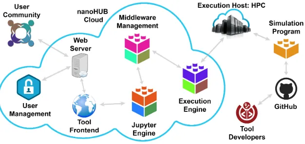
Fig. 1. Ecosystem of a computational tool deployed on nanoHUB.

The HPC-accelerated MD simulations are key parts of these courses. To facilitate their use by students in classrooms and for solving homework problems, the simulations are deployed as computational tools on nanoHUB [19]. nanoHUB provides online access for executing simulation codes to students and educators interested in nanoscale science and engineering. The authors and the extended research group members have launched 4 nanoHUB tools [3], [20], [21] exploring diverse self-assembly phenomena in nanomaterials. One of these tools, “Ions in nanoconfinement” [3], has been extensively employed by IU students to learn nanoscale self-assembly concepts [4], solve homework problems, and conduct work on final projects focusing on topics in computational materials science. In less than 2 years of its launch, this nanoHUB tool has been used by over 90 users and run over 2000 times [3]. Most of these users are IU students. This application is designed to launch MD simulations that use virtual machines or HPC resources depending on user-selected inputs to reduce the associated simulation job wait and run times.

These nanoHUB tools provide an interactive user interface to students for examining the links between nanomaterial system parameters and their structural and dynamical behavior via movie downloads and renderings of simulation output on the tool canvas. The tools also enable students to learn the workflows associated with a large scientific simulation software ecosystem such as nanoHUB (Figure 1). Two of the 4 tools have already been employed in teaching materials associated with the aforementioned ISE courses, and all 4 tools are planned to be employed in teaching activities in the 2019-2020 academic year. Further, 3 new nanoHUB tools based on MD simulations are under development.

III. ML SURROGATES FORMD SIMULATIONS

We now describe a general approach, first introduced in Ref. [5], that utilizes ML to enable dynamic,

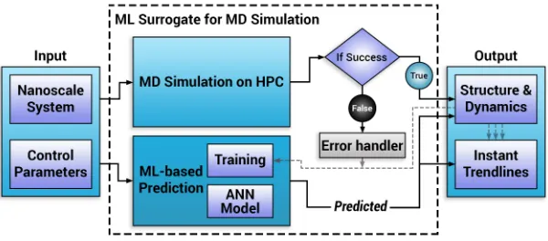
real-time and anyreal-time engagement with MD simulations, significantly enhancing the potential for their use in both education and research. The “ML surrogates for MD simulations” framework can be broadly defined as the approach to use ML to learn from MD simulations, and produce learned surrogates for MD simulations. Figure 2 shows the overview of this framework in the context of nanoscale materials engineering applications to predict the structure and/or dynamical properties (out-puts) characterizing the nanoscale system over a broad range of experimental control parameters (inputs). First, the attributes of the nanoscale system and the control parameters are fed to the framework (Figure 2). These inputs are used to launch the MD simulation on the HPC cluster. Simultaneously, these inputs are fed to the ML-based prediction module. Both the MD and ML methods are designed to extract (predict) the desired output quantities. Error handler aborts the MD simula-tion program and displays appropriate error messages when a simulation fails due to any pre-defined criteria. At the end of the simulation run, the output quantities are saved for future retraining of the ML model, which occurs after a set number of new successful simulation runs. After yielding a sufficiently large set of predictions, ML surrogate rapidly provides trendlines capturing the behavior of output quantities as a function of variation in input parameters.

ML surrogates for MD simulations can enable several capabilities which have particular significance in educa-tion: (i) learning pre-identified interesting features asso-ciated with the simulation outputs, (ii) almost instanta-neously generating accurate predictions for unsimulated state points, (iii) enabling anytime and anywhere access to simulation results, and iv) exhibiting auto-tunability with the ML model making increasingly accurate predic-tions after being trained on data from new simulapredic-tions.

nanocon-Fig. 2. System overview of the ML surrogate for MD simulation approach for generating rapid and accurate predictions associated with nanoscale phenomena for use in classroom teaching.

finement to illustrate the approach in further detail. Here, the goal is to extract the distribution of ions confined by two material surfaces represented as identical, uncharged parallel plates at z = −h/2 and z = h/2 (creating a confinement length of h). Here, the inputs include the nanoscale system of self-assembling electrolyte ions characterized by attributes such as valency and size, and the control parameters such as electrolyte concentration and interface separation. The outputs include the ionic density profiles or distribution functions in confinement. Our earlier work [5] showed that an ANN model can accurately predict 3 key output features: contact density, peak density, and mid-point density of confined ions. ANN outperformed other ML techniques such as polyno-mial regression, support vector regression, decision tree regression, and random forest regression. In this paper, we show that the ANN model can generate predictions for nearly all the desired features of the ionic density profile, producing almost the entire ionic distribution in excellent agreement with explicit MD simulation results.

A. Data Generation, Preparation, and Preprocessing

Prior domain experience and backward elimination using the adjusted R squared is used for selecting the most significant input parameters for creating the training data set. Using this process, five input parameters charac-terizing the ionic system are selected: confinement length

h, salt (electrolyte) concentrationc, positive ion valency

zp, negative ion valencyzn, and the ion diameterd. All

ions are assumed to have the same diameter; in general, oppositely charged ions have different sizes. The range of each parameter is selected as follows: h∈(3.0,4.0)

nm, c ∈ (0.3,0.9) M, zp ∈ 1,2,3, zn ∈ −1, and

d ∈ (0.5,0.75) nm. The salt concentration is defined as the number of negative ions per unit volume [2], [5]. Min-max normalization filter is applied to normalize the input data at the preprocessing stage.

The converged distribution for positive ions is selected as the output. The dataset created for investigations in

the earlier work [5] is reused. This dataset was generated by sweeping over a few discrete values for each of the input/output parameters to create and run 6,864 MD simulations utilizing HPC resources. On average, each MD simulation was performed for over≈5nanoseconds of ionic dynamics, and took 4200 CPU hours (≈36 min-utes per simulation with MPI/OpenMP parallelization). The training dataset creation took approximately 25 days including the queue wait times on the IU BigRed2 supercomputing cluster. The entire data set is separated into training and testing sets using a ratio of 0.8:0.2.

Each MD simulation produces positive ion distribution characterized by 300 points as output. For simplicity, using the symmetry of ionic density around the confine-ment centerz= 0, approximately half of the 300 points are selected as the output parameters. Accordingly, in the experiments that follow, ML is employed to make

P ≈150 predictions characterizing the density of ions in the left half of the confinement (withz∈(−h/2,0)). B. Feature Extraction and Regression

0.86 0.88 0.9 0.92 0.94 0.96 0.98 1

0 20 40 60 80 100 120

Success Rate

nth Prediction

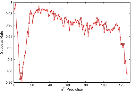
Fig. 3. Success rateAnassociated with thenth_{prediction made the} ML surrogate (Anis defined in Eq. 1).

IV. RESULTS

A. Validation of the ML approach

To validate the ML approach, we compare the training loss on training data and validation loss on test data to assess overfitting, and measure the success rate (or accuracy) associated with the ANN predictions on the test data. The training loss on 5491 simulations and validation loss (mean square error or MSE) on 1373 simulations decrease to 0.000194 and 0.000024 respec-tively within 4000 epochs of training. Similar reduction in training and validation losses indicates that the ML model is not overfitted.

Typically, in regression problems, accuracy or success rate is inherently not defined. To facilitate the compar-ison of ML predictions with MD results, we define a prediction as successful when the density value predicted by the ML surrogateρML_{is within the errorassociated} with the corresponding MD simulation estimate ρMD (ground truth). Accordingly, the average success rate or accuracy associated with the ML approach for the nth prediction (corresponding to thenth_{element in the output} set) is defined as:

An= 1

Ntest Ntest X

i=1

Θ

ρML_n,i−ρMD_n,i , n,i

(1)

where i indicates the simulation index, Ntest is the number of samples (simulations) in the test data, and

Θ(x, ) is a step function given by: Θ(x, ) = 1 for

x < , and Θ(x, ) = 0 for x ≥ . The overall ensemble-average success rate A of the ML prediction for the entire density profile can be estimated using

A = (1/P)PP

n=1An, where the sum is now over the

total number of predictionsP.

Figure 3 shows the success rate An associated with

thenth_{ML prediction for the testing dataset. In order for} the prediction to be well-evaluated,Anis only computed

for ML predictions associated with non-vanishing ρMD

(ρMD _{6= 0). In other words, results are not shown for}

≈ 20 output parameters (out of 150) where the ionic density and associated error from MD simulations are exactly 0 (regions near the left wall where finite-sized ions are prohibited from entering). As Figure 3 shows,

An is very good for all the evaluated ML predictions.

The ensemble-average success rate is found to be A= 0.958, and the lowest and highest recorded values for accuracy are An= 0.86 andAn= 0.997 respectively.

B. Ionic density profiles: comparing ML surrogate pre-dictions and MD simulations

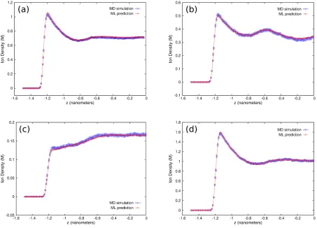
We now present plots of the positive ion density profiles showing the comparison between the predictions made by the ML surrogate and the results obtained from MD simulations. Results are shown for a set of 4 systems randomly selected from the entire testing dataset. These 4 systems are: system I (3.2, 1, -1, 0.6, 0.65), system II (3.6, 3, -1, 0.9, 0.75), system III (3.3, 3, -1, 0.35, 0.714), and system IV (3.6, 1, -1, 0.9, 0.6), where the parentheses list the 5 aforementioned input parameters characterizing the ionic system: confinement length h, positive ion valency zp, negative ion valency zn, salt

concentration c, and ion diameter d. Figure 4 (a) - (d) shows the ionic density profiles predicted by the ML surrogate for systems I, II, III, and IV respectively. As the figure indicates, for each system, the ML-predicted density profile is in excellent agreement with the result extracted using MD simulation (ground truth).

To make the comparison between ML predictions and MD simulation results more quantitative, we extract the overall accuracy of the ML prediction for each system (density profile). Similar to Eq. 1, we define this accuracy or success rateAiassociated with theithsystem

(simulation configuration) as:

Ai = 1

P

P

X

n=1

Θ ρML_n,i−ρMD_n,i

, n,i (2)

whereΘis the step function defined above, and the sum is now over the total number of predictionsPmade using the ML approach (as before, Ai is meaningful only at

non-zero ionic density values, makingP ≈130). Using Eq. 2, the success rates Ai for systems I, II, III, and

IV are found to be 0.98, 0.91, 0.78, 0.89 respectively. In addition to the good success rates, we point out that the ML inferences are made at a relatively much smaller time of≈0.2seconds compared to MD simulations (see below for further details).

C. Rapid access to trendlines using ML surrogates

Fig. 4. Ionic density profiles for systems I (a), II (b), III (c), and IV (d) predicted by ML surrogate (red circles) and extracted with MD simulation (blue squares) (see main text for system definitions).

much smaller “lookup time” for obtaining the ML infer-ences enable the generation of trendlines for the entire density profile almost instantaneously. Figures 5 and 6 show a selected subset of these ML-surrogate-predicted trendlines exhibiting the variation of ion distributions with changes in input parameters.

Figure 5 (a) and (b) shows the variation in the density of positive ions of valency zp = 1,2,3 at salt

con-centration c = 0.5 M and 0.9 M respectively. Other input parameters are fixed to h = 3.0 nm, zn = −1,

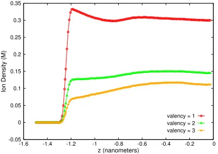
andd= 0.7 nm. The ML-generated trendlines are able to track distinct variations in density for different ion valencies and salinity conditions. The peak of the ionic density and the number of oscillations increase with c. Further, at a givenc, increasing the ion valency leads to the depletion of ions near the left surface (reduced ion density nearz= 0). Both these observations inferred by the ML surrogate follow the expected behavior in these systems as reported and elucidated in previous work [2]. Figure 6 shows ML-generated trendlines for systems that include parameters outside the dataset generated to train and test the ML model. Here, the density of positive ions of valency zp = 1,2,3 is predicted at a

salt concentration ofc= 0.1 M (other input parameters are the same as above). The depletion effects near the material surface (z = 0) due to stronger electrostatic interactions (e.g., at higher ion valencies) are expected to dominate at this relatively lower salt concentration. This is indeed borne out in the ML predictions which yield strong depletion of ions from the surface for divalent (zp = 2) and trivalent (zp = 3) ions, and

a relatively moderate enrichment near the surface for monovalent ions (zp = 1). An accurate assessment of

system behavior by the ML surrogate outside its training range shows its robustness and broad utility.

D. ML inference time and overall speedup

In the earlier paper, we introduced a simple formula illustrative of the possible gains or speedupS resulting from the use of scientific ML surrogates:

S= tsim

tp+ttr·Ntr/Np

, (3) where tsim is the time to run the MD simulation via

the sequential model,tp is the time it takes for the ML

Fig. 5. Trendlines for ionic density variation with positive ion valency at salt concentration (a)c= 0.5M and (b) 0.9 M. See main text for values of other input system parameters.

-0.05 0 0.05 0.1 0.15 0.2 0.25 0.3 0.35

-1.6 -1.4 -1.2 -1 -0.8 -0.6 -0.4 -0.2 0

Ion Density (M)

z (nanometers)

valency = 1 valency = 2 valency = 3

Fig. 6. Trendlines for ionic density variation with positive ion valency at salt concentrationc= 0.1M. This concentration is slightly outside the range of cemployed to train the ML model (0.3 - 0.9 M). See main text for values of other input system parameters.

one set of inputs, Np is the number of ML predictions

made, Ntr is the number of elements in the training

dataset, and ttr is the average walltime associated with

the MD simulation to create one of these elements.

Ntrttr represents the total time to create the training

dataset which includes the generation of the training data using MD simulations and the TensorFlow training time. In the specific case of the system of confined ions considered above, the training dataset consisted of 5491 simulation configurations (Ntr= 5491). The timettr to

generate one element of this training set is similar to the average runtime of the parallelized MD simulation. For the MD simulations considered in this work,tsim≈60

hours,ttr≈36 minutes, and ML inference timetp≈0.2

seconds. Comparing the run times of the parallelized MD simulation and the ML surrogate, we find that the ML surrogate yields output results over 10,000 (= ttr/tp)

times faster than parallel MD simulation. We also note that the ML surrogate is using 1 core to infer the result

as compared to 128 cores employed by the parallel simu-lation, indicating a complementary reduction in resource utilization by a factor of 128.

Given tp ttr and approximating tp → 0 in Eq.

3, we find S = SHPCNp/Ntr, where SHPC =tsim/ttr

is the traditional speedup obtained by parallelizing the MD simulation using HPC resources. We can identify the ML-only speedup as SML = Np/Ntr, i.e, the number

of predictions made by the ML surrogate divided by the size of the training dataset. The key feature of the ML-based approach is thus highlighted: S rises with increasing Np, that is, the speedup increases as the ML

surrogate is used to make more predictions. We also observe that for ML-enabled results to generate a “true” net speedup (S >1), the number of predictions made by the surrogate (ANN model) per one forward propagation must exceed Ntr/SHPC, that is, Np > Ntr/SHPC. For the example considered here,SHPC = 100, yielding the relation Np & 60. Considering this inequality, the use

of ML surrogate enhances the overall efficiency of the simulation framework when it predicts over 60 ionic density profiles. We note that the classroom use gives a natural increase inNp(andSML) by a factor proportional to the number of students in the class.

V. DISCUSSION ANDCONCLUSION

Future work will also explore the extent to which the learned ML surrogates can predict desired simulation outputs outside the pre-defined range of training datasets. Based on the aforementioned investigations, we pro-pose to design and integrate an ML surrogate with the current version of the “Ions in nanoconfinement” computational tool deployed on nanoHUB [3].1 _In ad-dition to executing MD simulations, we will introduce a method in the nanoHUB tool interface to predict the output density using ML surrogate. The ML-generated results will be shown as density profile plots on the user interface almost instantaneously. Based on the outcomes of this experiment, other nanoHUB tools designed by us will be explored for similar ML integration [20], [21].

While the results describing the utility of ML-integrated simulation framework are promising, exper-imentation with the use of these tools in classroom settings needs to be done. The use of the integrated ML-surrogate-MD-simulation framework will begin in Fall 2019 in an IU course (Simulating Nanoscale Systems) taught by the last author of this paper. We expect several of such tools to be utilized for classroom teaching over the next couple of years. Evaluation of the ML-integrated nanoHUB tools will be performed annually based on several feedback mechanisms including the test results and course questionnaires from classes where the tools will be used to teach course materials. Other feedback mechanisms include the reviews and questions asked on the nanoHUB webpage describing the tools.

ACKNOWLEDGMENT

This work is supported by the National Science Foun-dation under the Network for Computational Nanotech-nology (NCN) program through Award 1720625 (Net-work for Computational Nanotechnology - Engineered nanoBIO Node). Simulations were performed using the Big Red II supercomputing system supported in part by Lilly Endowment, Inc., through its support for the IU Pervasive Technology Institute, and in part by the Indiana METACyt Initiative. V.J. thanks P. Sharma for valuable comments on the manuscript.

REFERENCES

[1] R. Allen, J.-P. Hansen, and S. Melchionna, “Electrostatic poten-tial inside ionic solutions confined by dielectrics: a variational approach,” Phys. Chem. Chem. Phys., vol. 3, pp. 4177–4186, 2001.

[2] Y. Jing, V. Jadhao, J. W. Zwanikken, and M. Olvera de la Cruz, “Ionic structure in liquids confined by dielectric interfaces,”The

Journal of chemical physics, vol. 143, no. 19, p. 194508, 2015.

[3] K. Kadupitiya, S. Marru, G. C. Fox, and V. Jadhao, “Ions in nanoconfinement,” Dec 2017. [Online]. Available: https://nanohub.org/resources/nanoconfinement

[4] V. Jadhao, “Nanoscale simulations and engineering applications: Applications - self-assembly in nanoconfinement,” Feb 2019. [Online]. Available: https://nanohub.org/resources/29671

1_{The integrated tool is expected to be online in Fall 2019.}

[5] J. Kadupitiya, G. C. Fox, and V. Jadhao, “Machine learning for performance enhancement of molecular dynamics simula-tions,” in International Conference on Computational Science. Springer, 2019, pp. 116–130.

[6] V. Jadhao, F. J. Solis, and M. Olvera de la Cruz, “Simulation of charged systems in heterogeneous dielectric media via a true energy functional,” Phys. Rev. Lett., vol. 109, p. 223905, Nov 2012. [Online]. Available: http://link.aps.org/doi/10.1103/PhysRevLett.109.223905 [7] V. Jadhao, C. K. Thomas, and M. O. de la Cruz,

“Electrostatics-driven shape transitions in soft shells,”Proceedings of the

Na-tional Academy of Sciences, vol. 111, no. 35, pp. 12 673–12 678,

2014.

[8] S. C. Glotzer, “Assembly engineering: Materials design for the 21st century (2013 pv danckwerts lecture),”Chemical

Engineer-ing Science, vol. 121, pp. 3–9, 2015.

[9] V. Jadhao and M. O. Robbins, “Probing large viscosities in glass-formers with nonequilibrium simulations,” Proceedings of the

National Academy of Sciences, vol. 114, no. 30, pp. 7952–7957,

2017.

[10] N. E. Brunk and V. Jadhao, “Computational studies of shape con-trol of charged deformable nanocontainers,”Journal of Materials

Chemistry B, 2019.

[11] M. Spellings and S. C. Glotzer, “Machine learning for crystal identification and discovery,”AIChE Journal, vol. 64, no. 6, pp. 2198–2206, 2018.

[12] S. S. Schoenholz, “Combining machine learning and physics to understand glassy systems,”Journal of Physics: Conference

Series, vol. 1036, no. 1, p. 012021, 2018.

[13] V. Botu and R. Ramprasad, “Adaptive machine learning frame-work to accelerate ab initio molecular dynamics,”International

Journal of Quantum Chemistry, vol. 115, no. 16, pp. 1074–1083,

2015.

[14] A. L. Ferguson, “Machine learning and data science in soft materials engineering,” Journal of Physics: Condensed Matter, vol. 30, no. 4, p. 043002, 2017.

[15] K. Ch’ng, J. Carrasquilla, R. G. Melko, and E. Khatami, “Ma-chine learning phases of strongly correlated fermions,”Phys. Rev. X, vol. 7, p. 031038, Aug 2017.

[16] J. Kadupitiya, G. C. Fox, and V. Jadhao, “Machine learning for parameter auto-tuning in molecular dynamics simulations: Effi-cient dynamics of ions near polarizable nanoparticles,”Indiana

University, Nov, 2018.

[17] G. Fox, J. A. Glazier, J. Kadupitiya, V. Jadhao, M. Kim, J. Qiu, J. P. Sluka, E. Somogyi, M. Marathe, A. Adigaet al., “Learn-ing everywhere: Pervasive machine learn“Learn-ing for effective high-performance computation,” arXiv preprint arXiv:1902.10810, 2019.

[18] N. E. Brunk, M. Uchida, B. Lee, M. Fukuto, L. Yang, T. Douglas, and V. Jadhao, “Linker-mediated assembly of virus-like particles into ordered arrays via electrostatic control,” ACS Applied Bio

Materials, vol. 2, no. 5, pp. 2192–2201, 2019.

[19] G. Klimeck, M. McLennan, S. P. Brophy, G. B. A. III, and M. S. Lundstrom, “nanohub.org: Advancing education and research in nanotechnology,” Computing in Science Engineering, vol. 10, no. 5, pp. 17–23, Sept 2008.

[20] J. Kadupitiya, N. Brunk, S. Ali, G. C. Fox, and V. Jadhao, “Nanosphere electrostatics lab,” May 2018. [Online]. Available: https://nanohub.org/tools/nselectrostatic

[21] J. Kadupitiya, N. Brunk, M. Uchida, T. Douglas, and V. Jadhao, “Nanoparticle assembly lab,” January 2019. [Online]. Available: https://nanohub.org/tools/npassemblylab

[22] F. Cholletet al., “Keras,” 2015.