Exploratory methods for the study of incomplete and intersecting shape boundaries from landmark data

(1)

Research Article

Exploratory Methods for the Study of Incomplete and

Intersecting Shape Boundaries from Landmark Data

Fathi M. O. Hamed

1

and Robert G. Aykroyd

2 1_{University of Benghazi, Benghazi, Libya}

2_{University of Leeds, Leeds, UK}

Correspondence should be addressed to Robert G. Aykroyd; [email protected]

Received 25 July 2016; Revised 10 October 2016; Accepted 12 October 2016

Academic Editor: Z. D. Bai

Copyright © 2016 F. M. O. Hamed and R. G. Aykroyd. This is an open access article distributed under the Creative Commons Attribution License, which permits unrestricted use, distribution, and reproduction in any medium, provided the original work is properly cited.

Structured spatial point patterns appear in many applications within the natural sciences. The points often record the location of key features, called landmarks, on continuous object boundaries, such as anatomical features on a human face. In other situations, the points may simply be arbitrarily spaced marks along a smooth curve, such as on handwritten numbers. This paper proposes novel exploratory methods for the identification of structure within point datasets. In particular, points are linked together to form curves which estimate the original shape from which the points are the only recorded information. Nonparametric regression methods are applied to polar coordinate variables obtained from the point locations and periodic modelling allows closed curves to be fitted even when data are available on only part of the boundary. Further, the model allows discontinuities to be identified to describe rapid changes in the curves. These generalizations are particularly important when the points represent shapes which are occluded or are intersecting. A range of real-data examples is used to motivate the modelling and to illustrate the flexibility of the approach. The method successfully identifies the underlying structure and its output could also be used as the basis for further analysis.

1. Introduction

Many scientific investigations involve the recording of spa-tially located data. This data might summarize objects within an image as digitized versions of continuous curves. Once the data are collected often the original context is lost and the aim of the analysis is to identify which points are associated with each other and to link the points to reconstruct the original shape. These can then be seen as estimates of continuous curves and object outlines. If the original scene contains multiple structures, then the analysis must also divide the points into groups with separate curves used to describe the points in each group. It is important to note that this is likely to form only the first part of an analysis and hence can be seen as exploratory data analysis.

This paper looks at the use of smoothing splines to identify and describe geometric patterns in sets of points. It is assumed that the points lie on smooth curves but that a dataset may contain multiple intersecting curves. It is vital that this be done in a nonparametric way so that the widest

possible range of patterns can be highlighted. In general, these are closed, or nearly closed, curves and so a transformation to polar coordinates is used to simplify the analysis. Intersecting curves are described by allowing discontinuities in the fitted curves. These procedures are illustrated using simulated data and varied real datasets describing human faces, gorilla skulls, handwritten number 3’s, and an archaeological site. These provide a wide variety of point patterns and reinforce the gen-eral usefulness of the proposed methods. For mathematical detailed description and applications of shape-based analysis of points, refer to, for example, Batschelet [1], Bookstein [2], Dryden and Mardia [3], and Lele and Richtsmeier [4].

To allow for this wide variety of possible curves a nonparametric fitting approach, such as splines, can be used (see, e.g., [5, 6]). The flexibility is helpful in the exploratory statistical analysis of a dataset, and the results can be used to suggest parametric equations for later analysis. Nonpara-metric regression is the general name for a range of curve fitting techniques which make few a priori assumptions about the true shape. In nonparametric regression, several different Volume 2016, Article ID 1285026, 9 pages

(2)

families of basis functions can be used to describe curves; one of the common kinds of basis for smooth curves is the spline. Splines are generally defined as piecewise polynomials in which curve, or line, segments are joined together to form a continuous function. The spline smoothing approach to nonparametric regression is discussed, for example, by Silverman [7] and extended to deal with branching curves by defining a roughness penalty by Silverman and Wood [8]. For an introduction to natural cubic spline see Green and Silverman [9]. For more review of spline methods in statistics see Wegman and Wright [10], Silverman [11], Silverman [7], Nychka [12], and Wahba [13].

It is important to note that there are many existing gen-eral frameworks for performing spline-based regression. For example, multivariate adaptive regression splines (MARS) [14] or its more robust generalizations, RMARS [15] and RCMARS [16], with a good overview and comparison in [17]. These follow the general approach of general additive modelling [18] and give a formal framework for fitting and model selection.

A brief introduction to splines, along with the extension to circular data, is given in Section 2. The main results of this paper are given in Section 3 by considering modelling for single curves with occlusions and multiple intersecting curves. Although simulated examples are used to illustrate, the main real-data examples are given in Section 4. General discussion appears in Section 5.

2. Nonparametric Curve

Estimation and Periodic Splines

A smoothing spline is a nonparametric curve estimator that is defined as the solution to a minimization problem. It provides a flexible smooth function for situations in which a simple polynomial or nonlinear regression model is not suitable. For

a set of𝑛observations𝜒 = {(𝑥_𝑖, 𝑦_𝑖), 𝑖 = 1, 2, . . . , 𝑛}consider

a regression problem where the observations are assumed to satisfy

𝑦_𝑖= 𝑓 (𝑥_𝑖) + 𝜖_𝑖, 𝑖 = 1, 2, . . . , 𝑛, (1)

where the errors 𝜖_𝑖 are uncorrelated with zero mean and

constant variance, 𝜎2. Then the spline smoothing method

uses the data to construct a curve 𝑓 by minimizing the

objective function

𝐽 (𝑓; 𝜒, 𝜆) =1 𝑛

𝑛

∑

𝑖=1

(𝑦_𝑖− 𝑓 (𝑥_𝑖))2

+ 𝜆 ∫−∞

∞ (𝑓

(𝑚)_(𝑥))2_𝑑𝑥,

(2)

where 𝑓(𝑚) represents the 𝑚th derivative of 𝑓, with 𝑚

being a positive integer, and 𝜆 is a smoothing parameter.

For more details of smoothing splines see, for example, Eubank [19], Eubank [6], and Cantoni and Hastie [20]. An alternative definition of the level of smoothing is in terms

of anequivalent degrees of freedom,Df, which describes the

amount of information in the data needed to estimate the

residuals. The functionsmooth.spline[21] allows𝜆orDfto

be specified, but the degrees of freedom have been used in what follows as this gives a more intuitive interpretation.

The above objective function consists of two parts: the first measures the agreement of the function and the data and the second is a roughness penalty reflecting the total curvature—this can also be interpreted in a Bayesian setting

as the likelihood and prior. Hence, for givenDf, the estimate

of𝑓is given by

̂𝑓 (𝑥,Df) =min

𝑓 𝐽 (𝑓; 𝜒,Df) , 𝑥 ∈R. (3)

IfDfis large then the function is rough but closely fits the

data, whereas whenDfis small then the function is smooth

but may not fit the data well. Here the choice ofDfis made

automatically using standard leave-one-out cross-validation [22]; that is,

̂

Df=min Df

𝑛

∑

𝑖=1

(𝑦_𝑖− ̂𝑓−𝑖(𝑥_𝑖,Df))2, (4)

wherê𝑓−𝑖(⋅,Df)is the fitted spline curve, for given parameter

Df, and with the𝑖th data point,(𝑥_𝑖, 𝑦_𝑖), being removed. Then

̂𝑓(⋅, ̂Df)is the fitted curve using the cross-validation estimate of the degrees of freedom.

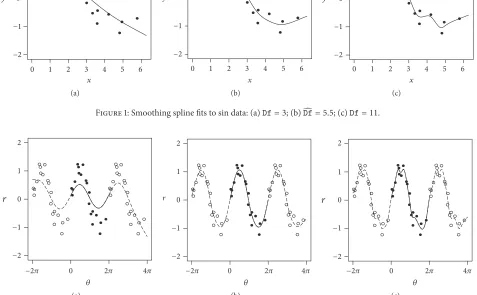
Figure 1 shows fitted curves using splines with different

degrees of freedom,Df. The true curve is a sine function with

noise level𝜎 = 1/4which corresponds to a signal to noise

ratio (SNR= 𝜎𝑓/𝜎) of about 2. In (a) Dfis about half the

value found using cross-validation which is used in (b), with (c) using double the cross-validation degrees of freedom. The small degrees-of-freedom value gives a smoother fitted curve that ignores many of the points in the data whereas a large value produces a rougher fit which more closely follows the

data. The automatic choice waŝDf= 5.5which gives a very

good fit to the data reproducing the sin curve well.

For this dataset, the periodic nature of the sin function has, so far, been ignored, and it is clear that the extreme left and right do not match exactly. For such datasets, made up of angles or directions, ignoring the periodic nature of the measurements when smoothing may produce unacceptable edge effects. A simple approach for dealing with this issue will now be considered.

Suppose that the dataset is made up of paired angles and

distances which will be denoted as𝜗 = {(𝜃_𝑖, 𝑟_𝑖) : 𝑖 = 1, . . . , 𝑛}

for a sample of size𝑛. A simple approach for periodic data

measured in the interval(0, 2𝜋), say, is to repeat the data.

That is, for each angle 𝜃_𝑖, the corresponding new angular

values are(𝜃_𝑖− 𝑝𝜋, . . . , 𝜃_𝑖− 𝜋, 𝜓, 𝜃_𝑖+ 𝜋, . . . , 𝜃_𝑖+ 𝑝𝜋), where

𝑝 = 1, 2, . . ., and similarly repeat the corresponding radial

distances𝑟_𝑖 to be(𝑟_𝑖, . . . , 𝑟_𝑖). This produces a dataset, 𝜗𝑝 =

{(𝜃_𝑖, 𝑟_𝑖) : 𝑖 = 1, . . . , 𝑛󸀠_}_{, with}_𝑛󸀠 _{= (2𝑝 + 1) × 𝑛}_{data values,}

and even for small𝑝 (e.g.,𝑝 = 1 or 2) this gives a very

good approximation to the full periodic spline. Cogburn and Davis [23] present the theory of periodic smoothing spline with application to the estimation of periodic functions and

the R functionperiodicSplinefrom the packagesplines

(3)

y 2

1

0

−1

−2

1 2 3 4 5 6

0

x (a)

0 1 2 3 4 5 6

x y

2

1

0

−1

−2

(b)

0 1 2 3 4 5 6

x 2

1

0 y

−1

−2

[image:3.600.79.536.70.235.2]

(c)

Figure 1: Smoothing spline fits to sin data: (a)Df= 3; (b)̂Df= 5.5; (c)Df= 11.

r 2

1

0

−1

−2

0

−2𝜋 2𝜋 4𝜋

𝜃

(a)

2

1

0 r

−1

−2

0 2𝜋 4𝜋

−2𝜋

𝜃

(b)

r

0 2

1

0

−1

−2

−2𝜋 2𝜋 4𝜋

𝜃

[image:3.600.62.539.137.432.2]

(c)

Figure 2: Periodic spline fits to sin data: (a)Df= 7; (b)DfCV= 15; (c)Df= 30.

As illustration consider Figure 2 which shows fitted

curves equivalent to those in Figure 1 but with𝑝 = 1. The solid

circles are the original data with open circles representing the copied data points. Similarly, the solid line is the spline fitted curve over the original interval with the dashed line showing the fitted curve over the copied data points. In all cases the fit is better than in Figure 1, with the periodic nature, reproduced well, and as before the cross-validation choice of smoothing has produced an excellent reconstruction of the true sin curve.

Once fitted a residual sum of squares, RSS, calculated on the original data values, can be used as a measure of goodness-of-fit. Here this will be calculated using the radial distances with definition

RSS=

𝑛

∑

𝑖=1

(𝑟_𝑖− ̂𝑟 (𝜃_𝑖, ̂Df))2 (5)

but other versions could be used, for example, the Euclidean distance between fitted and observed points.

Of course, the approach could lead to a poor fit if the data is not periodic, but to prevent this it is possible to allow for a discontinuity in the relationship. Here the approach of Gu

[24], who considered discontinuities in cubic splines with a jump at a known location, will be extended to the periodic case and with an unknown discontinuity location.

Suppose that the points𝜗 = {(𝑟_𝑖, 𝜃_𝑖) : 𝑖 = 1, . . . , 𝑛}are

partitioned into two groups with the first,𝜗₁, containing all

the points with angles up to and including the change point

and𝜗₂those with angles above. Assuming that the points are

ordered in increasing value of the angle, so that𝜃₁≤ ⋅ ⋅ ⋅ ≤ 𝜃_𝑛,

then let𝜗₁ = {(𝜃_𝑖, 𝑟_𝑖); 𝑖 = 1, . . . , 𝑘}be the data before the

change point and𝜗₂= {(𝜃_𝑖, 𝑟_𝑖); 𝑖 = 𝑘+1, . . . , 𝑛}the remaining

data. For change point at𝜃_𝑘two curves are fitted to the data

such that

̂𝑟 (𝜃, ̂Df) ={_{

{

min_𝑟 𝐽 (𝑟; 𝜗₁, ̂Df1) , for𝜃 ≤ 𝜃𝑘

min_𝑟 𝐽 (𝑟; 𝜗₂, ̂Df2) , for𝜃 > 𝜃𝑘,

(6)

where cross-validation is used separately on the two parts

leading to two degrees of freedom, ̂Df= (̂Df1, ̂Df2). The

significance of the change point could be assessed through a chi-squared test, but here a change point influence graph is considered based on the goodness-of-fit.

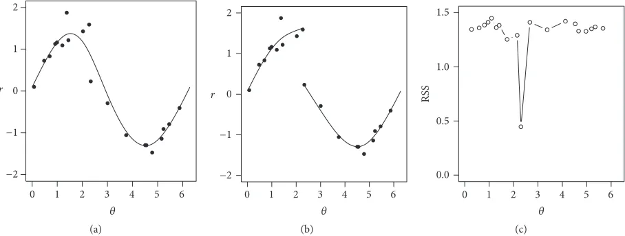
Consider the sin data shown in Figure 3(a) which has a

(4)

0 1 2 3 4 5 6 r

2

1

0

−1

−2

𝜃

(a)

r 2

1

0

−1

−2

0 1 2 3 4 5 6

𝜃

(b)

RSS

0 1 2 3 4 5 6

𝜃

1.5

1.0

0.5

0.0

(c)

Figure 3: (a) Data from sin function with a discontinuity; (b) best two-part curve; (c) residual sum of square for two-part curves.

The curve in Figure 3(a) is fitted using a smoothing spline, but ignoring the change point, it is possible that the curves in Fig-ure 3(b) are fitted using smoothing splines with change point at the estimated location. The automatically chosen value for

the degrees of freedom,̂Df, for the single curve in (a) is14.5

whereas for the two-part curve the overall degrees of freedom

are ̂Df1+ ̂Df2= 11. Figure 3(c) shows the residual sum of

squares, RSS, for each possible change point location with a very clear minimum. The RSS for the curve in Figure 3(a) is

1.3while, in (b), it has reduced to0.45, which is substantially

smaller and provides a much better description of the data. Hence this approach provides an intuitive approach to finding change points in data automatically.

3. A Model for Multiple Overlapping Curves

3.1. Motivation. To motivate the modelling, consider an unobserved true scene containing a few objects of various shape and sizes, with possible overlap. However, instead of the scene being recorded faithfully, only partial information is taken and, in particular, only points along the edges of the objects are recorded. These points might be chosen to identify features with special significance or they might simply be at equal or random locations along the edge. Further, due to overlaps, points from the full edge may not be in the dataset. Once collected, there is no record of which points are from which object, and no record is kept of possible object shapes nor even the number of objects. Hence, let the dataset consists

of a collection of 𝑛points,𝜒 = {(𝑥_𝑖, 𝑦_𝑦) : 𝑖 = 1, . . . , 𝑛},

recorded within some small region in 2D.

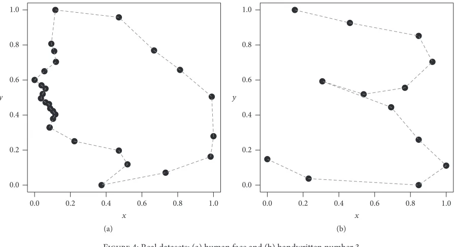
Figure 4 shows example datasets which will be analysed later. Panel (a) shows a human face profile with the forehead, eyes, nose, mouth, and chin clearly identifiable on the left— the points on the right locate the back of the neck and the hairline. Panel (b) shows points located along a handwritten number 3 at approximately equally spaced intervals.

3.2. Modelling a Single Curve with Occlusion. Before the peri-odic smoothing spline approach can be applied it is necessary

for the data to be first transformed to polar coordinates.

First define acentre,(𝜉, 𝜁), which can be estimated using the

data centroid(̂𝜉, ̂𝜁) = (𝑥, 𝑦) and then use the one-to-one

transformation

𝑟_𝑖= ((𝑥_𝑖− 𝑥)2+ (𝑦_𝑖− 𝑦)2)1/2,

𝜃_𝑖=tan−1((𝑦𝑖− 𝑦)

(𝑥_𝑖− 𝑥)) ,

𝑖 = 1, . . . , 𝑛.

(7)

This gives rise to an alternative data representation via the

centre(𝑥, 𝑦)and polar coordinates𝜑 = {(𝑟_𝑖, 𝜃_𝑖) : 𝑖 = 1, . . . , 𝑛}.

Note that although this representation contains𝑛+2pieces of

information, by construction, the polar coordinate variables are not independent. Of course, other estimates of centre could be considered, such as the point which minimizes the variance of the radii. In particular, this measure should be more robust to presence of occlusions.

To illustrate the transformation and the subsequent spline smoothing consider the simulated data in Figure 5. Panel (a) shows the given points along with the sample centre marked with a “+”; the points in (b) are the corresponding polar coordinates relative to this centre. Also shown in (b) are the nonperiodic smoothing spline (continuous black line) and the period smoothing spline (dashed red line). These are all closely aligned except at the extreme angles. Once transformed back into Cartesian coordinates, as shown in panel (c), the slight discrepancies between the fitted splines are more clearly visible. At the far right of the plot, the periodic spline curve is closed and more naturally represents a possible object, whereas the nonperiodic spline is not closed making it difficult to interpret if this were part of the edge of a real object.

[image:4.600.73.527.74.246.2]

(5)

y 1.0

0.8

0.6

0.4

0.2

0.0

0.2 0.4 0.6 0.8 1.0

0.0

x (a)

y 1.0

0.8

0.6

0.4

0.2

0.0

0.2 0.4 0.6 0.8 1.0

0.0

[image:5.600.71.519.71.314.2]

x (b)

Figure 4: Real datasets: (a) human face and (b) handwritten number 3.

+

x

3 2 1 0 −1 −2 −3 y

3

2

1

0

−1

−2

−3

(a)

r

−𝜋 −𝜋/2 0 𝜋/2 𝜋

𝜃 4.0

3.5

3.0

2.5

2.0

1.5

1.0

(b)

x

y ₊

3 2 1 0 −1 −2 −3 3

2

1

0

−1

−2

−3

(c)

Figure 5: (a) Simulated data; (b) polar coordinate data with fitted spline curve; (c) data with back-transformed fitted curves. In (b) and (c) the solid curves use standard splines, whereas the dashed use the periodic spline.

+

x 1 2 3

0 −1 −2 −3 y

3

2

1

0

−1

−2

−3

(a)

−𝜋 −𝜋/2 0 𝜋/2 𝜋

𝜃 r

4.0

3.5

3.0

2.5

2.0

1.5

1.0

(b)

x

y +

3 2 1 0 −1 −2 −3 3

2

1

0

−1

−2

−3

(c)

[image:5.600.63.536.331.497.2] [image:5.600.64.540.540.706.2]

(6)

fitted curves are transformed back into Cartesian coordinates, as shown in panel (c). The periodic smoothing spline has done a very good job of interpolating the missing part of the curve and the results can easily be relied upon in further analysis. In particular, slight changes in the position of a few critical point will lead to very different shapes for the nonperiodic spline.

To summarize, application of smoothing splines to peri-odic point data has proved very successful. The modification of the duplicated data is a simple, yet effective way to create closed curves and to interpolate where data are missing. The approach has provided a robust and informative reconstruc-tion of the unknown curve from the data.

3.3. Modelling Multiple Intersecting Curves. To allow for inter-secting and overlapping curves the points are partitioned into

𝑚groups,𝑆_𝑗, where𝑗 = 1, 2, . . . , 𝑚. That is,𝑆_𝑗 ⊆ (1, . . . , 𝑛)

with𝑆_𝑖∩ 𝑆_𝑗 = 0when𝑖 ̸= 𝑗and𝑆₁∪ ⋅ ⋅ ⋅ ∪ 𝑆_𝑚= (1, . . . , 𝑛). To

record group membership a matrix𝑊_𝑛×𝑚 = (𝑤_𝑖𝑗)is defined,

where𝑤_𝑖𝑗= 1if point𝑖belongs to group𝑗 (𝑖 ∈ 𝑆_𝑗)and𝑤_𝑖𝑗= 0

otherwise. Then,∑_𝑗𝑤_𝑖𝑗 = 1and ∑_𝑖𝑤_𝑖𝑗 = 𝑛_𝑗, where𝑛_𝑗 is

the number of points in the𝑗th group; that is,𝑛_𝑗 = |𝑆_𝑗|. For

each group, working in polar coordinates, there is a centre,

(𝜉_𝑗, 𝜁_𝑗), and coordinates relative to the centre,𝜗_𝑗= {(𝑟_𝑖𝑗, 𝜃_𝑖𝑗) :

𝑖 = 1, . . . , 𝑛_𝑗}, with the full set of parameters denoted as𝜗 =

{𝜗_𝑗 : 𝑗 = 1, . . . , 𝑚}. The corresponding Cartesian coordinates

can be written asΓ_𝑗= {(𝜇_𝑖𝑗,]_𝑖𝑗) : 𝑖 = 1, . . . , 𝑛_𝑗}, with

𝜇_𝑖𝑗= 𝜉_𝑗+ 𝑟_𝑖𝑗cos(𝜃_𝑖𝑗) ,

]_𝑖𝑗= 𝜁_𝑗+ 𝑟_𝑖𝑗sin(𝜃_𝑖𝑗) ,

for𝑖 = 1, . . . , 𝑛_𝑗, 𝑗 = 1, . . . , 𝑚, (8)

and the full collection of data asΓ = {Γ_𝑗 : 𝑗 = 1, . . . , 𝑚}.

Further, it is assumed that the point locations are recorded with error giving observed measurements

𝑥_𝑖𝑗= 𝜇_𝑖𝑗+ 𝜖_𝑖𝑗, 𝑦_𝑖𝑗=]_𝑖𝑗+ 𝜀_𝑖𝑗,

for𝑖 = 1, . . . , 𝑛_𝑗, 𝑗 = 1, . . . , 𝑚, (9)

where𝜖 and𝜀are independent Gaussian random variables

with zero mean and constant variance𝜎2.

In what follows the full dataset will, without further

explanation, be referred to using either𝜒 = {(𝑥_𝑖𝑗, 𝑦_𝑖𝑗) : 𝑖 =

1, . . . , 𝑛_𝑗, 𝑗 = 1, . . . , 𝑚}and𝜗 = {(𝜃_𝑖𝑗, 𝑟_𝑖𝑗) : 𝑖 = 1, . . . , 𝑛_𝑗, 𝑗 =

1, . . . , 𝑚} or equivalently, but without explicit reference to

the group membership, 𝜒 = {(𝑥_𝑖, 𝑦_𝑖) : 𝑖 = 1, . . . , 𝑛}and

𝜗 = {(𝜃𝑖, 𝑟𝑖) : 𝑖 = 1, . . . , 𝑛}as is most convenient and intuitive.

3.4. Estimation with Multiple Intersecting Curves. Now con-sider estimation of the model unknowns from observed data. Start by supposing that a dataset is available but that the group

membership information is intact; then the group centres could be estimated as

̂𝜉𝑗 = 𝑥𝑗=

∑𝑛_𝑖=1𝑤_𝑖𝑗𝑥_𝑖 ∑_𝑖𝑤_𝑖𝑗 ,

̂𝜁𝑗 = 𝑦𝑗 =

∑𝑛_𝑖=1𝑤_𝑖𝑗𝑦_𝑖 ∑_𝑖𝑤_𝑖𝑗

(10)

and, although some of these are unimportant, corresponding

polar coordinate representation of point𝑖relative to group

centre𝑗is

̂𝑟𝑖𝑗= ((𝑥𝑖− 𝑥𝑗)2+ (𝑦𝑖− 𝑦𝑗) 2

)1/2, (11)

̂𝜃_𝑖𝑗=tan−1(𝑦𝑖− 𝑦𝑗

𝑥_𝑖− 𝑥_𝑗) , (12)

where𝑖 = 1, . . . , 𝑛and𝑗 = 1, . . . , 𝑚. The overall residual sum

of squares is then the sum of the separate components

RSS=

𝑚

∑

𝑗=1

RSS_𝑗=

𝑚

∑

𝑗=1 𝑛𝑗

∑

𝑖=1(𝑟𝑖𝑗− ̂𝑟 (𝜃𝑖𝑗, ̂Df𝑗)) 2

. (13)

Now consider the case when the group membership is unknown and must be inferred from the data. The aim is to find linked points by fitting curves. Some datasets have more than one curve and some have intersecting curves. Then classifying the points into groups may help to fit the correct curves that represent the data.

In general, this can be thought of as a change point prob-lem, as already discussed, to address the lack of stationarity in the values. A change point occurs at some point in the data if all of the values up to and including it share a common curve while all those after the change point share another. This is exactly the same situation as the discussion in Section 2 and hence the same method of solution is applied.

4. Application to Real Data

4.1. General. The previous sections have illustrated the pro-posed exploratory data analysis tools on simulated example, whereas in this section the success of the approach is demonstrated on a varied range of real datasets. There is no wish to construct formal equations to define the shape but to stimulate further analyses.

(7)

x y

5

4

3

2

1

0

3.5 3.0 2.5 2.0 1.5 1.0

(a)

−𝜋 −𝜋/2 0 𝜋/2 𝜋

3.0

2.5

2.0

1.5

1.0

0.5

(b)

+ 5

4

3

2

1

0

4.0 3.5 3.0 2.5 2.0 1.5 1.0 0.5

(c)

Figure 7: (a) Face data; (b) polar coordinate data with fitted spline curves; (c) back-transformed fitted curves. In (b) and (c) the solid curves use standard splines, whereas the dotted use periodic splines.

(a)

−𝜋 −𝜋/2 0 𝜋/2 𝜋

140

120

100

80

60

40

(b)

+

0 50 100

200 150 100 50 0 −50

(c)

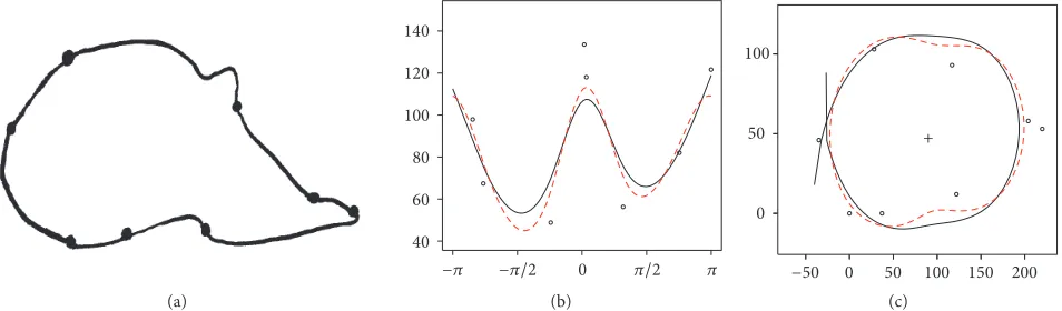
Figure 8: (a) Schematic diagram of a gorilla skull with anatomical landmarks for a male gorilla; (b) landmarks in polar coordinate and spline curves; (c) landmarks along with back-transformed fitted spline curves. In (b) and (c) the solid curves use standard splines, whereas the dotted use the periodic spline.

the standard smoothing splines. Both produce well fitted curves for the face. It is worth noting that the fitted curve can be evaluated at arbitrarily close locations, not only at the data points, and hence a smoothly interpolated curve can be drawn.

4.3. Example 2: Gorilla Skulls. This dataset, taken from Dry-den and Mardia [3], is composed of 8 anatomical landmarks from the skulls of 29 male and 30 female gorillas. A landmark

is defined asa point of correspondence on each object that

matches between and within populations [3]. Figure 8(a) shows a schematic diagram of a typical skull with the landmarks indicated.

Figure 8(c) shows landmarks for one of the male gorillas and Figure 8(b) the corresponding points in polar coordi-nates along with spline fitting to the dataset and in Figure 8(c) after back-transforming. For both, the fits are good but at the expense of low smoothing in the spline. This fitting procedure was repeated for the other gorilla skulls and surprisingly the smoothed curves give good summaries allowing the skulls to be easily categorised into four main groups covering mainly male skulls which are rather elongated and two covering mainly female skulls which appear more rounded. The males

lead to generally larger values of the degrees of freedom (6 <Df< 8) than the females (Df≈ 2). In fact, the automatic choice of the degrees-of-freedom parameter can be used as a simple discrimination variable giving only 8 out of 59 incorrectly classified skulls. It is important to note that this was not a preconceived discriminator but was identified by the exploratory analysis. This has highlighted the usefulness of simple and flexible tools as a preliminary step in a more wide-ranging investigation.

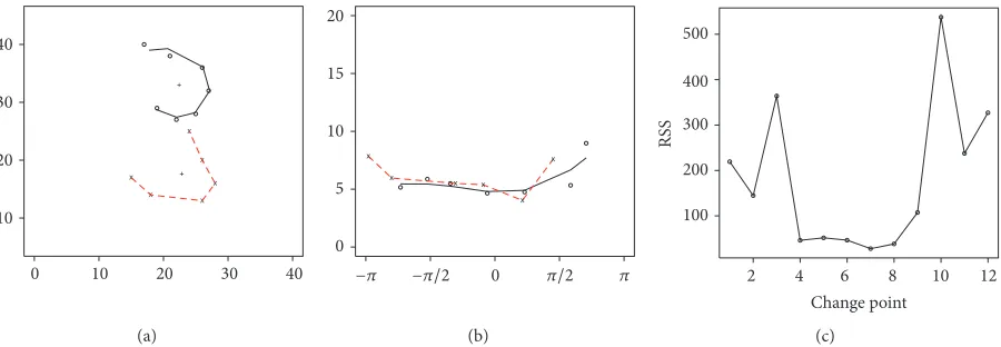
4.4. Example 3: The Number 3. Another dataset, again taken from Dryden and Mardia [3], is made up of 13 landmarks from 30 handwritten number 3’s; see Figure 9(a). Suppose the

data are divided into two subsets with𝑛₁and𝑛₂observations,

[image:7.600.83.520.71.223.2] [image:7.600.67.544.273.413.2]

(8)

0 40

30

20

10

10 20 30 40

(a)

20

15

10

5

0

−𝜋 −𝜋/2 0 𝜋/2 𝜋

(b)

Change point

RSS

12 10 8 6 4 2 500

400

300

200

100

(c)

Figure 9: (a) A typicalnumber 3dataset along with the back-transformed fitted two-part spline; (b) points in polar coordinates and two-part spline curve; (c) RSS plotted against change point position.

(a)

+ +

0.04 0.06 0.08

0.02

0.00

0.25 0.24 0.23 0.22 0.21

(b)

−𝜋 −𝜋/2 0 𝜋/2 𝜋

0.04

0.03

0.02

0.01

0.00

(c)

Figure 10: (a) Magnetic survey data for part of an iron-age archaeological site; (b) selected pits along with back-transformed fitted two-part spline curve; (c) polar coordinates and fitted two-part spline curve.

4.5. Example 4: Archaeological Site Data. The data in Fig-ure 10(a) shows part of a typical image dataset (supplied by Alistair Marshall of the Guiting Power Amenity Trust; see Aykroyd et al. [26] for details) from a magnetic survey of an archaeological site. As well as linear features, which represent ditches, there are also several drifts of pits, but blurring and noise tend to camouflage the exact locations. Panel (b) shows the locations of some of these pits, appearing as small circles, and panel (c) shows the corresponding polar coordinates relative to the two data centres (marked “+” in (b)). According to the minimum value of the residual sum of squares, RSS, the observations can be classified automatically into two groups. The data centres are calculated for each subset, the small

circles are the data in the first subset, and “×” are the

data in the second subset, with the fitted curves plotted in Figure 10(c). Then the fitted curves are back-transformed into Cartesian coordinate as shown in panel (b). The solid curve is for the first subset while the dotted curve is for the second subset. The aim of the analysis is to identify which points are associated with each other and to fit curves to the points, and this has been achieved well. The resulting linked points might then form part of further analysis or aid physical excavation.

5. Discussion

[image:8.600.76.526.71.227.2] [image:8.600.67.532.274.415.2]

(9)

There is scope for extending the approach to include larger numbers of curves where it is not possible to divide the curves with a single change point. The nature of the problem is closely related to classification where the group membership is missing. This strongly suggests that a prob-abilistic approach might be considered based on statistical distribution models. This would then fit into the general framework where the EM algorithm has proven very useful. Also, there is a need to extend the approach to deal with unordered points and ones which are not star-shaped. These are areas of possible future work. Further, it is of interest to develop a similar procedure which would allow more formal modelling and model section, perhaps following the approach of general additive modelling [18].

The applications are various and varied with an illustra-tive example of the method when the data points are anatomi-cal landmarks defined by geometrianatomi-cal features, equally spaced but blindly placed points along smooth curves and from extreme intensity points in grey-scale images. Further, the results of the analysis have provided new variables which could be the starting point for other analyses. Hence there is potential for this to be a valuable exploratory data analysis method in the tool-kit of applied statisticians and applied scientists.

Competing Interests

The authors declare that there is no conflict of interests regarding the publication of this paper.

References

[1] E. Batschelet, Circular Statistics in Biology, Academic Press, London, UK, 1981.

[2] F. L. Bookstein,Morphometric Tools for Landmark Data: Geom-etry and Biology, Cambridge Univesity Press, Cambridge, UK, 1991.

[3] I. L. Dryden and K. V. Mardia,Statistical Shape Analysis, Wiley Series in Probability and Statistics: Probability and Statistics, John Wiley & Sons, Chichester, UK, 1998.

[4] S. Lele and J. Richtsmeier,An Invariant Approach to Statistical Analysis of Shapes, Chapman & Hall/CRC, 2001.

[5] T. P. Ryan,Modern Regression Methods, Wiley Series in Prob-ability and Statistics: Applied ProbProb-ability and Statistics, John Wiley & Sons, New York, NY, USA, 1997.

[6] R. L. Eubank,Nonparametric Regression and Spline Smoothing, Marcel Dekker, New York, NY, USA, 1999.

[7] B. W. Silverman, “Some aspects of the spline smoothing approach to nonparametric regression curve fitting,”Journal of the Royal Statistical Society B, vol. 47, no. 1, pp. 1–52, 1985. [8] B. W. Silverman and J. T. Wood, “The nonparametric estimation

of branching curves,”Journal of the American Statistical Associ-ation, vol. 82, no. 398, pp. 551–558, 1987.

[9] P. J. Green and B. W. Silverman, Non Parametric Regression and Generalized Linear Models: A Roughness Penalty Approach, Chapman and Hall, 1994.

[10] E. J. Wegman and I. W. Wright, “Splines in statistics,”Journal of the American Statistical Association, vol. 78, no. 382, pp. 351–365, 1983.

[11] B. W. Silverman, “A fast and efficient cross-validation method for smoothing parameter choice in spline regression,”Journal of the American Statistical Association, vol. 79, no. 387, pp. 584– 589, 1984.

[12] D. Nychka, “Splines as local smoothers,”The Annals of Statistics, vol. 23, no. 4, pp. 1175–1197, 1995.

[13] G. Wahba, “Splines in nonparametric regression,” in Encyclope-dia of Environmetrics, John Wiley & Sons, New York, NY, USA, 2006.

[14] J. H. Friedman, “Multivariate adaptive regression splines,”The Annals of Statistics, vol. 19, pp. 1–67, 1991.

[15] A. ¨Ozmen and G. W. Weber, “RMARS: robustification of mul-tivariate adaptive regression spline under polyhedral uncer-tainty,”Journal of Computational and Applied Mathematics, vol. 259, pp. 914–924, 2014.

[16] A. ¨Ozmen, G. W. Weber, I. Batmaz, and E. Kropat, “RCMARS: robustication of CMARS with different scenarios under polyhe-dral uncertainty set,”Communications in Nonlinear Science and Numerical Simulation, vol. 16, pp. 1780–1787, 2011.

[17] A. ¨Ozmen,Robust Optimization of Spline Models and Complex Regulatory Networks, Contributions to Management Science, Springer, 2016.

[18] T. J. Hastie and R. J. Tibshirani,Generalized Additive Models, Chapman & Hall/CRC, 1990.

[19] R. L. Eubank, “Diagnostics for smoothing splines,”Journal of the Royal Statistical Society. Series B. Methodological, vol. 47, no. 2, pp. 332–341, 1985.

[20] E. Cantoni and T. Hastie, “Degrees-of-freedom tests for smoothing splines,”Biometrika, vol. 89, no. 2, pp. 251–263, 2002. [21] R Core Team,R: A Language and Environment for Statistical Computing,, R Foundation for Statistical Computing, Vienna, Austria, 2016, http://www.R-project.org/.

[22] P. Craven and G. Wahba, “Smoothing noisy data with spline functions: estimating the correct degree of smoothing by the method of generalized cross-validation,”Numerical Mathemat-ics, vol. 31, pp. 377–403, 1979.

[23] R. Cogburn and H. T. Davis, “Periodic splines and spectral estimation,”The Annals of Statistics, vol. 2, pp. 1108–1126, 1974. [24] C. Gu, “Multivariate spline regression,” in Smoothing and

Regression: Approaches, Computation and Application, M. G. Schimek, Ed., pp. 329–354, John Wiley & Sons, New York, NY, USA, 2000.

[25] R. J. Morris, J. T. Kent, K. V. Mardia, R. G. Aykroyd, M. Fidrich, and A. Linney,Exploratory Analysis of Facial Growth, Leeds University Press, 1999.

[26] R. G. Aykroyd, J. G. Haigh, and G. T. Allum, “Bayesian methods applied to survey data from archeological magnetometry,”

(10)

Submit your manuscripts at

http://www.hindawi.com

Hindawi Publishing Corporation

http://www.hindawi.com Volume 2014

Mathematics

Journal of

Mathematical Problems in Engineering

Hindawi Publishing Corporation http://www.hindawi.com

Differential Equations

International Journal of

Volume 2014 Hindawi Publishing Corporation

http://www.hindawi.com Volume 2014 Hindawi Publishing Corporationhttp://www.hindawi.com Volume 2014

Mathematical PhysicsAdvances in

Complex Analysis

Journal of Hindawi Publishing Corporation

Optimization

Journal of

Combinatorics

International Journal of

Journal of

Function Spaces

Abstract and Applied Analysis Hindawi Publishing Corporation

International Journal of Mathematics and Mathematical Sciences

Hindawi Publishing Corporation http://www.hindawi.com Volume 2014

The Scientific

World Journal

Discrete Dynamics in Nature and Society

http://www.hindawi.com Volume 2014 Hindawi Publishing Corporation

Discrete Mathematics

Journal of

http://www.hindawi.com Volume 2014 Hindawi Publishing Corporationhttp://www.hindawi.com Volume 2014