This is a repository copy of
A method for the objective selection of landscape-scale study
regions and sites at the national level
.
White Rose Research Online URL for this paper:
http://eprints.whiterose.ac.uk/113900/
Version: Accepted Version
Article:
Gillespie, MAK, Baude, M, Biesmeijer, J et al. (10 more authors) (2017) A method for the
objective selection of landscape-scale study regions and sites at the national level.
Methods in Ecology and Evolution, 8 (11). pp. 1468-1476. ISSN 2041-210X
https://doi.org/10.1111/2041-210X.12779
(c) 2017, Wiley. This is the peer reviewed version of the following article: Gillespie, MAK,
Baude, M, Biesmeijer, J et al. (9 more authors) (2017) A method for the objective selection
of landscape-scale study regions and sites at the national level. Methods in Ecology and
Evolution, which has been published in final form at
https://doi.org/10.1111/2041-210X.12779 . This article may be used for non-commercial
purposes in accordance with Wiley Terms and Conditions for Self-Archiving.
[email protected] https://eprints.whiterose.ac.uk/
Reuse
Items deposited in White Rose Research Online are protected by copyright, with all rights reserved unless indicated otherwise. They may be downloaded and/or printed for private study, or other acts as permitted by national copyright laws. The publisher or other rights holders may allow further reproduction and re-use of the full text version. This is indicated by the licence information on the White Rose Research Online record for the item.
Takedown
If you consider content in White Rose Research Online to be in breach of UK law, please notify us by
1 : A method for the objective selection of landscape scale study regions and sites at the 1
national level 2
: Landscape site selection 3
: Mark A. K. Gillespie1,2, Mathilde Baude3,4, Jacobus Biesmeijer5, Nigel Boatman6, 4
Giles E Budge6,7, Andrew Crowe6, Jane Memmott3, R. Daniel Morton8, Stephane 5
Pietravalle6, Simon G. Potts9, Simon M. Smart8, William E. Kunin1,10 6
7
1
School of Biology, University of Leeds, Leeds LS2 9JT, UK 8
2
Department of Science & Engineering, Western Norway University of Applied Sciences, PB 9
133, 6851 Sogndal, Norway 10
3
School of Biological Sciences, University of Bristol, Woodland Road, Bristol, BS8 1UG UK 11
4
Collegium Sciences et Techniques EA 1207 LBLGC, Université d’Orléans, F 45067, 12
Orléans, France 13
5Naturalis Biodiversity Center, 2333 CR Leiden, the Netherlands & Institute for Biodiversity 14
and Ecosystem Dynamics, University of Amsterdam, the Netherlands 15
6
Fera Science Ltd (previously Food and Environment Research Agency), Sand Hutton, York, 16
YO41 1LZ UK 17
7Institute for Agri Food Research and Innovation, Newcastle University, Newcastle upon 18
Tyne, NE1 7RU, UK. 19
8
2 9
Centre for Agri Environmental Research, School of Agriculture, Policy and Development, 21
University of Reading, Reading RG6 6AR, UK 22
10
Stellenbosch Institute for Advanced Study (STIAS), Wallenberg Research Centre at 23
Stellenbosch University, Stellenbosch 7600, South Africa. 24
: Mark Gillespie, Department of Science & Engineering, Western 25
Norway University of Applied Sciences, PB 133, 6851 Sogndal, Norway, [email protected] 26
27
Experimental design, Site selection, Remote sensing, Insecticides, Floral 28
resources, Habitat diversity, Honey bees, Pollinators, accidental experiments, natural 29
experiments 30
31
: 7008 32
33
3 35
1) Ecological processes operating on large spatio temporal scales are difficult to 36
disentangle with traditional empirical approaches. Alternatively, researchers can take 37
advantage of “natural” experiments, where experimental control is exercised by 38
careful site selection. Recent advances in developing protocols for designing these 39
“pseudo experiments” commonly do not consider the selection of the focal region and 40
predictor variables are usually restricted to two. Here we advance this type of site 41
selection protocol to study the impact of multiple landscape scale factors on pollinator 42
abundance and diversity across multiple regions. 43
2) Using datasets of geographic and ecological variables with national coverage, we 44
applied a novel hierarchical computation approach to select study sites that contrast as 45
much as possible in four key variables, while attempting to maintain regional 46
comparability and national representativeness. There were three main steps to the 47
protocol: i) selection of six 100 km x 100 km regions that collectively provided land 48
cover representative of the national land average, ii) mapping of potential sites into a 49
multivariate space with axes representing four key factors potentially influencing 50
insect pollinator abundance, and iii) applying a selection algorithm which maximised 51
differences between the four key variables, while controlling for a set of external 52
constraints. 53
3) Validation data for the site selection metrics were recorded alongside the collection of 54
data on pollinator populations during two field campaigns. While the accuracy of the 55
metric estimates varied, the site selection succeeded in objectively identifying field 56
sites that differed significantly in values for each of the four key variables. Between 57
variable correlations were also reduced or eliminated, thus facilitating analysis of their 58
4 4) This study has shown that national datasets can be used to objectively select
60
randomised and replicated field sites within multiple regions and along multiple 61
interacting gradients. Similar protocols could be used for studying a range of 62
alternative research questions related to land use or other spatially explicit 63
environmental variables, and to identify networks of field sites for other countries, 64
regions, drivers, and response taxa in a wide range of scenarios. 65
66
5 68
A major challenge facing researchers of large scale ecological processes is to find appropriate 69
methods to characterise relationships between land use and biodiversity patterns (Diamond 70
1983; Hargrove & Pickering 1992; Dilts, Yang & Weisberg 2010; Smart 2012; 71
HilleRisLambers 2013). At the landscape scale, it is extremely difficult and expensive 72
to apply a classical experimental approach involving establishing controls, manipulating 73
“treatments”, assigning large scale experimental units to treatments randomly or achieving 74
true replication (Hargrove & Pickering 1992; Rundlof 2015). In response to these 75
issues, landscape ecology as a discipline has developed a number of tools to study large scale 76
natural phenomena (Diamond 1983; Hargrove & Pickering 1992; Sagarin & Pauchard 2010; 77
HilleRisLambers 2013). Many landscape scale observational studies take place within 78
“natural” or “accidental experiments”, making use of existing environmental variation 79
occurring due to some sudden event or the gradual change brought about by humans or nature 80
or both. When the goal of the study is to make statistical inferences about a broader 81
population of landscapes, control of confounding factors can be applied through the careful, 82
non random selection of sites in so called “pseudo experiments” (Diamond 1983; Fahrig 83
. 2011). This kind of selection is important to avoid common statistical design flaws such as 84
spatial dependence of sites, the use of a only a portion of the range of landscape variables and 85
collinearity between variables (Eigenbrod . 2011; Pasher . 2013) 86
The recent development of this form of site selection methodology appears to perpetuate two 87
common drawbacks (Table 1): a) the region(s) within which the study sites are selected are 88
not explicitly considered, and b) the number of predictor variables is restricted to two 89
(although see Watts . 2016). In this study, we argue that some research questions require 90
that the broader study regions are representative of some larger area to enhance 91
6 problems of repeatability introduced by only studying well known landscapes close to the 93
study base or research institution (Dilts, Yang & Weisberg 2010). In addition, while there is a 94
suitable method to select study sites that differ as much as possible in values of two variables 95
(Fahrig . 2011), future studies seeking to disentangle multiple interacting drivers at large 96
scales will require a more advanced protocol. Watts . (2016) present the most promising 97
of approaches to this need, developing a protocol that selects study sites that differ between 98
three variables simultaneously. However, their protocol was not designed for hypothesis 99
testing, is not applied to standardised sites and selects sites within subjectively chosen 100
regions. 101
Our site selection protocol brings together the best aspects of its predecessors, enhances the 102
objectivity and control of site selection, improves the description and testing of the protocol 103
and allows application of the method to a broader array of situations. The method was 104
originally developed to study the links between land use / management variables and insect 105
pollinator populations and communities, but the approach is generic and could be used at a 106
range of spatial scales and applied to almost any taxa or system. The objectives of the site 107
selection methodology were to improve on previous landscape scale pseudo experimental 108
designs by: i) enhancing objectivity of region selection (i.e., using a systematic approach with 109
a transparent methodology which could be readily reproduced by other researchers), ii) 110
enabling the study of several key factors simultaneously, and interactions between them, by 111
selecting sites contrasting along multiple axes, and iii) enhancing the generality of results by 112
selecting sites from areas that are representative of an entire country. To do this, national 113
datasets were used to first select a set of focal regions that would be representative of Britain, 114
and then to characterise each potential field site within those regions in terms of four key 115
landscape scale metrics that are thought to affect insect pollinator populations (habitat 116
7 sites were chosen to contrast as much as possible in each of the four key metrics while
118
attempting to maintain regional comparability and representativeness. Verification of the 119
protocol was conducted by validating the values of the four metrics through surveys. 120
The data demonstrate that landscape scale variation can be estimated using available national 121
datasets, and thus suggest that similar approaches may be effective in addressing other large 122
scale issues. 123
124
125
126
The site selection protocol consists of three parts: 1) focal region selection, 2) assigning 127
values of key variables to potential sites within each region, and 3) a site selection algorithm. 128
This is followed by validation of the variable estimates used in site selection. These aspects 129
are outlined briefly below with full details given in the Supplementary material. 130
131
132
To simplify field logistics and costs by limiting the amount of travel between sites, it was 133
decided to first select six representative “focal regions” of 100 x 100 km, and then choose 134
study landscapes within them. The regions were selected to be as representative as possible 135
of the British landscape across vegetation and environmental gradients and the number of 136
regions was chosen as the minimum number to allow sufficient statistical power for paired 137
contrasts. However, the protocol could easily be applied to a different number of regions. 138
The selection of focal regions began with two 100 km resolution grids: the standard UK 139
8 the east and north. The second grid was used to double the pool of regions to choose from. 141
All possible six region combinations which did not include adjacent or overlapping cells 142
were examined. For each six region combination, the area of each broad habitat (from the 143
2007 Land Cover Map (LCM2007); Morton 2011) was summed and the proportional 144
contribution to the overall area calculated. A national proportional contribution for each 145
habitat type was also calculated. For each habitat type, the Euclidian distance between the 146
six region proportion and the national proportion was calculated, and then a mean distance 147
for all habitat types was taken. This distance then corresponds to how well the six region 148
combination represents Britain in terms of land cover categories. This process was also 149
completed for ITE Land Classes (Bunce 1996) which represent topography, climate and 150
human infrastructure. The combination of six regions that had the shortest mean distance for 151
both classification schemes was considered to be most representative of Britain, and was 152
chosen as the set of focal regions to be studied. 153
154
155
The aim of the survey site selection protocol was to identify sites that contrasted as much as 156
possible in four landscape scale metrics: 1) habitat diversity, 2) floral resource availability, 3) 157
insecticide loadings and 4) managed honey bee density. These four metrics were chosen 158
because previous studies have demonstrated that they may be important drivers of local 159
pollinator population decline in the UK. Strong links have been made between pollinator 160
populations and the complexity of the landscape (Shackelford 2013), the diversity and 161
density of floral resources in agricultural settings (Potts 2003; Gabriel & Tscharntke 162
2007) and increased insecticide usage (Rortais 2005; Brittain 2010). There is also 163
9 either through spill over of parasites (e.g., Evison . 2012) or through competitive
165
interactions (Goulson & Sparrow 2009; Elbgami 2014), although the landscape scale 166
population impact of honey bees on wild pollinators remains untested. In order to study the 167
effects of these four factors individually and in combination, 16 sites in each study region 168
were sought. We wanted these 16 sites to represent every possible combination of “high” and 169
“low” values of each metric (i.e., site 1 = relatively “high” values for all four metrics, site 2 = 170
“high” for three metrics and low for one metric, and so on) in a similar fashion to a full 171
factorial experiment. To this end, we used a computer algorithm technique to select sites 172
with extreme values of each metric, as outlined below and in more detail in Supplementary 173
material S1.1. 174
175
176
Datasets were compiled using the UK Ordnance Survey National Grid reference system, the 177
system of geographic grid references in the UK. The finest scale at which most agricultural 178
and biodiversity datasets are available is the “tetrad” scale (2 x 2 km). Given the relatively 179
high mobility of many pollinating insects (Westphal, Steffan Dewenter & Tscharntke 2006), 180
we opted to define our sites at this scale. For each of the 2,500 potential sites or tetrads within 181
a 100 x 100 km region, a value for each of the metrics was calculated from national datasets. 182
Full details of the calculations are given in Supplementary material S1.1.1, but they are 183
briefly outlined here: 184
1) was calculated as a Shannon diversity index of broad habitats 185
present, with each weighted by the area covered within each candidate tetrad. Habitat 186
10 2) was calculated from nectar data only, as pollen data are 188
less well recorded for British plants. This variable is expressed in terms of kilograms 189
of sugar per hectare per year, and was derived by a) estimating flowering plant 190
species cover per unit area of each habitat type in each site by combining finely 191
resolved regional vegetation quadrat data from Countryside Survey 2007 (CS2007; 192
Carey 2008) with the satellite derived LCM 2007, b) modelling nectar sugar 193
values for the 220 commonest insect pollinated species based on published values for 194
124 species at the time of the study (see Table S2 for details and references), c) 195
accounting for additional floral resources in mass flowering crops, agri environment 196
schemes and in organic arable fields. 197
3) , a score of the hazard to bees of different insecticide types and 198
application rates, were calculated by multiplying the area under cultivation of each of 199
36 crop groups within the sites estimated from national agricultural statistics, by a 200
regional hazard score for agrichemicals used on that crop group, derived from 201
Pesticide Usage Survey data for each crop combined with honey bee toxicity data for 202
each insecticide applied. 203
4) was estimated from data held by the
204
national “Beebase” database (www.nationalbeeunit.com). The number of adult bees 205
present in mid summer for an average colony was estimated and this was combined 206
with the typical number of colonies present in each of three apiary classes. Honey bee 207
density in surrounding landscapes was modelled by using published honey bee 208
foraging data (Waddington 1994; Beekman & Ratnieks 2000). The apiary 209
location was used as a centroid and the estimated number of honey bee foragers 210
grouped into concentric 200 m bins (see Supplementary material). 211
11 213
Once assigned, the metric values were standardised by a Box Cox transformation and 214
converted to z scores (zero centred), so that a score below 0 for a metric corresponded to a 215
“low” value relative to regional norms, and a score above 0 represented a “high” value. The 216
objective of the algorithm was to select a combination of 16 sites within a 100 x 100 km focal 217
region to maximise the width of each of the four gradients sampled as well as the 218
orthogonality between them. The number of ways of drawing unique sets of 16 sites from the 219
2,500 options in a focal region is enormous (1.06055 * 1041 combinations). It was therefore 220
essential to reduce computing time by constraining the site combinations using a series of 221
design criteria. These criteria included removing the sites closest to the mean value for any of 222
the four variables, restricting the maximum distance between sites within a cluster to 50 km 223
(for logistical reasons), restricting the amount of urban and water cover allowed per site, and 224
ensuring topographic comparability between sites (e.g., to avoid comparing sites on mountain 225
tops vs valley floors). See Supplementary material S1.1.2 for full details of the selection 226
criteria. Once a feasible combination of field sites had been selected, landowners were 227
identified and contacted for access permission. If access permission was refused to more than 228
30% of the site, the next feasible combination of field sites was chosen. 229
230
231
As the four metrics were all assessed indirectly with varying degrees of reliability, their 232
values were validated during a two year field campaign. This aim of this fieldwork was both 233
to validate the metrics and to sample the field sites for wild pollinators. The full details of the 234
12 !" values were validated during field surveys by confirming or
236
correcting the habitat types as mapped in the LCM2007. Corrected habitat areas were 237
then used in new diversity index calculations. 238
2) #Validation for this metric required several stages: a) 239
actual floral reward production per flower per day was sampled for 175 species, and 240
remodelled for a further 62 (2012) and 86 (2013) species (Baude 2016), b) 241
transect surveys were conducted to assess actual floral cover of each species for each 242
broad habitat within each site, c) data from (a) and (b) were combined with corrected 243
habitat areas to calculate the total floral resource per site. 244
3) were collated by conducting questionnaire surveys of all land 245
managers for land within the field sites. The response rate to these questionnaires was 246
approximately 50%, corresponding to an area of approximately 30% of the field sites. 247
It was not possible therefore to validate the entire metric. Instead, direct comparison 248
was made between the estimated and measured values for the fields covered by the 249
questionnaire responses. Field values were summed for each tetrad. 250
4) was assessed by surveying each site using field 251
observations along the predetermined transects used for floral resource validation, and 252
using pan trapping. Pan traps were set out on good weather days primarily to sample 253
the wild pollinator community and any caught honey bees were added to the density 254
count. 255
256
257
13 The six focal regions and 96 survey sites chosen by the protocol are shown in Fig. 1. From 259
southeast to northwest, the focal regions covered parts of 1) Cambridgeshire, Suffolk and 260
Norfolk, 2) Wiltshire and Gloucestershire, 3) Staffordshire, Cheshire, Shropshire and North 261
East Wales, 4) North Yorkshire and Cumbria, 5) Ayrshire, Lanarkshire and East 262
Renfrewshire, and 6) Inverness shire. 263
Survey sites were generally well selected in line with the criteria of the protocol, with some 264
exceptions. Fig. 2 illustrates the contrasting values of the four estimated metrics for the 265
Cambridgeshire/Suffolk region as an example. The goal of this part of the selection protocol 266
was to effectively ensure that the bars were as high as possible for the “high” values (positive 267
values in Fig. 2) and as low as possible for the “low” values (negative values in Fig. 2). In 268
practice, we appreciated that the indirect assessment of focal variables (and regression 269
towards the mean) would tend to narrow or erase the gap between high and low categories, 270
such that each axis should be treated as continuous rather than categorical. Our protocol, 271
however, helps ensure that as wide a range of variation as possible is sampled. Furthermore, 272
although it was not a site selection criterion, the site selection protocol removed the inherent 273
correlation between the estimated values of the four metrics both for all regions (Table 2), 274
and within individual regions (Fig. S4 – S6). 275
276
277
In order to validate the site selection protocol, the observed values of each of the four metrics 278
were tested against the predictions derived from national datasets using simple Spearman’s 279
rank correlation tests (R base package; R Core Team 2014). These correlations are shown 280
graphically in Fig. 3 and the coefficients are given in Table 3, together with results from 281
14 explanatory variable, and region as random effect. Mixed models were performed using the 283
package in R 3.1.1 (R Core Team 2014), and were considered valid following 284
inspection of residuals for normal distribution, heteroscedasticity and influential values (Zuur 285
et al. 2009). All four metrics showed significant positive relationships between the observed 286
and predicted values. According to the correlation coefficients, the best predicted metric was 287
habitat diversity, followed by insecticide loadings, floral resources, and honey bee density. 288
However, it should be noted that the insecticide loading comparison omits tetrads for which 289
questionnaire responses were not received, and tetrads for which measured insecticide could 290
be assumed to be zero due to the absence of arable fields. If the latter are included, the 291
Spearman’s rank correlation coefficient is 0.57 (p < 0.001) but the slope of the regression is 292
only 0.25 (p<0.01). 293
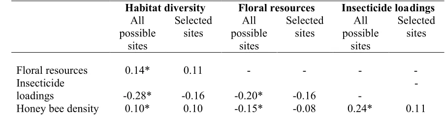
In terms of the correlations between validated metrics, there were significant relationships 294
between the metrics for three out of the six pair wise comparisons overall (Table 4), although 295
the correlation coefficients were all below the commonly used threshold of 0.7 for including 296
variables in the same analysis. Measured floral resources was significantly correlated with 297
measured honey bee density (Spearman’s ρ = 0.31, p = 0.002) and with measured insecticide 298
loadings (Spearman’s ρ = 0.47, p <0.05). In addition, measured honey bee density was 299
strongly linked to measured insecticide loadings (Spearman’s ρ = 0.54, p <0.05). However, 300
for the individual regions (Fig. S7 – S9) the only significant correlations were for measured 301
habitat diversity vs measured honey bee density in Inverness (Spearman’s ρ = 0.54, p =0.03; 302
Fig. S7), measured insecticide loadings vs measured habitat diversity in Wiltshire 303
(Spearman’s ρ = 0.92, p <0.01; Fig S9) and for measured honey bee density vs measured 304
insecticide loadings in Cambridgeshire (Spearman’s ρ = 0.65, p = 0.04; Fig. S9). 305
15 $
307
The methodology described here aimed to build on previous site selection protocols to select 308
sites that varied in four main gradients, while at the same time ensuring comparability 309
between sites and representation of Britain more widely. Although estimations of the four 310
metrics were made with some uncertainty, the low level of correlation between verified 311
metrics at the regional and national scales suggest that the site selection method provides a 312
suitable sample of sites for investigating links between land management and pollinator 313
biodiversity. 314
315
316
One of the main differences between previous approaches and our protocol is in the objective 317
selection of study regions, chosen here to represent Britain in terms of land class and land 318
cover variables. Regions are often chosen in landscape studies because they are well known 319
and have been used several times before in previous work. This manner of selecting focal 320
regions is sufficient for studies that aim to understand basic or local mechanisms or 321
processes. For example, Watts . (2016) chose two regions of the UK due to previous 322
knowledge of the areas and of the variation in woodland habitats. Such a selection approach 323
was expedient and suitable for the authors’ study question which focused on landscape 324
conservation and links between woodland biodiversity and gradients of woodland 325
characteristics. Furthermore, the inferential scope of this study is likely restricted to British 326
lowland woodlands within these two regions. By contrast, our research project sought to link 327
the regional variation in land management drivers across a broad range of habitat types to the 328
regional variation in pollinator diversity, thereby supporting inference about Britain as a 329
16 be more objectively selected (Dilts, Yang & Weisberg 2010) and subject to the same levels of 331
control as site selection. The addition of this regional selection protocol is therefore 332
recommended for studies seeking broad statistical inference and a replicated pseudo 333
experimental design (Table 1). 334
335
336
The second main difference in our approach was in the number of focal variables used 337
simultaneously to select sites. Previous approaches have selected sites for different variables 338
in a similarly hierarchical fashion, simultaneously selecting sites based on two variables 339
(Holzschuh, Steffan Dewenter & Tscharntke 2010; Hopfenmueller, Steffan Dewenter & 340
Holzschuh 2014; Steckel 2014). Some such studies also detail selecting sites in the four 341
quadrants of a 2 dimensional bivariate plot to remove the correlation between variables in the 342
selected sites (Fahrig . 2011; Pasher ., 2013). Pasher . (2013) further suggested 343
the extension of this selection system to dimensions, and Watts . (2016) attempted it 344
with three dimensions. However, each additional selection variable greatly increases the 345
number of possible combinatorial possibilities, which can soon become unmanageable. Here, 346
we have presented the first attempt to use four dimensions and provide detailed instructions 347
for manageable repetition of the method. 348
While there was some uncertainty in estimating our four metrics, the set of sites selected was 349
sufficiently dispersed in variable space to allow analysis using continuous variables with 350
values across the full ranges of each (Pasher . 2013). Randomly selected focal sites tend 351
to cluster around mean values, providing relatively low resolving power for discerning the 352
effects of landscape scale drivers. Our original choice of what were modelled to be extreme 353
17 imprecise models combined with the inevitable regression towards the mean resulted in a 355
wide exploration of parameter space of variables individually and in combination. An 356
additional benefit of the protocol is that it greatly reduces the degree of correlation between 357
focal variables, allowing valid inferences to be drawn about their separate and interacting 358
impacts (Eigenbord . 2011; Pasher . 2013). Furthermore, studies of this kind do not 359
normally assess correlations based on validated data, but we have demonstrated here that 360
some caution is required if the calculation of focal variables is subject to high levels of 361
uncertainty. Improvements to our metric estimates are likely to lead to further decoupling of 362
metrics at the national scale. 363
364
365
The estimates of the four metrics varied in their accuracy quite widely. The most accurate 366
was the habitat diversity metric which was based on the proportion of habitat covers 367
calculated from remote sensing data. The high accuracy of this metric is not surprising as the 368
estimates required the fewest steps in making the calculations, and verification was relatively 369
straightforward. Even where the precise nature of land cover was misclassified on LCM2007, 370
the spatial configuration of habitats as determined on the ground, and thus the Shannon index 371
value, was generally quite close to our estimates from the LCM data. The level of accuracy is 372
also similar to previous verification efforts (Morton 2011). 373
The insecticide metric was also relatively well predicted when only considering those fields 374
for which questionnaire responses were received. However, this result masks the large 375
number of tetrads (especially in the North) for which large positive insecticide loadings were 376
predicted when no arable fields were found on the ground. Although insecticides are applied 377
18 loading value. These inappropriate values were probably caused in part by the satellite
379
classification of reseeded pastures as arable fields and partly by changes in the crop areas 380
between the 2010 census and 2012/13 survey years due to normal crop rotation. 381
The floral resource metric proved to have relatively low accuracy for a number of reasons 382
related to the data available for making estimates: 1) some habitat cover estimates were 383
incorrect due to misclassification in LCM2007 as described above, 2) actual floral reward 384
data were only available for relatively few species at the time of site selection, 3) estimates of 385
species cover per habitat were based on regional averages per broad habitat and so were not 386
sensitive to within region variation, and 4) mean nectar availability reported in databases 387
does not capture the high variability observed in the field due to site differences in climate, 388
soil and nectar consumption. Validation of these factors inevitably led to some widely 389
differing values of site level floral resource availability. 390
The honey bee density metric was the least well verified of the four drivers partly because the 391
methods used to count the number of honey bees visiting sites proved to be unsuitable. As 392
honey bees are social foragers, using scouts to alert workers to rich floral resource patches, 393
the use of pan trapping to sample them is extremely inefficient (Westphal 2008). 394
Further, attempts to observe honey bees on the wing or foraging along transects suffered from 395
a lack of available survey time: only 3 full days per season per site were used, often in poor 396
weather conditions. Where data are available, they show a good relationship with the 397
estimated density. However, such is the noise in the data and the high presence of zeros that 398
subsequent analysis will need to use the original estimated values as an explanatory variable. 399
Better estimates of honey bee numbers would require either greater investment in survey time 400
or an alternative method such as the use of baited traps or estimating the number of hives 401
19 problems, we are not able to verify the accuracy of the honey bee population density
403
estimation technique. 404
405
406
The aims of this site selection methodology were to improve on previous landscape scale 407
natural experimental designs by i) increasing objectivity of region selection to enhance the 408
ability to generalise results to the wider landscape, and ii) to improve the selection of sites 409
based on the values of multiple focal variables. This has been achieved by developing a 410
hierarchical region selection protocol and by explicitly testing previously conceived ideas of 411
site selection using multiple variables simultaneously. The additional complexities we have 412
introduced to landscape scale site selection will not be necessary for every research question, 413
but provide a basis for increasing the inferential scope and complexity of landscape scale 414
pseudo experiments. 415
We have also shown that it is possible to use national datasets to derive credible and objective 416
sets of study sites that cover multiple environmental gradients, without bias from researcher’s 417
personal knowledge of landscapes in the site selection. The implications of this 418
methodological development are important for landscape ecology and national scale 419
monitoring programmes in any region or country with sufficient data, with a network of well 420
chosen sampling sites being a vital tenet of a well designed national monitoring scheme. 421
422
% &
423
We are especially grateful to our network of farmers, landowners and land managers who 424
20 conducting the field work: Nicole Dunn, Hayley Wiswell, Ewan Munro, Katy Donald, Jessica 426
Heikkinen, Katherine White, Clare Pemberton, Paul Webb, Mark Tilzey, Sara Iversen, Robin 427
Curtis, Paul Hill, Sam Bacon, Paul Wilson, Bex Cartwright, John Fitzgerald, Patrick 428
Hancock, Mel Stone, Robert Day, James McGill, Tracie Evans. Kate Somerwill and Mette 429
Kusk Gillespie are thanked for assistance with the protocol design. This research was 430
supported by the UK Insect Pollinator Initiative project “AgriLand: Linking agriculture and 431
land use change to pollinator populations”, funded under the Living with Environmental 432
change programme, a collaboration between Biotechnology and Biological Sciences 433
Research Council (BBSRC), the Wellcome Trust, Scottish Government, Department of 434
Environment, Food and Rural Affairs (DEFRA) and Natural Environment Research Council 435
(NERC): grant BB/H014934/1 (www.agriland.leeds.ac.uk). 436
437
$ All primary collected datasets (datasets collected during the course of the 438
project), are stored in the Centre for Ecology & Hydrology data repository and will be made 439
available for download following publication of this manuscript. Other datasets used as cited 440
in the article are available to download from the sources cited. 441
442
443
Baude, M., Kunin, W.E., Boatman, N.D., Conyers, S., Davies, N., Gillespie, M.A.K., 444
Morton, R.D., Smart, S.M. & Memmott, J. (2016) Historical nectar assessment 445
reveals the fall and rise of floral resources in Britain. '()* 85 88. 446
Beekman, M. & Ratnieks, F.L.W. (2000) Long range foraging by the honey bee, Apis 447
21 Brittain, C.A., Vighi, M., Bommarco, R., Settele, J. & Potts, S.G. (2010) Impacts of a
449
pesticide on pollinator species richness at different spatial scales. 450
!!* 106 115. 451
Bunce, R.G.H., Barr, C.J., Clarke, R.T., Howard, D.C. & Lane, A.M.J. (1996) ITE 452
Merlewood Land Classification of Great Britain. ! " ,(* 625 453
634. 454
Carey, P.D., Wallis, S., Chamberlain, P.M., Cooper, A., Emmett, B.A., Maskell, L.C., 455
McCann, T., Murphy, J., Norton, L.R., Reynolds, B., Scott, W.A., Simpson, I.C., 456
Smart, S.M. & Ullyett, J.M. (2008) Countryside Survey: UK Results from 2007. 457
Centre for Ecology & Hydrology. 458
Diamond, J.M. (1983) Ecology laboratory, field and natural experiments. ()+* 586 459
587. 460
Dilts, T.E., Yang, J. & Weisberg, P.J. (2010) The Landscape Similarity Toolbox: new tools 461
for optimizing the location of control sites in experimental studies. ((* 462
1097 1101. 463
Eigenbrod, F., Hecnar, S.J. & Fahrig, L. (2011) Sub optimal study design has major impacts 464
on landscape scale inference. Biological Conservation, 144, 298 305. 465
Elbgami, T., Kunin, W.E., Hughes, W.O.H. & Biesmeijer, J.C. (2014) The effect of 466
proximity to a honeybee apiary on bumblebee colony fitness, development, and 467
performance. +'* 504 513. 468
Evison, S.E.F., Roberts, K.E., Laurenson, L., Pietravalle, S., Hui, J., Biesmeijer, J.C., Smith, 469
J.E., Budge, G. & Hughes, W.O.H. (2012) Pervasiveness of Parasites in Pollinators. 470
# -.
22 Fischer, C., Thies, C. & Tscharntke, T. (2011) Mixed effects of landscape complexity and 472
farming practice on weed seed removal. Perspectives in Plant Ecology Evolution and 473
Systematics, 13, 297 303. 474
Gabriel, D. & Tscharntke, T. (2007) Insect pollinated plants benefit from organic farming. 475
$ !!.* 43 48.
476
Gabriel, D., Sait, S.M., Hodgson, J.A., Schmutz, U., Kunin, W.E. & Benton, T.G. (2010) 477
Scale matters: the impact of organic farming on biodiversity at different spatial scales. 478
Ecology Letters, 13, 858 869. 479
Goulson, D. & Sparrow, K. (2009) Evidence for competition between honeybees and 480
bumblebees; effects on bumblebee worker size. ! " % & !(* 481
177 181. 482
Hargrove, W.W. & Pickering, J. (1992) Pseudoreplication a sine qua non for regional 483
ecology. ' /* 251 258. 484
HilleRisLambers, J., Ettinger, A.K., Ford, K.R., Haak, D.C., Horwith, M., Miner, B.E., 485
Rogers, H.S., Sheldon, K.S., Tewksbury, J.J., Waters, S.M. & Yang, S. (2013) 486
Accidental experiments: ecological and evolutionary insights and opportunities 487
derived from global change. ( !,,* 1649 1661. 488
Holzschuh, A., Steffan Dewenter, I. & Tscharntke, T. (2010) How do landscape composition 489
and configuration, organic farming and fallow strips affect the diversity of bees, 490
wasps and their parasitoids? ! " -0* 491 500. 491
Hopfenmueller, S., Steffan Dewenter, I. & Holzschuh, A. (2014) Trait Specific Responses of 492
Wild Bee Communities to Landscape Composition, Configuration and Local Factors. 493
# 0.
23 Morton, D., Rowland, C., Wood, C., Meek, L., Marston, C., Smith, G., Wadsworth, R. & 495
Simpson, I. (2011) Final Report for LCM2007 the new UK land cover map. 496
& . Centre for Ecology & Hydrology.
497
Pasher, J., Mitchell, S.W., King, D.J., Fahrig, L., Smith, A.C. & Lindsay, K.E. (2013) 498
Optimizing landscape selection for estimating relative effects of landscape variables 499
on ecological responses. Landscape Ecology, 28, 371 383. 500
Potts, S.G., Vulliamy, B., Dafni, A., Ne'eman, G. & Willmer, P. (2003) Linking bees and 501
flowers: How do floral communities structure pollinator communities? .+* 502
2628 2642. 503
R Core Team (2014) R: A Language and Environment for Statistical Computing. R 504
Foundation for Statistical Computing, Vienna, Austria. 505
Rortais, A., Arnold, G., Halm, M.P. & Touffet Briens, F. (2005) Modes of honeybees 506
exposure to systemic insecticides: estimated amounts of contaminated pollen and 507
nectar consumed by different categories of bees. (/* 71 83. 508
Rundlof, M., Andersson, G.K.S., Bommarco, R., Fries, I., Hederstrom, V., Herbertsson, L., 509
Jonsson, O., Klatt, B.K., Pedersen, T.R., Yourstone, J. & Smith, H.G. (2015) Seed 510
coating with a neonicotinoid insecticide negatively affects wild bees. ',!* 77 511
U162. 512
Sagarin, R. & Pauchard, A. (2010) Observational approaches in ecology open new ground in 513
a changing world. .* 379 386.
514
Shackelford, G., Steward, P.R., Benton, T.G., Kunin, W.E., Potts, S.G., Biesmeijer, J.C. & 515
Sait, S.M. (2013) Comparison of pollinators and natural enemies: a meta analysis of 516
landscape and local effects on abundance and richness in crops. )
517
24 Smart, S.M., Henrys, P.A., Purse, B.V., Murphy, J.M., Bailey, M.J. & Marrs, R.H. (2012) 519
Clarity or confusion? Problems in attributing large scale ecological changes to 520
anthropogenic drivers. % ,)* 51 56. 521
Smart, S.M., Ellison, A.M., Bunce, R.G.H, Marrs, R.H., Kirby, K.J., Kimberley, A., Scott, 522
W.A. & Foster, D.R. (2014) Quantifying the impact of an extreme climate event on 523
species diversity in fragmented temperate forests: the effect of the October 1987 524
storms on British broadleaved woodlands. Journal of Ecology, 102, 1273 1287. 525
Steckel, J., Westphal, C., Peters, M.K., Bellach, M., Rothenwoehrer, C., Erasmi, S., Scherber, 526
C., Tscharntke, T. & Steffan Dewenter, I. (2014) Landscape composition and 527
configuration differently affect trap nesting bees, wasps and their antagonists. 528
& !-,* 56 64.
529
Waddington, K.D., Visscher, P.K., Herbert, T.J. & Richter, M.R. (1994) Comparisons of 530
forager distributions from matched honey bee colonies in suburban environments. 531
* ('* 423 429. 532
Watts, K., Fuentes Montemayor, E., Macgregor, N.A., Peredo Alvarez, V., Ferryman, M., 533
Bellamy, C., Brown, N. & Park, K.J. (2016) Using historical woodland creation to 534
construct a long term, large scale natural experiment: the WrEN project. Ecology and 535
Evolution, 6, 3012 3025 536
Westphal, C., Bommarco, R., Carre, G., Lamborn, E., Morison, N., Petanidou, T., Potts, S.G., 537
Roberts, S.P.M., Szentgyorgyi, H., Tscheulin, T., Vaissiere, B.E., Woyciechowski, 538
M., Biesmeijer, J.C., Kunin, W.E., Settele, J. & Steffan Dewenter, I. (2008) 539
Measuring bee diversity in different european habitats and biogeographical regions. 540
25 Westphal, C., Steffan Dewenter, I. & Tscharntke, T. (2006) Bumblebees experience
542
landscapes at different spatial scales: possible implications for coexistence. 543
!+0* 289 300. 544
Zuur, A.F., Ieno, E.N., Walker, N.J., Saveliev, A.A., & Smith, G.M. (2009) Mixed Effects 545
Models and Extensions in Ecology with R. Springer, New York. 546
26 548
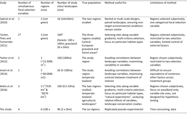
Table 1: Comparison of previous and current site selection protocols of studies incorporating a landscape scale pseudo experimental approach 549
Study Number of simultaenous focal selection variables Number of regions (size)
Number of study sites/ landscapes (size)
True population Method useful for: Limitations of method
Gabriel et al.
(2010)
1 2 (not
given)
16 (10x10km) The two regions studied
Nested or multi-scale designs, paired landscapes, ensuring non-target environmental conditions remain similar
Regions selected subjectively, one categorical focal selection variable
Fischer, Thies and Tscharntke (2011)
2* 3 (not
given)
100*
(forests: 100 x 100m; grassland: 50 x 50m)
The three regions studied; Central European grassland and forest areas?
Selecting sites along variable gradients, multi-criteria selection, focus on particular habitat types
Regions selected subjectively, restricted to two selection variables, limited control of external factors
Pasher et al.
(2013)
2 1
(~15,500k m2 )
100 (100ha) The study region
Avoiding correlations between landscape variables, maximizing variability in variables
Region chosen subjectively, restricted to two selection variables
Smart et al. (2014)
1 2
(~60,000k m2)
26 (5-100ha) The study region; temperate lowland
Avoiding correlations between landscape variables, maximizing contrast between treatment of interest
Difficult to ensure equivalence of numerous other factors across treatment groups
Watts et al.
(2016)
3 2 (~7335
km2 & ~8570 km2)
106 (0.5-32ha) The two regions studied; temperate lowland agricultural landscapes?
Selecting sites along variable gradients, multi-criteria selection, focus on particular habitat types, “natural experiments”, analyzing relative effects of variables, landscape conservation studies
Regions chosen subjectively, focus on woodland only, variable site sizes, not designed for hypothesis testing
27
100km) the British
countryside
designs, broad generality of results, hypothesis testing
intensive
28 Table 2: Spearman correlation coefficients for the four & metrics (i.e., before
551
ground truthing; Box Cox transformed Z scores) for all six study regions. Coefficients are 552
calculated for all possible sites within all regions (n = 12,718 sites) and the sites selected for 553
study (n = 96). Asterisks denote significant correlations (p<0.001). Partial correlation 554
coefficients were calculated controlling for Region, but are not shown as they were not 555
different from the coefficients below. 556
All possible
sites
Selected sites
All possible
sites
Selected sites
All possible
sites
Selected sites
Floral resources 0.14* 0.11 Insecticide
loadings 0.28* 0.16 0.20* 0.16
Honey bee density 0.10* 0.10 0.15* 0.08 0.24* 0.11
29 Table 3: Spearman’s rank correlation and partial correlation coefficients (controlling for 558
Region), and parameters of linear mixed models (Region as random effect) for the estimated 559
versus measured metrics in all regions. The data are Z scores: box cox transformed and zero 560
centred. “Mean floral resources” is the total amount of floral resources averaged over the two 561
years of field sampling. Asterisks indicate significant correlations: *** = p<0.001, ** = 562
p<0.01, * = p<0.05 563
1 2 3 2
Habitat diversity 0.77*** 0.77*** 0.56 0.05 <0.001 Mean floral resources 0.28** 0.29** 0.20 0.03 0.005 Insecticide loadings 0.67** 0.60** 0.67 0.01 0.001
Honey bee density 0.22* 0.21* 0.16 0.03 0.002
564
30 Table 4: Spearman’s rank correlation and partial correlation (controlling for region)
566
coefficients for the four & metrics (i.e., corrected metrics after ground truthing; Box 567
Cox transformed Z scores) for all six study regions. Asterisks indicate significant correlations 568
(* = p<0.05, ** = p<0.01). 569
Floral resources 0.18
Insecticide loadings 0.47* 0.10
Honey bee density 0.04 0.31** 0.54*
,
-Floral resources 0.16
Insecticide loadings NA NA
Honey bee density 0.05 0.29** NA
570
571
31 573
574
Fig. 1: The extent of the six 100 km2 regions chosen by the region selection protocol (blue 575
squares), and the 96 field sites (sixteen 2 x 2 km2 sites per region) chosen by the site selection 576
protocol (red circles). (Service Layer Credit: OS data; Crown copyright and database right 577
2015) 578
579
Fig. 2: The estimated Z scores (Box Cox transformed and zero centred data) of the four 580
metrics for the final 16 sites of the Cambridgeshire/Suffolk region, shown here as an 581
example. The blue bars are Z scores above 0, i.e., the site has a “high” score for that metric; 582
the red bars are negative Z scores, i.e., the site has a “low” score for that metric. The 16 sites 583
represent every combination of high and low values of the four metrics, e.g., site 1 has high 584
values of all four metrics, site 2 has a low value only for habitat diversity, and so on. The data 585
for the remaining regions can be found in Fig. S3. 586
587
Fig. 3: “Ground truthing” of the four key metrics. The data are Z scores: box cox 588
transformed and 0 centred, and each point represents a single site. The straight bold line 589
represents the linear regression line for all regions and the shaded area represents 95% 590
confidence intervals. The blue lines are mixed effect regression lines for each of the six 591
regions with “region” as a random effect, displayed here to demonstrate the variation in 592
prediction accuracy between regions. “Mean floral resources” is the total amount of floral 593
resources averaged over the two years of field sampling. Regional graphs are shown in Fig. 594
For Review Only
! " #
$ % & '" ( % ) *
+ !
! " # $ % &!
$ $! ' ( ) % ! $ $! ' "(
$ # % * " % !
$ $! % ! + " % * % *! $
, $ -$
, $ +
! "
# $ % "
# $& %
" " # ' # ( )*
( +