Chapter 6: Ice-Phase Precipitation

Chapter 6

Ice-Phase Precipitation

I. GULTEPE

Cloud Physics and Severe Weather Research Section, Environment Canada, Toronto, Ontario, Canada

A. J. HEYMSFIELD

National Center for Atmospheric Research, Boulder, Colorado

P. R. FIELD

Met Office, Exeter, and School of Earth and Environment, Institute for Climate and Atmospheric Science, University of Leeds, Leeds, United Kingdom

D. AXISA

National Center for Atmospheric Research, Boulder, Colorado

ABSTRACT

Ice-phase precipitation occurs at Earth’s surface and may include various types of pristine crystals, rimed crystals, freezing droplets, secondary crystals, aggregates, graupel, hail, or combinations of any of these. Formation of ice-phase precipitation is directly related to environmental and cloud meteorological param-eters that include available moisture, temperature, and three-dimensional wind speed and turbulence, as well as processes related to nucleation, cooling rate, and microphysics. Cloud microphysical parameters in the numerical models are resolved based on various processes such as nucleation, mixing, collision and co-alescence, accretion, riming, secondary ice particle generation, turbulence, and cooling processes. These processes are usually parameterized based on assumed particle size distributions and ice crystal microphysical parameters such as mass, size, and number and mass density. Microphysical algorithms in the numerical models are developed based on their need for applications. Observations of ice-phase precipitation are performed using in situ and remote sensing platforms, including radars and satellite-based systems. Because of the low density of snow particles with small ice water content, their measurements and predictions at the surface can include large uncertainties. Wind and turbulence affecting collection efficiency of the sensors, calibration issues, and sensitivity of ground-based in situ observations of snow are important challenges to assessing the snow precipitation. This chapter’s goals are to provide an overview for accurately measuring and predicting ice-phase precipitation. The processes within and below cloud that affect falling snow, as well as the known sources of error that affect understanding and prediction of these processes, are discussed.

1. Introduction

The major components of snow precipitation are re-lated to processes occurring in and below clouds such as nucleation, depositional growth, collision–coalescence, accretion, aggregation, sublimation, secondary ice gen-eration, and freezing. Thermodynamical and dynamical conditions affect the rate at which these processes occur,

and hence both the intensity and amount of snow within the cloud and at the surface. Thus, for accurate pre-diction of snow, knowledge of not only microphysical processes within the cloud but also conditions related to the ambient dynamics and thermodynamics of the sys-tem are required.

The goals of this chapter are to provide an overview of what is important for accurately observing and predict-ing ice-phase precipitation, the processes within and below cloud that affect falling snow, the known sources Corresponding author: Ismail Gultepe, [email protected]

DOI: 10.1175/AMSMONOGRAPHS-D-16-0013.1

of error that affect the understanding and prediction of these processes, and the steps needed to improve snow estimates. Prediction of solid precipitation based on various model types that include cloud, numerical weather prediction (NWP), and climate models can in-clude issues related to scale and downscaling issues, microphysical schemes, parameterizations, data assimi-lation, and boundary conditions. Thus, specific sections on methods used to measure snow, its prediction, and their inherent limitations and uncertainties, are pre-sented. The current status of the prediction of snow precipitation at various scales and the effects of snow on weather, climate, and society are included, as well as recommendations for future work.

2. Description of the ice-phase precipitation and microphysics

Solid precipitation, including both single and complex snow crystals, is very important in precipitation process. Based on the American Meteorological Society (AMS) Glossary of Meteorology (American Meteorological Society 2016a), snow is defined as precipitation com-posed of white and/or translucent ice crystals, chiefly in complex branched hexagonal form and often aggregated into snowflakes that fall onto Earth’s surface. Ice crystal formation can occur because of various nucleation processes. These nucleation processes (seeKanji et al. 2017, chapter 1) are usually defined as 1) homogeneous nucleation and 2) heterogeneous nucleation (Gultepe et al. 2016). Depending on ice nuclei chemical and physical properties, ice crystals as a function of dynam-ical and thermodynamic conditions can have various habit and particle size distributions. After nucleation, ice crystals of different habits such as ‘‘pristine’’ needles, plates, columns, dendrites, and stellar crystals grow ac-cording to the relative humidity RH with respect to water (RHw) and temperature T. However, observed

particles commonly have many nonpristine shapes. Lawson et al. (2006) reported that irregularly shaped ice crystals atTbetween2308and2408C were observed in an Antarctic site during all types of falling ice crystal precipitation and in blowing snow, which was prevalent when the wind speed was 4 m s21. Irregular ice crystals in blowing snow were observed to generally have more rounded edges than irregular shapes in precipitation. These were consistent with diamond dust, and falling ice fog/light snow particles were observed in the Arctic re-gion (Gultepe et al. 2015). In addition to diffusional growth, collision and aggregation because of turbulence, eddies, and different fall velocities, as well as collection and freezing of supercooled droplets (riming), can affect precipitation characteristics. Under mixed-phase and

dynamically active conditions, ice particles can develop into graupel and hail at higher altitudes in the cloud. The terminal velocityVtof ice crystals is typically between

0.1 and 3 m s21, and the vertical air velocitywaplays an

important role in the particle growth and ultimately snow precipitation intensity (Heymsfield et al. 2007;

Gultepe et al. 1995; Gultepe and Starr 1995). Snow crystal densities (mass divided by spherical volume based on particle maximum size) usually vary from 0.05 to 0.20 g cm23, which is size dependent because mass is related to crystal size (Cotton et al. 2013). After pre-cipitating ice particles fall below cloud base, they ex-perience evaporation, turbulence, collision and mixing processes before reaching the ground. A large frac-tion of Earth’s rain originates as snow that subse-quently melts before reaching the ground (Field and Heymsfield 2015).

The increasing size of ice particles depends on both the dynamics of the system (e.g., turbulence, eddies, updrafts) and the thermodynamics of the environment (e.g., cooling rates and ice nuclei) (Gultepe et al. 2000). Further growth of ice particles by riming and aggrega-tion is a funcaggrega-tion of the droplet spectra and ice crystal morphology, which affects the ice particle–droplet or ice crystal–crystal collision efficiency (defined as the ratio of collisions to all particles) and the aggregation efficiency (defined as ratio of merging ice crystals to all collisions (Pflaum and Pruppacher 1979). Mixed-phase conditions leading to snow can also be affected by ice crystals at the expense of droplets, which is a result of the vapor pressure difference between droplet and ice particle surfaces (Bergeron 1935) and through the riming process.

Ice microphysical properties can be related to ice nuclei (IN) physical properties and their chemical composition (Shantz et al. 2014). The IN number con-centration plays an important role for ice crystal growth that is a function of both T and available moisture. Previous studies suggest ice crystal number concentra-tions Ni within a cloud may well exceed those of ice

nucleating particles (INPs) based on observations and parameterizations (e.g., Fletcher 1962; Hobbs 1975). These studies suggested that ice multiplication may have occurred when the measured Ni is much larger than

predicted by theFletcher (1962)study for a given tem-perature. Ice multiplication here is defined as increasing Ni based on microphysical, dynamical, and

glaciation of a cloud (Lawson et al. 2015), leading to increasing precipitation.

The aggregation (combination of two or more crys-tals) of ice crystals plays an important role for snow precipitation intensity because of increasing mass (Lo and Passarelli 1982). It depends on the relative terminal velocity of the aggregated components, their sticking efficiency (defined as possibility of joining together of particles after the collision;Phillips et al. 2015), wind shear, turbulence, T, RH, and electrical charge (Saunders and Wahab 1975). The density and shape of the ice particles, which influences the precipitation amount (PA) and snow depth, are strong functions of the environmental conditions that affect the ice nucle-ation processes, radiative heating, cooling, and turbu-lence. More specifically, the rate of collision depends upon the relative fall speeds and sizes (Stokes num-ber), cross-sectional areas and, possibly, electrical charge. The nature of crystal attachment in the at-mosphere is not well understood, but potentially im-portant factors for controlling the sticking efficiency are related to the shape of ice crystals (e.g., mechan-ical interlocking of dendrites), surface properties (also its morphology;Phillips et al. 2015), and atmo-spheric thermodynamical properties (T, RH) that promote rapid sintering between crystals and electrical charges. Laboratory investigations into aggregation of snow particles were studied by Hosler and Hallgren (1960)andConnolly et al. (2012). On the other hand, a few aircraft-based attempts at quantifying sticking efficiency were also performed by Passarelli (1978),

Mitchell (1988),Field and Heymsfield (2003), andField et al. (2006). These studies typically show that 1 collision in 10 results in a sticking event if a simple gravitational collection kernel is used to estimate the rate at which collisions occur.

Below the cloud base, subsaturation of air with re-spect to ice can result in sublimation of the ice and snow particles. When air becomes slightly less saturated with respect to water below the cloud base, then ice particle growth during fall can still occur (Field et al. 2007;

McFarquhar et al. 2007). This growth can affect the snow water equivalent (SWE, defined as the ratio of melted snow amount to snow depth) of the precipitation on the ground and needs to be studied because aggre-gation during sublimation is usually neglected in mod-eling simulations.

In clouds with strong updrafts, riming of snow crystals, snowflakes, and graupel particles may con-tinue where hail can develop (Knight et al. 1982). Hail, by definition, has a diameter of 5 mm or more (Lin et al. 1983). The AMS Glossary of Meteorology (American Meteorological Society 2016b) defines

graupel as heavily rimed snow particles that are dis-tinguished by conical, hexagonal and lump forms, whereas hail is defined as balls or irregular lumps of ice (American Meteorological Society 2016b,c). The bulk density of these particles is related to the ice particle surface, environmentalTand RH, and the liquid water content. The bulk microphysics algorithms in cloud or forecast models, with varying degrees of com-plexity (one- or two-moment schemes), can be used to predict parameters related to cloud ice crys-tals, precipitating snow particles, graupel, and hail (Morrison and Milbrandt 2011). Microphysical pro-cesses for converting between hydrometeor types are not well constrained.Figure 6-1(fromTomita 2008)

shows the major components of a six-class micro-physical scheme used in simulations of cloud systems. The major components of this scheme are vapor, cloud water, cloud ice, rain, and snow, as well as graupel. Interactions among these components are shown with various transformations. The rate at which these transformations occur is highly dependent on as-sumptions used in the scheme, including the spectral form of size distributions and particle fall velocities, shapes, and collection efficiencies. A major un-certainty for snow formation is to better understand how the autoconversion process is parameterized be-tween various phases of snow and ice crystals, and develop physically based particle growth models without preassumed empirical relationships for mi-crophysical parameters.

In this chapter, snow measurements and microphysics are provided in section 3. The cloud microphysics are given insection 4. Then snow prediction issues based on various numerical models are summarized. Section 6

focuses on precipitation efficiency calculation and re-lated issues. Snow precipitation’s effects on weather, climate, and society are analyzed insection 7.Sections 8

and9summarize the challenges to understanding snow precipitation and recommendations for future work, respectively.

3. Snow measurements and microphysics

sensors; Table 6-1] also provide PA and PR, and bulk precipitation type. SWE is usually obtained by a ratio of measuring melted amount of snow (mm) measured by weighing gauges to snow depth (mm) measured by snow rulers or snow depth sensors such as SR50, and it can change from a few percent up to more than 50% de-pending on snow particle morphology.

By definition, snow precipitation can include various particle shapes and types, and the SWE ratio is usually assumed to be 10% by forecasters. The U.S. National Weather Service (NWS) previously used a SWE con-version table as a function ofT(Table 6-2;NWS 1996;

Dubé2003). It is unlikely that this table will be used operationally because of the variability in SWE as a function of temperature and particle type. The amount of water within the snow can play an important role for the hydrological cycle, environmental processes, and also for transportation and aviation. The surface

skin temperatures can also affect precipitation type, for example, freezing drizzle, rain, or snow. Snow types can also be divided into various subgroups such as ice or snow pellets, wet snow and ice crystals (Dubé 2003). Figure 6-2 shows various snow particle types collected during the Fog and Remote Sensing and Modeling (FRAM) and Satellite Application for Arctic Weather and Search and Rescue (SAR) Operations (SAAWSO) projects (Gultepe et al. 2015; Rabin et al. 2016).

Ice pellets (or sleet) are usually defined as frozen raindrops (Dubé 2003). Based on their density, ice pellets can be classified into the heavy snow category. He stated that in the presence of a deep warm layer (T . 38C) above a layer with freezing temperatures (T, 258C), drops can form from melting of the snow crystals in the warm layer, then fall into the cold air layer, leading to their freezing and formation of sleet.

Snow grains (frozen water droplets) are also included in this category. Details on the basic precipitation processes for modeling applications have been de-scribed in many studies, including Lin et al. (1983),

Tomita (2008), Ferrier (1994), Ferrier et al. (1995),

Milbrandt and Yau (2005), andMorrison et al. (2005). In the following sections, snow measurements and its microphysics are provided.

a. Weighing gauge measurements and uncertainties

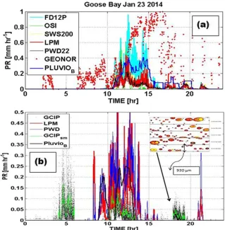
Weighing precipitation gauges are affected by the environmental conditions, especially by the horizon-tal wind speeds and turbulence. Under relatively calm wind conditions (horizontal wind speedUh,5 m s21),

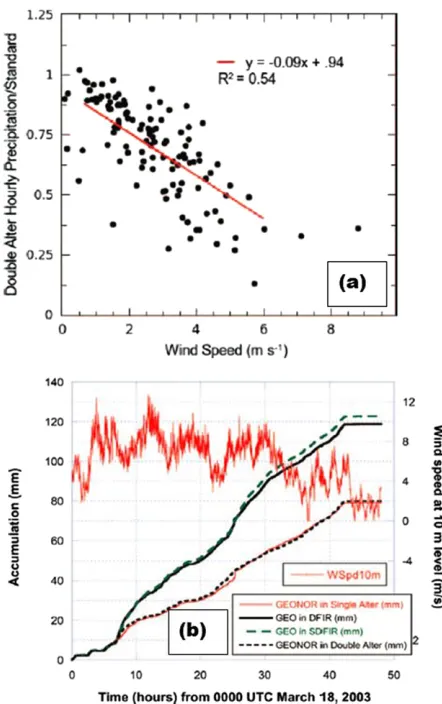
Geonor and Pluvio (Fig. 6-3a) measurements may not need wind corrections for heavy rain but their sensi-tivity for light snow (LSN) and light rain (LRN), in-cluding drizzle, can be an important issue (Gultepe et al. 2016; Leeper et al. 2015). Usually, a double-fenced weighing gauge (Fig. 6-3b) is used for refer-ence snow measurements.Figure 6-3cshows the en-tire project area called PanAm University of Ontario Meteorological Supersite (PUMS) nearby Oshawa, Ontario, Canada. Both Pluvio and Geonor measure-ments with an alter shield in a bush environment or within a double-fenced international reference (DFIR) system are usually accepted as reference for precipitation measurements. Geonor observations of snow PR have an uncertainty of 0.1 mm h21based on the factory specification, but this sensitivity can be up to 0.5 mm h21 with turbulence and stronger wind conditions (Gultepe et al. 2016). The Geonor weigh-ing gauge utilizes a technology based on three vi-brating wires to measure the weight of melted snow

in a bucket to distribute the snow mass equally. These measurements are then converted to precipitation amount over 5–10-min intervals. Another sensor for the snow measurements can be used is the total pre-cipitation sensor (TPS; Rasmussen et al. 2012). Al-though its measurements can be reliable for stable atmospheric conditions, because of high winds and strong turbulence, TPS measurements can include large uncertainties (Boudala et al. 2014). For winds greater than 8 m s21, a 1 mm h21 threshold value is needed to obtain accurate PR for both the TPS and Geonor 5-min averaged measurements (Rasmussen et al. 2012).

b. Optical probes

As stated above, snow measurements at the surface can be measured by optical probes based on the ex-tinction coefficient and spectral snow crystal charac-teristics. The Ground Cloud Imaging Probe (GCIP;

Fig. 6-4a) was developed by Environment Canada (Fig. 6-4a). It is based on the Droplet Measurement Technologies (DMT) Cloud Imaging Probe (CIP), which

TABLE6-1. Shows precipitation- and visibility-measuring sensors (Gultepe et al. 2016). Precipitation type (PT), precipitation rate (PR), particle spectra (PS) and amount (PA), visibility (Vis), fall velocity (Vf), and diameter (D).

Precipitation and Vis sensors

Manufacturing

company Measurements Threshold PR, PA, Vis

GCIP DMT PS, shape 0.01 mm h21

PWD22 Vaisala PT, PR, PA, Vis 0.01 mm min21_{(0.05 mm h}21_{), 0.01 mm and 10%,}

.2408C, 10 m (10%)

FD12P Vaisala PT, PR, PA, Vis 0.02 mm min21_{(0.05 mm h}21_{), 0.01 mm and 10%,}

.2408C, 10 m (10%)

SWS200 Biral PT, PR, PA, Vis 0.0015 mm h21_{, 0.001 mm, 10 m, 5%,.2408C}

OSI-430 Optical Scientific PT, PR, PA, Vis 0.01 mm h21_{, 0.001 mm, 0.001 km,.2408C}

Sentry Envirotech Vis 10%, 30 m,.2408C

LPM Thiessen PT, PS, PR, PA,Vf, Vis 0.005 mm h21, 0.005 mm,.2408C,D[0.16–.8 mm], Vf[0.2–20 m s21], up to 30%

Geonor-200 Geonor PR, PA 0.05 mm h21, 0.05–0.1 mm,.2408C TPS Total Precipitation

Sensor

PR, PA 0.01 mm h21, 0.1 mm

Pluvio OTT PR, PA 12 mm h21or 0.20 mm min21, 0.10 mm,

.2408C

TABLE6-2. Conversion of snow amount to equivalent water (NWS 1996).

Surface temperature (8C) Snow/water ratio

22.22 to21.11 10:1

26.67 to22.78 15:1

29.44 to27.22 20:1

212.22 to210.00 30:1

217.78 to212.78 40:1

228.89 to218.33 50;1

nominally images particles betweenDmin57.5–Dmax5 930mm whereDis diameter (Gultepe 2008;Gultepe et al. 2015). The LSN precipitation rate (PRLSN) is defined as PR , 0.521.0 mm h21 and is usually not measured

accurately by weighing gauges such as Geonor or Pluvio instruments (Fig. 6-4b) because of their PR detection threshold of 0.1–0.5 mm h21, and when the wind speeds are high. The goal of the GCIP development was to

detect and measure light snow, light rain, and ice fog microphysical parameters that can be used to support the measurements of disdrometers and fog devices. The GCIP, in combination with a laser precipitation monitor (LPM;Fig. 6-4c), covers the hydrometeor radius range from 7.5mm up to centimeter size ranges, including LSN particles (e.g., less than 500mm). In addition to GCIP, the fog-measuring device (FMD; also called FM100;

Fig. 6-4d) has been used during the FRAM and

SAAWSO projects to study ice and freezing fog condi-tions (Gultepe et al. 2014b,2015). A two-dimensional video disdrometer (2DVD) has also been used for snow spectral measurements at 0.2-mm resolution (Löhnert et al. 2011;Brandes et al. 2007). The DMT Meteorological Particle Spectrometer (MPS) precip-itation sensor (50mm–6.4 mm), adapted from the air-craft 2D-P probe, is used for measuring the size and fall velocity of snow crystals at the surface, providing particle shape and size spectra. The new sensor called Multi-Angle Snowflake Camera (MASC), which was developed for snow crystal microphysical property measurements, takes stereographic photographs of hydrometeors at 9–37-mm resolution (Garrett et al. 2012). The camera is triggered by a vertically stacked bank of sensitive infrared (IR) motion sensors de-signed to filter out slow variations in the ambient light. The MASC uses multiple cameras at three angles to measure falling snow spectral properties, its habit, and fall speed that occur over sizes ranging from 100mm up to 10 cm. Similar to the MASC, the Ice Crystal Imaging Probe (ICIP) based on a single camera sys-tem is developed (Kuhn and Gultepe 2016;Gultepe et al. 2014a,b) for light snow and ice fog measurements that can measure ice crystals from a few micrometers up to 500mm.

The PR for snowfall using GCIP with 63 bins between maximum and minimum crystal sizes (DminandDmax, respectively) can be obtained as

PR_GCIP(mm h21)5A_c

å

Dmin

V_i(D)r_s(D)N_i(D)V_t(D) ,

(6-1)

where Vi(D) (cm3) is the snow crystal volume for a

particle of diameterDbased on maximum dimension,rs

is the snow crystal effective density, andAcis the

con-version factor from seconds to hours. To compute PRGCIP, empirical relationships between mass and size are used, and terminal velocityVtis obtained from the

known particle spectra with bins ofDD515mm. In Eq.

(6-1), ice crystal mass is given asm(D) 5Vi(D)rs(D),

which is a function of particle shape. Therefore, accurate measurements of PR from spectral optical sensors re-quire better snow crystal shape assessment and accurate empirical relationships betweenVt, mass, and size

pa-rameters. In reality,Vtdepends primarily on the

mass-to-projected area ratio (m/A), and hence empirical relationships forVt(e.g.,Vt5aDb) implicitly combine

both mass– and area–size relations in numerical models. TheVtschemes likeHeymsfield and Westbrook (2010)

avoid potential inconsistencies by using explicit m–D andA–Dexpressions like those presented inErfani and FIG. 6-3. Various precipitation sensors at the PUMS site near

Mitchell (2016) that can be made to be consistent throughout a model.

Cloud particle measurements are required to range from sizes less than a few tens of micrometers to centimeters in diameter to better verify precipitation processes in opera-tional applications and numerical model simulations. The best way to operationally measure cloud/fog bulk particle characteristics and light snow precipitation hydrometeors is to use optical present weather sensors (OPWS; Gultepe et al. 2009,2014a,b) such as the PWD52 (from Vaisala Inc.) and SWS (from Metek Inc.). These sensors use either a constant value of SWE as 10% or internal algorithms based on particle type to obtain the melted snow amount. This technique can lead to inaccuracies in snow measurements (Gultepe et al. 2016). The OPWS sensors can work

accurately for LSN conditions compared to heavy snow conditions because the constant SWE can be modified with respect to falling ice crystals type. The SWS uses both for-ward and backscattering techniques for precipitation and visibility measurements.

c. Disdrometer measurements

Disdrometers such as the Thies LPM and OTT dis-drometers (Gultepe et al. 2014b;Jaffrain and Berne 2011), with special bin intervals, can be used for snow pre-cipitation and fall velocity measurements. The LPM sensor (Thies Clima 2007), shown inFig. 6-4, uses a laser source (laser diode and optics) that produces a parallel near-IR light beam (0.780mm with 0.5-mW optical power, 40– 47 cm2measuring an area withx5228 mm,y520 mm,

andz575 mm). When a precipitation particle falls through the light beam (measuring 45.6 cm2 area), the signal re-ceived is reduced. The diameter of the particle is calculated from the amplitude of the reduction, and the fall speed from the duration of the reduced signal. Output parameters include the intensity, quantity, type of precipitation (driz-zle, rain, snow, and hail as well as mixed precipitation), and the particle size distribution. Data are sorted into 22 dif-ferent diameter bins from 0.125 mm up to.8.0 mm and into 20 fall speed bins from 0 up to.10 m s21. Traditional optical sensors (e.g., disdrometers) are not capable of measuring LSN PR because of their weak optical response for sizes,200mm (Tapiador et al. 2012;Yang et al. 1999;

Brandes et al. 2007).

d. Correction of snow measurements from weighing gauges

Instrument technical issues related to the detection of small particle size and mass, and to the conditions such as low temperature, wind, and turbulence can affect weighing gauges’ measurement capabilities (WMO/ CIMO 1991;Gultepe et al. 2016). Zhang et al. (2004)

proposed correction methods as a function of temperature T(8C) and horizontal windUh(m s21) for snow, rain,

and mixed-type precipitation measurements. They provided the catch ratio [CR (%)] defined as the ratio of amount of precipitation received by the sensor to this of a reference sensor for snow, mixed, and rain, respectively, as

CR_S5103:1028:67U_h10:30T_max, (6-2) CR_M596:9924:46U_h10:88T_max10:22T_min, (6-3)

and

CR_R5100:024:77U_h0:56. (6-4)

The termsTmaxandTminare maximum and minimum daily temperatures, respectively. Zhang et al. (2015)

subsequently proposed CR relationships for the Geonor instrument measuring snow as a function ofUhbySmith (2009) and MacDonald and Pomeroy (2007), re-spectively, as

CR_GD5PGeonor

P_DFIR 5exp(20:2Uh), and (6-5)

CR_GN5PGeonor

P_Nipher51:10 exp(20:09Uh). (6-6)

The above equations were derived using a DFIR system with a Geonor inside and a Geonor instrument with Nipher shield (Metcalfe et al. 1997). The subscripts DFIR and Nipher represent snow precipitation

measured by the DFIR setup and by the corrected Ni-pher and Chinese standard precipitation gauge setup, respectively. When Geonor is not used with a DFIR platform, the above equations can be used for snow measurement corrections. Operational stations usually provide total snowfall amount over the large range of hours; therefore, they are subject to wind-induced errors that can be more than 50% (Yang et al. 1999;Sevruk et al. 2009). Other corrections for snow measurements from weighing gauges are because of light snow parti-cles, wetting, and evaporation; more information on these corrections can be found inGultepe et al. (2016)

andYang et al. (2005).

4. Cloud microphysics and its relation to snow precipitation

Cloud microphysical processes are important for the formation of snow precipitation at the surface and these together with in situ measurements are discussed below. a. In-cloud microphysics measurements

In-cloud microphysical measurements have been performed for many years (Knollenberg 1969, 1972;

Heymsfield et al. 2011,2007;McFarquhar et al. 2007;

reach diameters up to a few centimeters in size. De-tailed studies of ice microphysical measurements from convective systems have been performed by

Heymsfield and Willis (2014),Heymsfield (2003),Field et al. (2007), McFarquhar et al. (2000), Lawson et al. (2015), and others.

Measurements from weather systems with high liquid and ice water content (LWC and IWC) (e.g., convective systems) can be difficult because of large updrafts and icing of the sensors.Figure 6-5 shows precipitating and cloud particles observed during the Ice in Clouds Experiment–Tropical (ICE-T) project at various tem-peratures (Lawson et al. 2015). Their work suggested that decreasing Tresults in different snow crystal types, and increasing temperature results in more graupel and mel-ted snow particles. In the rapid glaciation region of con-vective cloud systems, more spherical droplets and frozen particles with splintering ice crystals are observed. Warmer temperatures with faster cooling processes likely resulted in rapid glaciation and secondary ice production processes (Lawson et al. 2015). The initiation and rapid development of ice in tropical and extratropical maritime clouds with cloud tops warmer than2108C has been a research focus for many years (Mossop et al. 1970;Hobbs and Rangno 1990).Lawson et al. (2015)suggested that in order for supercooled drops to freeze, updraft velocities in the range from about 7 to 10 m s21are required, and small velocity variations with time do not greatly affect the processes. If updraft velocities are less than about 5 m s21, the largest drops fall out of the updraft and are not frozen, resulting in slower ice development. The Fast Forward Scattering Spectrometer Probe (FFSSP), CPI, and 2D-S inFig. 6-5(Lawson et al. 2015) show that large droplets can be quickly depleted during the rapid glaciation pro-cess when millimeter-size frozen drops and graupel par-ticles are present (row 1–3 inFig. 6-5). The tail of the drop size distribution (DSD) decreased from 3mm in the first ice region (288to2118C, panels in row 1 ofFig. 6-5) to about 300mm in the rapid glaciation region (2128 to2208C, panels in rows 2–3 ofFig. 6-5). The left panel in row 3 ofFig. 6-5shows increasing cloud-top height, and the middle panel shows the particle size distribution (PSD) obtained from the FFSSP, 2D-S, and HVPS. The right panel shows the glaciated particle images and rep-resentative spectra for liquid and ice particles. Examples of particle images representing droplets and ice crystals from 2D-S probe are shown in the left panel of row 4. The droplets and ice particle spectra and their representative LWC, IWC, and reflectivity factor Z values within the glaciation region (2128to2208C) are shown in the right panel ofFig. 6-5. The difference between small ice parti-cles and large supercooled drops fall velocities in a tur-bulent environment can result in a riming process

whereby droplets freeze on contact with the small ice crystals (Heymsfield and Willis 2014). This in turn pro-duces secondary ice particles such as the rime-splintering (Ovtchinnikov and Kogan 2000;Hallet and Mossop 1974) or ice-to-ice collision processes (Vardiman 1978), result-ing in more frozen drops and ice crystals, and forcresult-ing rapid glaciation. Examples of droplets, frozen droplets, and graupel are shown in the left panel of row 4. The liquid and ice PSD and averaged LWC and IWC in the rapid glaciation region (2128 to 2208C) are shown in right panel in row 4.

Arctic cloud systems usually form during stable at-mospheric conditions and include various ice crystals types that transform to snow; their mass density is relatively small because of cold temperatures.Zhang et al. (2014)used U.S. Department of Energy (DOE) North Slope Alaska (NSA) ground site and aircraft observations to study Ni profiles derived from 2D-C

probe measurements and from retrievals of W- and X-band airborne radars and ground-based cloud radars. They also compared riming conditions derived from air-craft observations and a 1D particle growth model. Their results suggested that the retrievedNifrom the model is

within an uncertainty of a factor of 2 relative to aircraft observations. But small ice crystals can easily complicate these results when their sizes are less than about 100mm. This shows that ice microphysical processes and snow precipitation need to be studied in more detail.

b. Remote sensing of snow measurements

Atmospheric profiling of cloud systems is important to derive accurate snow precipitation rates and to assess the cloud thermodynamical processes. The profiles of measured liquid water path (LWP),T, and RH indicate possible thermodynamical processes and can be used for validations of models and radar-based precipitation estimates. Here, the use of microwave radiometers (MWR), radars, and satellite observations to better predict snow precipitation rates are briefly summarized.

1) PMWRFOR ATMOSPHERE AND PARTICLE

PHASE

FIG. 6-5. (left) Forward-facing video photos repeated Learjet penetrations of the same cloud at three temperature levels given as288,2128, and2158C; (center) particle size distributions from three cloud particle probes (FFSSP, 2D-S, and HVPS) on the aircraft; and (right) composite size distributions of water drops (blue) and ice particles (red). Examples of Spec Inc. CPI and 2D-S images with particle number concentration (L21_{) and mass concentration (g m}23_{) averaged over}

temperature estimates along with relative humidity and pressure sensors. The Radiometrics 12-channel (model MP-3000) PMWR and its performance are described by

Solheim et al. (1998) andGüldner and Spänkuch (2001)

and in the WMO Guide(WMO 2010;WMO/CIMO 1991). The Radiometrics model MP-3000A, introduced in 2006, includes 35 microwave channels and an internally mounted infrared sensor, providing improved accuracy and re-liability (Cimini et al. 2011, 2015; Ware et al. 2013;

Sanchez et al. 2013). A new W-band radar with an integrated MWR at 95 GHz has also been developed by Radiometer Physics Company for continuously deriving LWC and IWC profiles, and integrated LWP and ice water path (IWP). The Doppler and polarized capability of this integrated system can be used to better un-derstand precipitation type and cloud system dynamics.

Background error covariance analysis shows that Ra-diometrics PMWR models provide better temperature and humidity profile accuracy than NWP models up to approximately 1- and 3-km height, respectively (Cimini et al. 2010,2011,2015). But NWPs show better accuracy at higher levels. When properly calibrated with ap-propriately trained neural networks, PMWRs obtain observation accuracy equivalent to that measured by radiosondes up to 10-km height (Güldner and Spänkuch 2001;Knupp et al. 2009;Cimini et al. 2011;Ware et al. 2013;Sanchez et al. 2013). The PMWR also provides 15% (Serke et al. 2014) agreement with limited independent liquid water profile and integrated liquid water mea-surements and estimates (Westwater 1978; Politovich et al. 1995;Turner 2007). These uncertainties can fluctu-ate around based on the cloud physical conditions.

FIG. 6-6. Radiometrics PMWR (a) temperature, (b) RH over ice, and (c) LWC (310) profile retrievals to 1.2-km height, (d) IWV and ILW retrievals, and (e) surface temperature (Tamb) and cloud-base IR temperature (Tir) for

2) RADAR-BASED PRECIPITATION RETRIEVALS

Radars that use various transmission wavelengths have been used for many years for research on cloud microphysics and snow precipitation (Sekhon and Srivastava 1970;Wolfe and Snider 2012;Ryzhkov et al. 2011;Jung et al. 2010;Lang et al. 2011). Reflectivity– snowfall rate relationships to obtain snow amount at the surface are usually expressed in terms of a power law (Wolfe and Snider 2012) as

Z_e5aPRb_SN, (6-7)

whereZe(mm6m23) is the equivalent radar reflectivity

factor and PRSN (mm h21) is the snowfall rate, repre-senting the liquid equivalent amount per unit time. The coefficientsaandbare estimated by correlatingZeand

PRSN either observed directly or computed from mea-surements of the particle size distribution. Assuming an exponential snow precipitation size distribution, based on

Rasmussen et al. (2003), Wolfe and Snider (2012)

provided a relationship betweenZeand PRSNas

Z_e5 22:2K 2

i

K2

w r5/3

w r2

i

V1/3 V5/3

t n2/3o !

PR5/3_SN, (6-8)

where Kw and Ki are dielectric factors for droplets

(0.18) and ice crystals (0.93), respectively, at the S band. Therwandriare water and ice densities given by

1 and 0.92 g cm23, respectively. ThenoandVare the

intercept parameter based on exponential size distri-bution of snow particles and an assumed constant (Wolfe and Snider 2012), respectively. In the deriva-tion of Eq.(6-8), several empirical relationships asso-ciated with the assumed particle size distribution are used. Alternatively,Wolfe and Snider (2012)derived another relationship similar to Eq. (6-8) based on S-band radar measurements, butnois replaced withNi

(total particle number concentration). Further, using an ice dielectric constant proportional to the ice-water surface density andri5 V/D,Zeis obtained as

Z_e5 21:9K 2

i

K2

w r2

w r2

i

1 V2

tNi !

PR2_SN. (6-9)

These relationships can be used to obtain PRSNwhen the particle size distribution andVtof snow crystals are

known accurately, and these relationships can change based on the various radar transmitting channels. The errors increase with large PR for radars withx53.2 cm. Some otherZe–PR relationships obtained from

obser-vations are given inTable 6-3.

Equations given inTable 6-3can be used to estimate PRSN values from radar-based Ze observations but

these relationships become more complicated in the melting layers where ice crystals and snow particles melt whenTbecomes more than or equal to 08C. Un-certainty related to Eqs.(6-8)and(6-9)is due to assumed spherical geometry for snow and mass–density relations. To overcome these issues, Mitchell et al. (2006) sug-gested use of mass–dimensional power law to define the particle polarizability. Then, using the size distribution parameters andm–Dpower-law relationship approach, they estimated IWC as a function ofZe, and that can be

used for PRsncalculation obtained from the product of IWC and particle fall velocityVf. Although this method

works for NWPs model applications, it will be difficult to apply for radar observations because of assumed PSD andm–Drelationships.

Integrated methods are now being used for pre-cipitation research, for example, using a 94-GHz W-band radar, lidar, andCloudSatradar, as well as an NWP model approach based on bulk and bin microphysical algorithms.Iguchi et al. (2012) simu-lated convective clouds that formed over the north-west Pacific of Japan during 14–28 May 2001 (Fig. 6-7). Bin-based microphysical simulations based on Japan’s Japan Meteorological Agency Nonhydrostatic Model (JMA-NHM) operational 3D-forecast model were compared using various microphysical algorithms. Significant differences among the methods were found, with the bin-based simulations providing much more detail on the precipitation processes, including the fall velocities of each particle shape (droplet, columns, plates, dendrite, snow, graupel, and hail).Ferrier (1994)

used a gamma size distribution function to represent the size distributions of various ice crystal types and rain, and predicted two moments of four different classes of bulk hydrometeors. In his calculations, the intercept, the slope, and shape parameters are

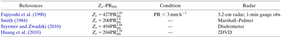
TABLE6-3.Ze–PRSNrelationships are given based on earlier studies.

References Ze–PRSN Condition Radar

Fujiyoshi et al. (1990) Ze5427PR1_SN:09 PR,3 mm h21 3.2-cm radar; 1-min gauge obs

Smith (1984) Ze5200PR1_SN:6 — Marshall–Palmer

Szyrmer and Zwadzki (2010) Ze5494PR1_SN:44 — Disdrometer

calculated for each particle type, and then mixing ratio and number concentration are retrieved. He stressed that interacting particle distributions within the cloud should be preserved rather than only number con-centrations. Iguchi et al. (2012) compared the radar reflectivity factors derived using four different com-binations of observations with NWP model predictions of radar reflectivity. Their results are shown inFig. 6-7. This figure suggests that riming processes and bulk versus bin microphysics schemes resulted in signifi-cant difference in reflectivity factor Ze. They also

stated that substantial uncertainties in the mass–size and size–terminal fall velocity relations of snow-flakes significantly affected the results. For the bulk microphysics, they stated that overestimation ofZe

was likely due to substantial deposition growth di-rectly onto snow that was not modeled using the bin scheme.

During the last couple of decades several studies in the literature have focused on retrievals of ice particle properties with polarimetric radars (Zhang et al. 2011a,b;Hogan et al. 2003;Ryzhkov and Zrnic 2007). Polarimetric radar observations can be used to detect cloud physical properties, for example, particle phase, shape, and water content, and hence derive in-formation about processes that play an important role for snow precipitation (Kennedy and Rudledge 2011).

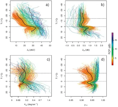
Bechini et al. (2013)used observations from C- and X-band radars in northwestern Italy to study the be-havior of the polarimetric variables in the ice region of precipitating stratiform clouds, with special emphasis on the specific differential phase parameterKdp. They state that stratiform precipitation, irrespective of the precipitation type at the ground and as opposed to convective systems, is characterized by well-pronounced positive differential reflectivity Zdr and Kdpvalues near the model-predicted2158C isotherm (Fig. 6-8). This figure shows the profiles of various polarimetric parameters, including horizontal re-flectivityZh,Zdr,Kdp, and correlation coefficientrHV as a function ofTfor stratiform and convective clouds. The regions of enhancedZdrandKdpare likely related to the growth of dendrite crystals in the area where the difference between the saturation vapor pressure over water and the saturation vapor pressure over ice is greatest.Yuter and Houze (1995)defined a metric for convection called the radar convective parameter (RCP; a simple parameter to describe the degree of convection in a given reflectivity vertical profile) that is also plotted on this figure.Bechini et al. (2013)defined stratiform conditions when RCP is lower than the 50th percentile and is convective otherwise. Their work also showed, in stratiform precipitation, that Kdp

observations around the2158C temperature level are well correlated (0.8) with the reflectivity in the un-derlying rain layer.

3) SATELLITE-BASED PRECIPITATION RETRIEVALS

Cloud and snow retrievals can be performed based on active sensors on satellites, for example, radars or direct measurements of satellite passive spectral channels (Matrosov 2015;Matsui et al. 2013;Iguchi et al. 2012;Rabin et al. 2016).Iguchi et al. (2012)indicated a relatively high correlation of around 0.7 between satellite and WSR-88D IWP retrievals. The mean relative differences between spaceborne and ground-based estimates of IWP were around 50%–60%, which is on the order of IWP retrieval uncertainties and is comparable to the differences among various operational CloudSat IWP products. IWP is an important ice cloud parameter that is routinely retrieved fromCloudSatmeasurements and used to characterize the quantitative evolution of precipitating ice regions. IWP can be estimated in predominantly stratiform precipitation systems that are characterized by a radar bright band, which effectively separates the precipitating ice cloud regions from layers containing rain. The bright band is defined as the cloudy layer where melting and aggregation of ice or snow crystals increases at about 08C, resulting in large reflectivity for melting snow. This happens because of water’s re-flectivity is approximately 9 or 10 times as reflective as ice for the microwave energy range. Therefore these large wet snowflakes will show a high reflectivity (Caylor et al. 1990;

Harrison et al. 2000) that needs to be corrected for accurate precipitation rate–reflectivity relationships.

Multispectral infrared observations obtained from Geostationary Operational Environmental Satellite-13 (GOES-13) can also provide estimates of snowfall on the ground (Rabin et al. 2016). In their work, a new technique is described for identifying clouds capable of producing high snowfall rates and incorporating wind information from the satellite observations. The potential for monitoring snowfall at the surface from estimates of cloud-top temperature and height, phase (water, ice), hydrometer size, optical depth, inferred altitude of the dendritic ice growth zone, horizontal wind patterns near cloud tops, and a GOES precipitation algorithm are evaluated. The time evolution of these satellite estimates are validated using measurements obtained from ground-based in situ and remote sensing platforms during both precipitation events.

Atlas et al. 1995). To meet accuracy requirements, the GPM Core Observatory satellite carries a combina-tion of active and passive microwave sensors with improved capabilities to detect light rain and falling snow. A dual-frequency Precipitation Radar (DPR) on the GPM satellite provides radar observations at both Ku band (13.6 GHz) and Ka band (35.5 GHz) and includes a high sensitivity mode for detection of light/frozen precipitation (Fig. 6-9). The GPM Mi-crowave Imager (GMI) includes 10–89- and 166– 183-GHz channels (Fig. 6-9). These sensor upgrades require more complex precipitation algorithms that harness multisensory and multifrequency satellite signals to estimate warm-/cold-/mixed-phase pre-cipitation rates over various prepre-cipitation regimes. The GPM simulator, which is based on forecasting

model products, can be used as a tool for radiance-based precipitation microphysics evaluation and assimilation methods (e.g.,Matsui et al. 2009;Li et al. 2010;Han et al. 2013). The GPM satellite simulator translates the Weather Research and Forecasting Model with Spec-tral Bin Microphysics (WRF-SBM) simulated geo-physical parameters (Iguchi et al. 2012;Li et al. 2005) into the GPM satellite products for validation applications. The WRF-SBM features explicit size-bin-resolving cloud mi-crophysics rather than the bulk mimi-crophysics used in the previous satellite applications.

5. Snow precipitation prediction

In this section, processes and issues related to snow prediction based on numerical models are summarized.

FIG. 6-8. Hourly vertical profiles of C-band (a) horizontal reflectivityZh, (b) differential reflectivityZdr,

(c) differential phase shiftKdp, and (d) correlation coefficientrHVcolored according to their respective RCP

values. The RCP quantiles (0%, 25%, 50%, 75%, and 100%) represent values of 1.1, 2.7, 3.9, 7.3, and 21.7 dB, respectively. The black (gray) thick lines represent the average of the daily profiles for stratiform (convective) events. To highlight the variations for small values, theKdpprofiles are plotted on a log axis (adapted from

a. Processes affecting snow precipitation

Cloud microphysical processes determine the type and amount of precipitation at the surface. Although there have been significant developments over the last 50 years, it is still challenging to predict cloud micro-physics properties and snow precipitation with fore-casting models because of the issues related to measurements used to derive physical parameteriza-tions. The major issues with snow precipitation involve in-cloud microphysical processes such as ice nucle-ation, ice crystal growth, collision–aggregation pro-cesses, riming, secondary ice crystal production, and freezing and melting, as well as dynamical processes such as mixing and turbulence.

Ice nucleation [seeKanji et al. (2017, chapter 1) and

Gultepe et al. (2017, chapter 4)] parameterizations have important effects on PSDs that occur mainly in two ways: (i) heterogeneous nucleation and (ii) ho-mogeneous nucleation (Gultepe et al. 2016). There are different mechanisms by which heterogeneous ation occurs as follows: 1) deposition/freezing nucle-ation, 2) contact nuclenucle-ation, 3) immersing nuclenucle-ation, and 4) secondary ice nucleation. Homogeneous nucle-ation happens at temperatures less than about2388C. Heterogeneous nucleation occurs because of the exis-tence of INPs that can affect the precipitation amount and rate at the surface. Anthropogenic aerosol can also potentially play a role as heterogeneous ice nucleating particles and affect precipitation For instance, increasing INP concentrations may lead to more but smaller ice crystals (for the same ice water content) that suppresses snow amount but increases cloud cover (Zubler et al.

2011;Saleeby et al. 2013). On the other hand, for the case of reduced INP concentration within convective clouds, aerosols can play a different role, potentially leading to increasing precipitation (Rosenfeld and Lensky 1998;

Williams and Stanfill 2002;Xu 2013) as a result of newly formed ice crystals, followed by collision–coalescence and aggregation processes. Secondary ice production (Field et al. 2017, chapter 7) can also modify the PSD through the production of large numbers of small ice crystals.

The uncertainties associated with the in-cloud sedi-mentation of hydrometeors are related to the micro-physical characteristics of solid and liquid water particles such as particle size, habit, and water amount. These parameters are related to particle terminal ve-locity and mass, as well as updrafts and turbulence. In convective clouds, vertical air velocity and turbulence play a major role in particle growth as they impact both riming and aggregation while they grow by vapor diffu-sion (Kajikawa and Heymsfield 1989). Particle densities are related to particle habit and temperature that affect precipitation type, rate, and amount extensively. Pre-cipitation in NWPs and cloud models occurs as a function of the assumed threshold value of crystal size and/or IWC (or LWC) in a model process that is called autoconversion and that represents the coalescence of small cloud parti-cles (ice or liquid) to form larger precipitation-sized par-ticles. During an autoconversion process, excessive cloud water or cloud ice beyond the threshold values is con-verted to falling snow (Gultepe et al. 2016). For auto-conversion of cloud water to rain, it is usually assumed that droplets are larger than 40–50mm, whereas for au-toconversion of ice crystals to snow, ice crystals are

assumed to be larger than 200–500mm (Khairoutdinov and Kogan 2000;Gultepe et al. 2015). The representation of autoconversion processes in NWP and climate models are still subject to large uncertainty especially for snow precipitation, and needs to be better evaluated. In the last section in this chapter, this issue will be clarified with new suggested methods that focus on the prediction of the evolution of particle properties (e.g., Harrington et al. 2013a,b;Morrison and Milbrandt 2015).

b. Prediction of snow precipitation

Numerical modeling of snow precipitation can be challenging because of the complex microphysical processes that occur within cloud systems. Assump-tions used in microphysical parameterization algo-rithms in NWP and climate simulations should be tested by comparing observations and model simulations.

The majority of microphysics parameterizations can be classified based on how they treat the size distribution for each particle category. Bin-resolving schemes dis-cretize the PSD of each hydrometeor category into a finite number of size or mass bins and predict changes to the distribution by predicting changes to the number (and sometimes also mass) of particles in each bin. No functional form of the PSD is assumed and if the number of bins is large enough, details of the PSD can be well resolved. The driving model must advect the predicted number (and mass) in each bin. Bin schemes are very computationally expensive, particularly in 3D models, and with current computational power, they can only be used in research mode.

For the bulk microphysics approach, each PSD is assumed to have a specific functional form, such as a gamma distribution or lognormal distribution. Many schemes assume a three-parameter complete gamma distribution (which reduces to an inverse-exponential distribution for a shape parameter value of zero). Changes to the PSD are modeled by predicting changes to one or more parameters that describe the function. One or more moments of the distribution are then predicted, which in turn result in changes to the dis-tribution parameters. For each prognostic moment, there is a degree of freedom (i.e., an independently varying PSD parameter). The changes to the moments are computed as the sum of the changes due to each parameterized microphysical processes where each process rate is essentially computed by taking the growth rate for a particle of a given size or mass, mul-tiplying by the PSD, integrating over all sizes, and re-lating the integral quantity to the prognostic moment. The prognostic moments are normally related to physical quantities such as the total mass or number

concentration; other quantities such as reflectivity can also be used in a similar way. Because of the re-duced number of prognostic variables used in bulk microphysics schemes compared to bin schemes, and the low cost of computational advection and diffu-sion used by the dynamical model, as well as the schemes themselves, bulk schemes (Tiedtke 1993;

Del Genio et al. 1996;Sundqvist et al. 1989) in op-erational NWP and climate prediction models are preferred for precipitation prediction relative to detailed bin microphysics schemes (e.g.,Onishi and Takahashi 2012).

The PSDs of precipitation particles such as rain, snow, and graupel are usually assumed to have a simple ex-ponential form (Iguchi et al. 2012), as

N(D)5N_oexp(2lD) , (6-10)

where D is the particle diameter, l the slope pa-rameter, andNois the intercept parameter. The mass

and terminal velocities for each particle type are described as a function of particle diameter.Eito and Aonashi (2009)used two-moment bulk microphysics scheme to study frozen hydrometeor properties simulated by the JMA-NHM and calculated the slope parameter as

l_S,R,G5 prsNoS,R,G r_aq_S,R,G

!0:25

, (6-11)

whereqis the mixing ratio with subscripts for snow (S), rimed particles (R), and graupel (G),rais the air

density, and rs is the snow density. The No is the

prescribed number concentration of particles or it can be obtained through the slope parameter when an exponential PSD is assumed. The D parameter is usually defined in terms of maximum size of ice crystals when ice microphysical parameters are de-termined (McFarquhar and Black 2004). The empir-ical equations for mass–size relationships are usually prescribed; therefore, they need to be specified for various particle types. In addition to processes of vapor diffusion and ice nucleation, accretion, colli-sion and coalescence, riming, breakup, and aggrega-tion processes through autoconversion, affect the amount of falling snow. The presentation of all of these processes use constant coefficients that are poorly known.

1994) that represent the mass conservation of snow (SN) crystals as

P_SN5P_SAUT1P_SACI1P_SACW1P_SFW1P_SFI1P_RACI

1P_IACR1P_GACS1P_GAUT1P_RACS1P_SACR 1P_SSUB1P_SDEP.

(6-12) All the components for snow production [Eq. (6-12)] such as ice nucleation, vapor diffusion, aggregation, riming, and autoconversion are described inTable 6-4

and are based on several assumptions related to their physical characteristics (e.g., mass–length relationships, particle size distributions, fall velocities, collection effi-ciencies); hence, these play an important role for snow precipitation prediction (Tomita 2008). All of the pro-cesses given in Eq. (6-12) can be formulated as pro-portional to moments of the snow size distribution. Some approaches simply use prognosed moments such as ice water content combined with atmospheric variables such as temperature (for a single-moment scheme) to directly predict the moments required for each process. In this way the PSD information is implicit in moment prediction equations (Thompson et al. 2008;

Field et al. 2007).

6. Precipitation efficiency

Precipitation efficiency [Peff(h21)] is defined by the ratio of the observed precipitation on the ground to the possible precipitation flux within the cloud that is the product of total water content (TWC; ex-cluding vapor amount) andVf, representing the entire

cloud system (Sui et al. 2007;Gultepe 2015). Here, it is defined as

P_eff5 PR V_fTWC

C

Dt, (6-13)

where PR (kg m22h21) is the precipitation rate at the surface, TWC (kg m23] is the total condensed water content,Vf(m s21) is mass concentration weighted fall

velocity within the cloud,Cis the conversion factor for time (1/3600), andDt(h) is the time period. Note that this ratio has units of inverse time. Therefore it rep-resents the reciprocal of the time scale to remove condensed water via precipitation. ThePeffcan change as a function of numerous atmospheric parameters. ThePeffdeviates from values that would be expected based on adiabatic conditions. For example,Peffcan change from 10% up to 70% except for highly satu-rated orographic convective systems where it becomes nearly 100% as pointed byBrowning et al. (1974,1975)

andSchmidt (1991).Peffcan be calculated differently based on the need of application and some of them are presented below.

Precipitation rate over the orographic areas can be re-lated to the various factors including mountain physical conditions and meteorological parameters. The studies of

Jiang and Smith (2003),Sawyer (1956), and Elliott and Hovind (1964)suggested thatPeffcan change from 20% up to 100% dependent on environmental conditions. Pre-cipitation efficiency over the orographic areas can be influenced by mountain topography in addition to meteo-rological parameters. Variability in weather conditions over mountainous regions can be significant for the short distances along the mountain slopes. Liquid or solid pre-cipitation amount over the slopes may increase or decrease with height, depending on how the thermodynamic con-ditions and atmospheric stability change along these slopes (Gultepe et al. 2015;Gultepe and Zhou 2012;Mo et al. 2014). Knuth et al. (2010) suggested that blowing and drifting snow plays very important roles on the snow depth measurements. They stated that more than half of their observation sites were influenced by these factors and hence precipitation measurements included large un-certainties. Similar issues related to blowing and drifting snow effects on precipitation measurements were also stated byChoularton et al. (2008),Rogers and Vali (1987), andLloyd et al. (2015).

The measurements of meteorological parameters such as precipitation type, amount, intensity, and phase changes along the mountain slopes also play an important role in assessing the model-based predictions of Peff. The model resolution plays an important role for precipitation rate be-cause of inhomogeneity in its distribution (Mailhot et al. 2014). The lower precipitation amounts usually occur with decreasing resolution in the model, and forecasts pre-cipitation rate decreases with increasing grid area size. They

TABLE6-4. The main source and sink terms as subscripts used in the water budget equation [Eq. (6-12)] to estimate snow pre-cipitation amountP.

SAUT Autoconversion of cloud ice to snow SACI Accretion of cloud ice by snow SACW Accretion of cloud water by snow SWF and SFI Rates at which cloud water and cloud ice

transform to snow by deposition and riming, respectively, based on the growth of a 50-mm ice crystal

pointed out that sampling strategies are important for model validation studies and precipitation assess-ment. Therefore, the model simulations should be done with the appropriate time and space scales, re-solving the physical processes. Jiang and Smith (2003), using a mesoscale numerical model with a 3D Gaussian-type mountain called Advanced Regional Prediction System (ARPS), studiedPeffover an orographic region. If

^

sc represents an assumed specific condensate rate and^s

the measured condensate rate, then R(^sc/^s) (Jiang and Smith 2003) is provided as

R5g

ffiffiffiffiffiffiffiffiffiffiffiffiffiffiffiffiffiffiffiffiffi pq_vs(0)h_m

p

D(t21

a 1t2f1)

, (6-14)

whereDis the model box height,tfis the fallout time

scale,gis the collection factor,tais the advection time

scale,qvs(0) is the saturation vapor mixing ratio at the surface, andhmis the mountain height. Assuming these

as 1 km, 1000 s, 0.5 s21, 1000 s, 2 g kg21, correspondingly, the criticalhmshould be 500 m to makeR51 (Jiang and Smith 2003). Changing from a nonprecipitating to pre-cipitation stage,Rshould increase by either decreasing

^

scor increasing^sas suggested byJiang and Smith (2003).

A relationship between Peff andRover the windward side of the mountain is given as

P_eff5 121

R

11tf

t_a

. (6-15)

The results obtained based on Eq. (6-15) suggest that Peffincreases from 0% to 40% with increasingRfrom 1 to 5, nonlinearly. The value of R can increase by mountain height,qvs, advection time, increasing collec-tion factor, fallout time, increasing horizontal wind speed, and decreasing mountain width.

ThePeffcan also be defined based on modeling needs such as obtaining precipitation intensity from a forecast model. Braham (1952) used the influx of water vapor into the storm base as the rainfall source, and defined it as the ratio of PR to the sum of precipitation source terms, representing large-scale precipitation efficiency (LSPeff). This definition as indicated by Li and Gao

(2011)is used by many others in the forecasting models (Ferrier et al. 1996;Tao et al. 2004;Sui et al. 2005;2007), and details of this subject can be found in Li and Gao (2011). Based on cloud microphysical schemes,Peff us-ing microphysical budget source terms (Sui et al. 2005) is also defined as cloud microphysics precipitation effi-ciency (CMPeff) (Li et al. 2002;Sui et al. 2005). Snow precipitation efficiency, as described in budget terms for snow precipitation, can also be defined similarly.

7. Snow precipitation effects on weather, climate, and society

In this section, snow precipitation effects on weather, climate, and society are studied.

a. Weather

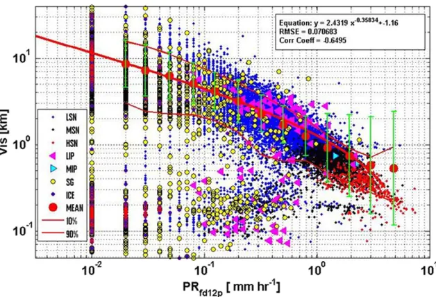
Snow precipitation is an important parameter affect-ing weather processes within and below the cloud. It affects visibility, temperature, and surface weather conditions such as flooding and cooling processes. Its intensity at the surface is related to falling snow crystal size and habit distributions, as well as particle fall velocity. For example, snow intensity can be pa-rameterized based on characteristic snow crystal size, crystal density, and Vis (Gultepe et al. 2016) as

PR_SN(mm h21)5Ar_iD_oV_t/Vis , (6-16)

whereAis 4.683104andDois the median diameter. This

equation is similar to that ofRasmussen et al. (1999). The effect of snow precipitation on visibility is crucial for aviation and transportation applications (Gultepe et al 2014a;Stoelinga and Warner 1999).Figure 6-10 shows Vis versus snow PRSNobservations for various particle shapes based on ground-based FD12P present weather sensor observations. The fit equation given in the figure with standard deviations indicates the var-iability of Vis versus PR for various snow types.

To assess the SN impact on weather processes, the en-ergy equivalent of PR can also be considered. According to the energy conservation budget, a relationship between PRSN(mm day21) and its equivalent energy amount Qe(W m22) due to sublimation can be obtained as

Q_e5K_cPR_SNL_ice, (6-17)

whereKcis a conversion constant of 1/86 400 day, and

Lice(J kg21) is the latent heat of sublimation. When the surface is covered by snow, energy taken from surrounding air for evaporation of ice crystals (sublimation) is more than required for a surface covered by water (Barry 1981). UsingLiceat 08C as 2.833106J kg21and assuming PR51 mm day21_{occurring over the Arctic regions,Q}

e

becomes 32.8 W m22. This suggests that latent heat is released at cloud levels by condensation and consumed by sublimation of snow crystals at the surface. Both ef-fects modify the outgoing infrared radiative fluxes that result in net cooling at the surface.

b. Climate

moisture budgets, and cloud water budget terms. Ice clouds in the atmosphere can modify IR heating and cooling profiles. Falling snow crystals results in cooling at higher levels after decreasing cloud amount (dehumidify the cloud layer) and IR cooling at the surface. Evapora-tive cooling at the surface due to absorption of heat from environment also occurs. Observations collected by snow precipitation sensors can be used to provide climatolog-ical trends after removal of wind effects. A LPM dis-drometer during the entire SAAWSO project, which took place in the sub-Arctic, was used to assess the LSN impact on snow occurrence (Gultepe et al. 2016).

Figure 6-11 shows a probability density function (pdf) plot for PRSNover the entire SAAWSO project that in-cludes heavy snow (HSN) conditions that occurred over an ;1-yr time period, representing winter conditions (Gultepe et al. 2016). The fit equation for the pdf of snow PR based on the Weibull distribution is obtained as

pdf50:2a b

_x

a

b

e2xb/a, (6-18)

wherexis the PR,a50.3407,b50.67, and 0.2 is the nor-malization factor for the fit.Figure 6-11suggests that LSN PR,0.5 (1.0) mm h21occurred 75% (87%) of the time and the corresponding PA represented 11% (20%) of the total. The global distribution of snowfall is very important for climate studies because of its effect on the hydrological cycle (Löhnert et al. 2011;Tapiador et al. 2012), and it is strongly related to climate change. Low precipitation

rates, low temperatures, and strong wind effects can make accurate snowfall measurements a challenge. Pre-vious studies (Rasmussen et al. 1999;Gultepe et al. 2015) suggested that the main challenges in adequately mea-suring snowfall are the high spatial and temporal

FIG. 6-10. FD12P Vis vs PR for all snow events occurred during the FRAM Science of Nowcasting Winter Weather for Vancouver 2010 (SNOW-V10) project for various pre-cipitation types shown in the legend (adapted fromGultepe et al. 2014a,b). The symbols as LSN, MSN, HSN, LIP, MIP, SG, and ICE represent light snow, moderate snow, heavy snow, light ice crystal precipitation, snow grains, and ice crystals, respectively.

variability as well as the enormous complexity of snow crystal habit, density, and PSD. Accurate surface-based snowfall measurements are only sporadically available in the northern regions. Therefore, satellite remote sensing methods are needed to estimate LSN amount and rate but these methods lack sensitivity to low LSN PR.

Global precipitation measurements, including methods, uncertainty, datasets, and applications related to snow measurements, were studied byGruber and Levizzani (2008),Rudolf and Rubel (2005), andTapiador et al. (2012). These studies concluded that LSN measure-ments and its prediction may include large uncer-tainties that can affect validation of model simulations with observations.Figure 6-12shows that precipita-tion changes are up to 50% in many regions of world, and it is likely that climate change will result in quick melting of snow on the ground; therefore, snow science and research need to be further explored for polar conditions.

Overall, snow precipitation processes are important for climate change assessment, the hydrological cycle, NWP model validations, and aviation applications. The LSN (defined as PR,0.5 mm h21) precipitation in cold climates usually cannot be measured accurately be-cause of instrumental issues; sensor calibrations un-available for cold weather conditions, and unreliable response of the optical sensors to the cold and harsh environments (Gultepe et al. 2016).

c. Society

Snow precipitation can affect society through the in-terruption of commercial flights (Gultepe et al. 2016;

Rasmussen et al. 1999) and other impacts on trans-portation, sporting activities (Doyle 2014;Mo et al. 2014), modifying the water levels in reservoirs (Jorg-Hess et al. 2015;Gurtz et al. 2003;Jonas et al. 2009), and modifying the water levels available for ecosystems (Semple 1918;

Essery et al. 2009;Liston 1999). These suggest that accu-rate prediction of changes in snow precipitation is needed. As pointed out above, prediction of snow rate and amount are related to both in-cloud and ground-level microphys-ical, dynammicrophys-ical, and radiative processes. Therefore, more frequent and accurate measurements are needed in order to better understand and resolve these processes over the smaller scales (e.g., less than a few kilometers).

8. Challenges for understanding snow precipitation

The major challenges for improving snow pre-cipitation predictions are related to gaps in our un-derstanding of in-cloud processes (section 5) and surface snow measurements (section 3). Both issues affect modeling aspects of snow precipitation, including those

for both weather forecasting and climate modeling, and they are summarized below.

a. Measurement issues

The major issues with snow measurements are related to instrumental sensitivity and collection efficiency of snow crystals when environmental conditions change, for example, increasing wind speed and turbulence (Gultepe et al. 2016). Bogdanova et al. (2002) analyzed Arctic precipitation events and found that annual mean false precipitation detection makes up 30% or more of the total measured precipitation. In their work it is stated that blowing snow and blizzards significantly affect the quality of the in situ snow measurements (e.g., in coastal high-latitudinal regions, ice sheets, tundra, mountain desert, and steppe climatic zones), resulting in false precipitation detection. Unfortunately, light SN measurements cannot be measured accurately with weighing gauges such as Geonor or Pluvio (Gultepe et al. 2014a,b,2016). Light snow PR is usually calculated by the measurements of OPWS (such as Vaisala PWD or Metek SWS) because of their lower threshold values for snow detection (0.01 mm h21) compared to the TPS and Geonor lower threshold of 0.5 mm h21 without wind corrections (Rasmussen et al. 2012). Because of high winds and strong turbulence, error in SN measurements based on TPS can be large (Boudala et al. 2014). Above works suggest that measurement issues are still important over their evaluations in the cold climates and Arctic regions, and these are now summarized below.

1) LIGHT SNOW MEASUREMENTS

The contribution of light snow precipitation amount, including ice crystals from clouds, ice fog crystals, and diamond dust particles, is important for hydrological assessment and weather applications (Gultepe et al. 2007,2015,2016;Girard and Blanchet 2001a,b;Yang et al. 2005;Huffman et al. 1995;Intrieri and Shupe 2004). Although heavy precipitation with large particles brings in large amounts of water over land and ocean surfaces, continuous light pre-cipitation can play a much more important role in the growing season of plants, on aviation mission plan-ning, and on the assessment of climate change. The LSN precipitation can also be responsible for dis-crepancies in precipitation retrievals between remote sensing platforms and in situ observations, and be-tween model-based predictions and in situ–based observational analysis results. Gultepe et al. (2016)

shows that the GCIP sensor was much more sensitive to missing snow precipitation compared to others. These results suggested that light snow measurements need to be improved significantly.

2) CATCH EFFICIENCY AND BIAS FOR SNOW MEASUREMENTS

Catch efficiency, defined as the ratio of snow mea-surements to reference sensor meamea-surements (e.g.,

DFIR), is obtained as a function of wind speed that is an important parameter to be considered for making accurate measurements of snow amount. Zhang et al. (2015)state that uncertainty in Geonor measurements can be about 44% whenUhis between 0.5 and 3.5 m s21, but

whenUh.3.5 m s21the Geonor could not measure any

light snow. Bias corrections of snow measurements for weighing gauges can be related to wind-induced under-catch, wetting loss, and evaporation loss (Sevruk and FIG. 6-12. Precipitation change (%) from the period 1980–99 to 2080–99 in the Consortium for the Application of