Identification of a heterogeneous orthotropic conductivity in a rectangular domain

This is a repository copy of Identification of a heterogeneous orthotropic conductivity in a rectangular domain.

White Rose Research Online URL for this paper: http://eprints.whiterose.ac.uk/91459/

Version: Accepted Version

Article:

Hussein, MS, Lesnic, D and Ivanchov, MI (2017) Identification of a heterogeneous orthotropic conductivity in a rectangular domain. International Journal of Novel Ideas:Mathematics, 1. ISSN 2331-5210

[email protected] https://eprints.whiterose.ac.uk/ Reuse

Unless indicated otherwise, fulltext items are protected by copyright with all rights reserved. The copyright exception in section 29 of the Copyright, Designs and Patents Act 1988 allows the making of a single copy solely for the purpose of non-commercial research or private study within the limits of fair dealing. The publisher or other rights-holder may allow further reproduction and re-use of this version - refer to the White Rose Research Online record for this item. Where records identify the publisher as the copyright holder, users can verify any specific terms of use on the publisher’s website.

Takedown

If you consider content in White Rose Research Online to be in breach of UK law, please notify us by

Identification of a heterogeneous orthotropic

conductivity in a rectangular domain

M.S. Hussein1,2_{, D. Lesnic}1 _{and M.I. Ivanchov}3

1_{Department of Applied Mathematics, University of Leeds, Leeds LS2 9JT, UK}

2_{Department of Mathematics, College of Science, University of Baghdad, Baghdad, Iraq} 3_{Faculty of Mechanics and Mathematics, Department of Differential Equations, Ivan}

Franko National University of Lviv, 1, Universytetska str., Lviv, 79000, Ukraine

E-mails: [email protected], [email protected] (M.S. Hussein),

[email protected] (D. Lesnic), [email protected] (M.I. Ivanchov).

Abstract

This paper investigates the problem of identifying a heterogeneous transient orthotropic thermal conductivity in a two-dimensional rectangular domain using initial and Dirichlet boundary conditions and fluxes as overdetermination conditions. The measurement data represented by the heat fluxes are shown to ensure the unique solvability of the inverse problem solution. The finite-difference method is employed as the direct solver which is fed iteratively in a nonlinear minimization routine. Exact and noisy input data are inverted numerically. Numerical results indicate that accurate and stable solutions are obtained.

Keywords: Heat equation; Orthotropic material; Inverse problem

1

Introduction

The determination of coefficients in inverse heat conduction problems for the parabolic heat equation, [9], continues to receive significant attention in a variety of fields, such as heat transfer, oil recovery, groundwater flow, and finance. Many researchers investigated the case of simultaneous identification of coefficients in two-dimensional heat conduction problems, [3, 4, 13].

The identification of physical properties such as thermal conductivity using measured temperature or heat flux values at well sites is an important inverse problem. A common identification strategy is the indirect one where one can minimize the gap between a computed solution and the measured data (observations) via an iterative process, [12].

The main obstacle in this kind of problem is that there are usually so few observations that one finds hard to evaluate the spatial derivative of temperature by simple numerical differentiation. Therefore, heavier and more time-consuming optimization techniques are needed to obtain reliable results.

The estimation of thermal properties for the multi-dimensional inhomogeneous and anisotropic media is rather scarce in the literature [1, 7]. The aim of the present study is to consider a two-dimensional coefficient identification problem to estimate the space and time varying principal direction components of an orthotropic conductivity in a rectan-gular domain.

constrained nonlinear minimization problem that has to be solved using the MATLAB routinelsqnonlin. In Section 7, numerical results are presented and discussed and finally conclusions of the paper are given in Section 8.

2

Statement of the inverse problem

Consider the nonlinear inverse coefficient identification problem which requires determin-ing the principal direction components a(y, t)>0 and b(x, t)>0 of the two-dimensional heterogeneous orthotropic rectangular mediumD= (0, h)×(0, ℓ) together with the tem-peratureu(x, y, t) satisfying the heat equation

ut=a(y, t)uxx+b(x, t)uyy+f(x, y, t), (x, y, t)∈QT :=D×(0, T), (1)

wheref is a given heat source, subject to initial, boundary and overdetermination condi-tions

u(x, y,0) =ϕ(x, y), (x, y)∈D, (2)

u(0, y, t) = µ1(y, t), u(h, y, t) =µ2(y, t), (y, t)∈[0, l]×[0, T], (3)

u(x,0, t) =µ3(x, t), u(x, l, t) =µ4(x, t), (x, t)∈[0, h]×[0, T], (4)

a(y, t)ux(0, y, t) = µ5(y, t), (y, t)∈[0, l]×[0, T], (5)

b(x, t)uy(x,0, t) =µ6(x, t), (x, t)∈[0, h]×[0, T]. (6)

In the above setting one can see that Cauchy data are prescribed over the boundariesx= 0 and y = 0. Also by restricting the conductivity components a(y, t) and b(x, t) be inde-pendent ofx and y, respectively, it then makes sense to study the injectivity/surjectivity of the mapping (a, b) 7→ (µ5, µ6). We finally mention that in the general case when

a(x, y, t) and b(x, y, t) depend on all coordinates then the right hand side of (1) modifies

as (a(x, y, t)ux)x+ (b(x, y, t)uy)y+f(x, y, t).

There is no theory available for this general orthotropic inverse coefficient identifica-tion, but at least in the isotropic case when a=b, all the knowledge of the temperature

u(x, y, t) for (x, y, t)∈ QT is necessary in order to render a unique solution, [5]. All this

discussion warrants and justifies our assumption that a(y, t) and b(x, t) are independent on the variables x and y, respectively. Then, the measurements (5) and (6) are supplied as the correct traces of functionals, according to the illuminating discussion of Cannon et al. [2].

Suppose that the following assumptions hold:

(A1) ϕ ∈ C2+γ_{(D), µ}

i ∈ C2+γ,1+γ/2([0, l]× [0, T]), i ∈ {1,2}, µk ∈ C2+γ,1+γ/2([0, h]×

[0, T]), k ∈ {3,4}, µ5 ∈Cγ,γ/2([0, l]×[0, T]), µ6 ∈Cγ,γ/2([0, h]×[0, T]), f ∈Cγ,γ/2(QT)

for some γ ∈(0,1);

(A2) ϕx(x, y) > 0, ϕy(x, y) > 0,(x, y) ∈ D, µ5(y, t) > 0,(y, t) ∈ [0, l]×[0, T], µ6(x, t) >

0,(x, t)∈[0, h]×[0, T];

(A3) consistency conditions of the zero and the first orders.

We remark that a formal elimination ofa(y, t) andb(x, t) in (5) and (6), respectively, and substitution into (1) result in the nonlinear partial differential equation

ut(x, y, t) =

µ5(y, t)

ux(0, y, t)

uxx+

µ6(x, t)

uy(x,0, t)

to be solved for the temperature u(x, y, t) subject to the initial and boundary conditions (2)–(4).

3

Existence of solution of the inverse problem

Theorem 1. Suppose that the assumptions (A1)-(A3) hold. Then for some T0 ∈(0, T]

there exists a solution of the problem (1)-(6) such that (a, b, u)∈ Cγ,γ/2_{([0, l]×[0, T} 0])×

Cγ,γ/2_{([0, h]×[0, T}

0])×C2+γ,1+γ/2(QT0), a(y, t)>0,(y, t)∈[0, l]×[0, T0], b(x, t)>0,(x, t)∈

[0, h]×[0, T0].

Proof. In order to make the initial and boundary conditions (2)–(4) homogenous the following notation will be used:

ψ(x, y, t) :=µ1(y, t)−µ1(y,0) +

x

h(µ2(y, t)−µ2(y,0)−µ1(y, t) +µ1(y,0)) +µ3(x, t)−

µ3(x,0)−[µ1(0, t)−µ1(0,0) +

x

h(µ2(0, t)−µ2(0,0)−µ1(0, t) +µ1(0,0))] + y

l[µ4(x, t)−

µ4(x,0)−µ1(l, t) +µ1(l,0)−

x

h(µ2(l, t)−µ2(l,0)−µ1(l, t) +µ1(l,0))−µ3(x, t) +µ3(x,0) +

µ1(0, t)−µ1(0,0) +

x

h(µ2(0, t)−µ2(0,0)−µ1(0, t) +µ1(0,0))].

Then by the superposition

u(x, y, t) =v(x, y, t) +ϕ(x, y) +ψ(x, y, t)

we reduce the equations (1)-(4) to the following ones:

vt =a(y, t)vxx+b(x, t)vyy +F(x, y, t) +a(y, t)(ϕxx(x, y) +ψxx(x, y, t))

+b(x, t)(ϕyy(x, y) +ψyy(x, y, t)), (x, y, t)∈QT, (8)

v(x, y,0) = 0, (x, y)∈D, (9)

v(0, y, t) =v(h, y, t) = 0, (y, t)∈[0, l]×[0, T], (10)

v(x,0, t) =v(x, l, t) = 0, (x, t)∈[0, h]×[0, T], (11)

whereF(x, y, t) := f(x, y, t)−ψt(x, y, t).

Supposing for the moment that the coefficients a(y, t) and b(x, t) are known, we find the solutionv of the problem (8)-(11) as

v(x, y, t) =

t

∫

0 ∫ ∫

D

G(x, y, t, ξ, η, τ)

[

F(ξ, η, τ) +a(η, τ)(ϕξξ(ξ, η) +ψξξ(ξ, η, τ))

+b(ξ, τ)(ϕηη(ξ, η) +ψηη(ξ, η, τ)

]

dξdηdτ, (x, y, t)∈Q_T, (12)

where G(x, y, t, ξ, η, τ) is the Green function of the problem (8)-(11). The assumptions

(A1)-(A3)ensure the existence of such a Green function [8]. Then the solution u of the problem (1)-(4) is given by the formula

u(x, y, t) =ϕ(x, y) +ψ(x, y, t) +

t

∫

0 ∫ ∫

D

G(x, y, t, ξ, η, τ)

[

F(ξ, η, τ) +a(η, τ)(ϕξξ(ξ, η)

+ψξξ(ξ, η, τ)) +b(ξ, τ)(ϕηη(ξ, η) +ψηη(ξ, η, τ))

]

Substituting (13) into (5) and (6) we obtain

a(y, t) =µ5(y, t)

{

ϕx(0, y) +ψx(0, y, t) +

t

∫

0 ∫ ∫

D

Gx(0, y, t, ξ, η, τ)

[

F(ξ, η, τ)

+a(η, τ)(ϕξξ(ξ, η) +ψξξ(ξ, η, τ))

+b(ξ, τ)(ϕηη(ξ, η) +ψηη(ξ, η, τ))

]

dξdηdτ

}−1

, (y, t)∈[0, l]×[0, T], (14)

b(x, t) =µ6(x, t)

{

ϕy(x,0) +ψy(x,0, t) +

t

∫

0 ∫ ∫

D

Gy(x,0, t, ξ, η, τ)

[

F(ξ, η, τ)

+a(η, τ)(ϕξξ(ξ, η) +ψξξ(ξ, η, τ))

+b(ξ, τ)(ϕηη(ξ, η) +ψηη(ξ, η, τ))

]

dξdηdτ

}−1

, (x, t)∈[0, h]×[0, T]. (15)

So, the inverse problem (1)-(6) has been reduced to the system of integral equations (14) and (15).

To begin with, we establish the existence of a positive solution (a(y, t), b(x, t)) of the system of integral equations (14) and (15) in the spaceC([0, l]×[0, T])×C([0, h]×[0, T]) by applying the Schauder fixed-point theorem. For this, we need to find the estimates for the solution. It follows from assumption (A2) that ϕx(0, y) ≥ M1 > 0, y ∈ [0, l], ϕy(x,0) ≥

M2 >0, x∈[0, h]. As the rest of terms in the denominators of (14) and (15) are equal to

zero for t= 0, there existsT0 ∈(0, T] such that the following inequalities hold:

ψ_x(0, y, t) +

t

∫

0 ∫ ∫

D

Gx(0, y, t, ξ, η, τ)

[

F(ξ, η, τ) +a(η, τ)(ϕξξ(ξ, η)

+ψξξ(ξ, η, τ)) +b(ξ, τ)(ϕηη(ξ, η) +ψηη(ξ, η, τ))

]

dξdηdτ

≤

M1

2 ,

ψ_y(x,0, t) +

t

∫

0 ∫ ∫

D

Gy(x,0, t, ξ, η, τ)

[

F(ξ, η, τ) +a(η, τ)(ϕξξ(ξ, η)

+ψξξ(ξ, η, τ)) +b(ξ, τ)(ϕηη(ξ, η) +ψηη(ξ, η, τ))

]

dξdηdτ≤

M2

Then we find from (14) and (15) that

a(y, t)≤A1 :=

max

[0,l]×[0,T]

µ5(y, t)

M1/2

, (y, t)∈[0, l]×[0, T],

b(x, t)≤B1 :=

max

[0,h]×[0,T]

µ6(x, t)

M2/2

, (x, t)∈[0, h]×[0, T], (17)

a(y, t)≥A0 :=

min

[0,l]×[0,T]

µ5(y, t)

max

[0,l] ϕx(0, y) +M1/2

, (y, t)∈[0, l]×[0, T],

b(x, t)≥B0 :=

min

[0,h]×[0,T]µ6(x, t)

max

[0,h] ϕy(x,0) +M2/2

, (x, t)∈[0, h]×[0, T]. (18)

Denoteω := (a(y, t),(b(x, t)) and rewrite the system (14) and (15) as an operator equation

ω =P ω. (19)

Introduce the setN :={ω∈C([0, l]×[0, T0])×C([0, h]×[0, T0]) :A0 ≤a(y, t)≤A1, B0 ≤

b(x, t)≤B1}. It is easy to see that the operatorP mapsN onto N. The compactness of

the operator P may be easily established by the same procedure as in [9].

It follows that the Schauder theorem may be applied to the equation (19) and, hence, there exists a continuous solution of the system of integral equations (14) and (15). Tak-ing into account the assumption (A1), we conclude that a ∈ Cγ,γ/2_{([0, l]×[0, T}

0]), b ∈

Cγ,γ/2_{([0, h] ×[0, T}

0]). Then, it also follows [8] that u ∈ C2+γ,1+γ/2(QT0). The proof is

complete.

Remark. Having the estimates (17) and (18), one can easily estimate from (16) the value of T0.

4

Uniqueness of solution of the inverse problem

Theorem 2. Suppose that µ5(y, t)̸= 0,(y, t)∈[0, l]×[0, T], µ6(x, t)̸= 0,(x, t)∈[0, h]×

[0, T]. Then a solution (a(y, t), b(x, t), u(x, y, t)) of the problem (1)-(6) is unique in the space Cγ,γ/2_{([0, l]×[0, T])×C}γ,γ/2_{([0, h]×[0, T])×C}2+γ,1+γ/2_(Q

T), a(y, t) > 0,(y, t) ∈

[0, l]×[0, T], b(x, t)>0,(x, t)∈[0, h]×[0, T].

Proof. Suppose that there are two solutions (ai(y, t), bi(x, t), ui(x, y, t)), i ∈ {1,2} of the

problem (1)-(6) in the indicated class. Denote a := a1 −a2, b := b1 −b2, u := u1 −u2.

Then (a, b, u) is a solution of the following problem:

ut =a1(y, t)uxx+b1(x, t)uyy+a(y, t)u2xx(x, y, t) +b(x, t)u2yy(x, y, t),

(x, y, t)∈QT, (20)

u(x, y,0) = 0, (x, y)∈D, (21)

u(0, y, t) = u(h, y, t) = 0, (y, t)∈[0, l]×[0, T], (22)

u(x,0, t) =u(x, l, t) = 0, (x, t)∈[0, h]×[0, T], (23)

a1(y, t)ux(0, y, t) = −a(y, t)u2x(0, y, t), (y, t)∈[0, l]×[0, T], (24)

Using the Green function ˜G(x, y, t, ξ, η, τ) of the problem (20)-(23), we find its solution as

u(x, y, t) =

t

∫

0 ∫ ∫

D

˜

G(x, y, t, ξ, η, τ)(a(η, τ)u2ξξ(ξ, η, τ)

+b(ξ, τ)u2ηη(ξ, η, τ))dξdηdτ, (x, y, t)∈QT. (26)

We obtain from (24)-(26) the following integral equations:

a(y, t) =− a1(y, t)

u2x(0, y, t)

t

∫

0 ∫ ∫

D

˜

Gx(0, y, t, ξ, η, τ)(a(η, τ)u2ξξ(ξ, η, τ)

+b(ξ, τ)u2ηη(ξ, η, τ))dξdηdτ, (y, t)∈[0, l]×[0, T], (27)

b(x, t) =− b1(x, t)

u2y(x,0, t)

t

∫

0 ∫ ∫

D

˜

Gy(x,0, t, ξ, η, τ)(a(η, τ)u2ξξ(ξ, η, τ)

+b(ξ, τ)u2ηη(ξ, η, τ))dξdηdτ, (y, t)∈[0, l]×[0, T]. (28)

Note thatu2x(0, y, t)̸= 0, u2y(x,0, t)̸= 0 as (a2, b2, u2) is a solution of (1)-(6) and, hence, it

verifies the conditions (5), (6) with functionsµ5andµ6which do not vanish. Consequently,

(27) and (28) is a homogeneous system of Volterra integral equations of the second kind and has only the trivial solutiona(y, t)≡0, b(x, t)≡0.From this and (20)–(23) we obtain

that u(x, y, t)≡0,(x, y, t)∈Q_T.The proof is complete.

5

Solution of direct problem

In this section, we consider the direct initial boundary value problem (1)–(4) wherea(y, t),

b(x, t), f(x, y, t), ϕ(x, y), and µi, i= 1,2,3,4, are known and the solution u(x, y, t) is to

be determined. To achieve this, we use the Forward-Time-Central-Space (FTCS) finite-difference scheme which is conditionally stable.

We subdivide the solution domain QT into Mx, My and N subintervals of equal step

lengths ∆xand ∆y, and uniform time step ∆t, where ∆x=h/Mx, ∆y=ℓ/My and ∆t=

T /N, for space and time, respectively. At the node (i, j, k) we denote uk

i,j :=u(xi, yj, tk),

wherexi =i∆x,yj =j∆y,tk =k∆t,akj :=a(yj, tk),bki :=b(xi, tk) andfi,jk :=f(xi, yj, tk)

fori= 0, Mx,j = 0, My and k = 0, N.

The simplest explicit difference scheme for equation (1) is given by

uk_i,j+1−uk

i,j

∆t =a

k j

uk

i+1,j −2uki,j +uki−1,j

(∆x)2 +b

k i

uk

i,j+1−2uki,j+uki,j−1

(∆y)2 +f

k

i,j (29)

for i = 1, Mx−1, j = 1, My−1 and k = 0, N. The initial and boundary conditions

(2)–(4) give

u0_i,j =ϕi,j, i= 0, Mx, j = 0, My, (30)

uk_0,j =µ1(yj, tk), ukMx,j =µ2(yj, tk), j = 0, My, k = 1, N , (31)

Let ˜a and ˜b be the maximum values of a(y, t) andb(x, t), respectively, then, the stability condition for the explicit FDM scheme (29) will be [10].

˜

a∆t

(∆x)2 +

˜

b∆t

(∆y)2 ≤

1

2. (33)

The heat fluxes (5) and (6) can be calculated using the second-order FDM approxi-mations:

µ5(yj, tk) =akj

4uk

1,j−uk2,j−3uk0,j

2∆x , j = 1, My−1, k = 1, N , (34)

µ6(xi, tk) =bki

4uk

i,1−uki,2−3uki,0

2∆y , i= 1, Mx−1, k = 1, N . (35)

6

Numerical solution of inverse problem

In this section we aim to obtain stable reconstructions for the principal direction compo-nents a(y, t) > 0 and b(x, t) > 0 of the two-dimensional heterogeneous orthotropic rect-angular medium together with the temperatureu(x, y, t) satisfying the equations (1)–(6). One can remark that at initial timet = 0 the values of the principal direction components are known and they can easily be obtained form the overdetermination conditions (5) and (6) as

a(y,0) = µ5(y,0)

ϕx(0, y)

, b(x,0) = µ6(x,0)

ϕy(x,0)

, y∈[0, ℓ], x∈[0, h]. (36)

The inverse problem is solved based on the nonlinear minimization of the least-squares objective function

F(a, b) :=a(y, t)u_x(0, y, t)−µ₅(y, t)

2

+b(x, t)u_y(x,0, t)−µ₆(x, t) 2

, (37)

or, in discretised form

F(a, b) =

N

∑

k=1

My

∑

j=0 [

aj,kux(0, yj, tk)−µ5(yj, tk)

]2

+

N

∑

k=1

Mx

∑

i=0 [

bi,kuy(xi,0, tk)−µ6(xi, tk)

]2

. (38)

Upper and lower bounds on the thermal conductivities a and b can be specified ac-cording toa priori information on these physical parameters.

In the numerical computation, we take the parameters of the routine lsqnonlin as follows:

• Maximum number of iterations = 105_{× (number of variables).}

• Maximum number of objective function evaluations = 106_{×(number of variables).}

• Solution and objective function tolerances = 10−10_.

The inverse problem (1)–(6) is solved subject to both exact and noisy measurements (5) and (6). The noisy data is numerically simulated as

µϵ51(yj, tk) = µ5(yj, tk) +ϵ1j,k, j = 0, My, k = 1, N , (39)

µϵ₆2(xi, tk) = µ6(xi, tk) +ϵ2i,k, i= 0, Mx, k = 1, N , (40)

whereϵ1j,k and ϵ2i,k are random variables generated from a Gaussian normal distribution

with mean zero and standard deviationσ1 and σ2 given by

σ1 =p× max

(y,t)∈[0,ℓ]×[0,T]|µ5(y, t)|, σ2 =p×(x,t)∈max[0,h]×[0,T]|µ6(x, t)|, (41)

where p represents the percentage of noise. We use the MATLAB function normrnd

to generate the random variables ϵ1 = (ϵ1j,k)_j=0,M

y,k=1,N and ϵ2 = (ϵ2i,k)i=0,Mx,k=1,N as

follows:

ϵ1 =normrnd(0, σ1, My+ 1, N), ϵ2 =normrnd(0, σ2, Mx+ 1, N). (42)

In the case of noisy data (39) and (40), we replace µ5(yj, tk) and µ6(xi, tk) by µϵ51(yj, tk)

and µϵ62(xi, tk), respectively, in (38).

7

Numerical results and discussion

In this section, we present numerical results for the orthotropic thermal conductivity components a(y, t), b(x, t) and the temperature u(x, y, t), in the case of exact and noisy data (39) and (40). To assess the accuracy of the numerical solution we employ the root mean square errors (rmse) defined by:

rmse(a) =

[

1

N(My + 1)

N

∑

k=1

My

∑

j=0

(anumerical(yj, tk)−aexact(yj, tk))2

]1/2

, (43)

rmse(b) =

[

1

N(Mx+ 1)

N

∑

k=1

Mx

∑

i=0

(bnumerical(xi, tk)−bexact(xi, tk))2

]1/2

. (44)

7.1

Example 1

Consider the inverse problem (1)–(6) with unknown coefficients a(y, t) and b(y, t), with the input data ϕ and µi,i= 1,6, as follows:

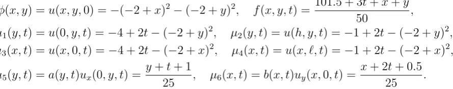
ϕ(x, y) = u(x, y,0) = −(−2 +x)2−(−2 +y)2, f(x, y, t) = 101.5 + 3t+x+y

50 ,

µ1(y, t) = u(0, y, t) =−4 + 2t−(−2 +y)2, µ2(y, t) = u(h, y, t) =−1 + 2t−(−2 +y)2,

µ3(x, t) = u(x,0, t) = −4 + 2t−(−2 +x)2, µ4(x, t) = u(x, ℓ, t) = −1 + 2t−(−2 +x)2,

µ5(y, t) = a(y, t)ux(0, y, t) =

y+t+ 1

25 , µ6(x, t) =b(x, t)uy(x,0, t) =

x+ 2t+ 0.5

25 .

One can remark that conditions of Theorems 1 and 2 are satisfied and therefore, the local solvability of the solution is guaranteed. In fact, it can easily be checked by direct substitution that the analytical solution is given by

a(y, t) = y+t+ 1

100 , (y, t)∈[0,1]×[0,1], (45)

b(x, t) = x+ 2t+ 0.5

100 , (x, t)∈[0,1]×[0,1], (46)

u(x, y, t) =−(x−2)2 −(y−2)2+ 2t, (x, y, t)∈Q_T. (47)

We take a coarse mesh size withN =Mx =My = 5, i.e. ∆x= ∆y= ∆t= 1/5 = 0.2.

Then we need to choose an upper boundU B for aand b such that the stability condition (33) is satisfied. This yields U B = 1/20 = 0.05. Also since a and b represent positive physical quantities we take a lower bound for a and b be given by LB = 0.01. Keeping the sought parameters inside the lower and upper prescribed bounds through all the minimization process increases the performance of identification, [6].

We start our investigation for simultaneously determining the principal direction com-ponents a(y, t) and b(x, t) in a heterogeneous orthotropic with the case of exact input data, i.e. p = 0 in (41). To test the robustness of the iterative method with respect to the independence on the initial guess, we take three different initial guesses namely:

initial A:a0 =aexact+ 3×10−4randn(size(a)), b0 =bexact+ 3×10−4randn(size(b)),

initial B:a0 =aexact+ 3×10−3randn(size(a)), b0 =bexact+ 3×10−3randn(size(b)),

initial C:a0 = ones(size(a)), b0 = ones(size(b)).

where randn(:) is a MATLAB function.

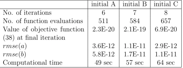
Figure 1 shows the convergence of the objective function (38) with exact input data (5) and (6) for the various initial guesses A, B and C. Table 1 gives more details of these computations including the computational time and thermsevalues (43) and (44). From Figure 1 and Table 1, it can be seen that, as expected, the farther the initial guess is, e.g. initial C, the more iterations and longer computational time are required to achieve convergence. However, for all initial guesses, the objective function (38) converges to the same very small minimum value of O(10−20_{). This shows robustness with respect to the}

0 1 2 3 4 5 6 7 8 10−20

10−15 10−10 10−5 100

Number of Iterations

Objective function

Initial A initial B initial C

Figure 1: The objective function (38) with no noise, for various initial guesses, for Example 1.

Table 1: Number of iterations, number of function evaluations, value of the objective function (38) at final iteration, thermse values and the computational time, with no regularization and no noise for Example 1 for various initial guesses.

initial A initial B initial C No. of iterations 6 7 8 No. of function evaluations 511 584 657 Value of objective function

(38) at final iteration

2.3E-20 2.1E-19 6.9E-20

rmse(a) 3.6E-12 1.1E-11 2.9E-12

0 0.5 1 0 0.5 1 0.01 0.015 0.02 0.025 0.03 t Exact solution y a(y,t) 0 0.5 1 0 0.5 1 0.01 0.015 0.02 0.025 0.03 t Numerical solution y a(y,t) 0 0.5 1 0 0.5 1 0 2 4 6 8

x 10−8

t y

Relative error (%)

(a) 0 0.5 1 0 0.5 1 0 0.01 0.02 0.03 0.04 t Exact solution x b(x,t) 0 0.5 1 0 0.5 1 0 0.01 0.02 0.03 0.04 t Numerical solution x b(x,t) 0 0.5 1 0 0.5 1 0 1 2 3 4

x 10−7

t x

Relative error (%)

(b)

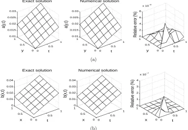
Figure 2: The exact solution (left), numerical solution (middle), error between them (right), with initial guess C, for: (a)a(y, t) and (b) b(x, t), with no noise, for Example 1.

In what follows, we take the initial guess for the unknown coefficients equal to the constant matrix of ones, i.e. we choose the initial guess C. The numerically obtained results foraand bare illustrated in Figure 2 and an excellent agreement can be observed. Next we consider the case of noisy data (39) and (40) with p ∈ {1,5,10}%. The numerically obtained results are illustrated in Figures 3–5 for p = 1%, 5% and 10%, respectively, and summarised in Table 2. From these figures and table it can be seen that as the percentage of noise p decreases from 10% to 5% and then to 1% the numerically obtained solution becomes more stable and accurate.

Table 2: Number of iterations, number of function evaluations, value of the objective function (38) at final iteration, thermse values and the computational time, withp∈ {1,5,10}% noise, for Example 1.

p= 1% p= 5% p= 10% No. of iterations 8 8 8 No. of function evaluations 657 657 657 Value of objective function

(38) at final iteration

2.4E-20 3E-20 7.4E-20

rmse(a) 4.2E-4 0.0021 0.0043

rmse(b) 3.3E-4 0.0017 0.0034

0 0.5 1 0 0.5 1 0.01 0.015 0.02 0.025 0.03 t Exact solution y a(y,t) 0 0.5 1 0 0.5 1 0.01 0.015 0.02 0.025 0.03 t Numerical solution y a(y,t) 0 0.5 1 0 0.5 1 0 2 4 6 8 t y

Relative error (%)

(a) 0 0.5 1 0 0.5 1 0 0.01 0.02 0.03 0.04 t Exact solution x b(x,t) 0 0.5 1 0 0.5 1 0 0.01 0.02 0.03 0.04 t Numerical solution x b(x,t) 0 0.5 1 0 0.5 1 0 2 4 6 t x

Relative error (%)

(b)

Figure 3: The exact solution (left), numerical solution (middle), error between them (right), for: (a)a(y, t) and (b) b(x, t), with p= 1% noisy data, for Example 1.

0 0.5 1 0 0.5 1 0.01 0.015 0.02 0.025 0.03 t Exact solution y a(y,t) 0 0.5 1 0 0.5 1 0.01 0.02 0.03 0.04 t Numerical solution y a(y,t) 0 0.5 1 0 0.5 1 0 10 20 30 40 t y

Relative error (%)

(a) 0 0.5 1 0 0.5 1 0 0.01 0.02 0.03 0.04 t Exact solution x b(x,t) 0 0.5 1 0 0.5 1 0 0.01 0.02 0.03 0.04 t Numerical solution x b(x,t) 0 0.5 1 0 0.5 1 0 5 10 15 t x

Relative error (%)

(b)

0 0.5 1 0 0.5 1 0.01 0.015 0.02 0.025 0.03 t Exact solution y a(y,t) 0 0.5 1 0 0.5 1 0.01 0.02 0.03 0.04 t Numerical solution y a(y,t) 0 0.5 1 0 0.5 1 0 20 40 60 80 t y

Relative error (%)

(a) 0 0.5 1 0 0.5 1 0 0.01 0.02 0.03 0.04 t Exact solution x b(x,t) 0 0.5 1 0 0.5 1 0 0.01 0.02 0.03 0.04 t Numerical solution x b(x,t) 0 0.5 1 0 0.5 1 0 10 20 30 t x

Relative error (%)

(b)

Figure 5: The exact solution (left), numerical solution (middle), error between them (right), for: (a)a(y, t) and (b) b(x, t), with p= 10% noisy data, for Example 1.

8

Conclusions

The inverse problem concerning the identification of the principal direction thermal con-ductivity components a(y, t) and b(x, t) of an orthotropic material and the temperature

u(x, y, t) in the two-dimensional heat equation in a rectangular domain has been

investi-gated. The additional conditions which ensure a unique solvability of solution are given by the heat fluxesµ5 and µ6. The direct solver based on an explicit finite difference scheme

has been developed. The inverse solver based on a nonlinear least-squares minimization has been solved using the MATLAB toolbox routinelsqnonlin. For both exact and noisy data, the numerical results obtained are accurate and stable.

Acknowledgments

M.S. Hussein would like to thank the financial support received from the Higher Com-mittee for Education Development in Iraq (HCEDiraq).

References

[1] Cannon, J.R. and Jones Jr., B. F. (1963) Determination of the diffusivity of an anisotropic medium, International Journal of Engineering Science, 1, 457–460.

[3] Coles, C. and Murio, D.A. (2000) Identification of parameters in the 2-D IHCP,

Computers and Mathematics with Applications,40, 939–956.

[4] Coles, C. and Murio, D.A. (2001) Simultaneous space diffusivity and source term reconstruction in 2D IHCP,Computers and Mathematics with Applications,42, 1549– 1564.

[5] Huang, C.-H. and Chin, S.-C. (2000) A two-dimensional inverse problem in imaging the thermal conductivity of a non-homogeneous medium, International Journal of Heat and Mass Transfer, 43, 4061–4071.

[6] Huang, L., Sun, X., Liu, Y. and Cen, Z. (2004) Parameter identification for two-dimensional orthotropic material bodies by the boundary element method, Engi-neering Analysis with Boundary Elements,28, 109–121.

[7] Knowles, I. and Yan, A. (2002) The recovery of an anisotropic conductivity in ground-water modelling,Applicable Analysis, 81, 1347–1365.

[8] Ladyzenskaja, O.A., Solonnikov, V.A. and Uralceva, N.N. (1968) Linear and Quasi-linear Equations of Parabolic Type, Translations of Mathematical Monographs 23, Providence, R.I., American Mathematical Society, 1968.

[9] Ivanchov, M.I. (2003)Inverse Problems for Equations of Parabolic Type, VNTL Pub-lications, Lviv, Ukraine.

[10] Morton, K.W. and Mayers, D.F. (2005) Numerical Solution of Partial Differential Equations: An Introduction, Cambridge University Press.

[11] Mathworks R2012 Documentation Optimization Toolbox-Least Squares (Model Fit-ting) Algorithms, available from www.mathworks.com/help/toolbox/optim/ug /brnoybu.html.

[12] Tervola, P. (1989) A method to determine the thermal conductivity from measured temperature profiles, International Journal of Heat and Mass Transfer, 32, 1425– 1430.