A nuclear core-particle coupling model with applications in the 2s - ld shell

W]TH APPLICATIONS IN THE 2s - ld SHELL

A thesis submitted to

The Australian National University for the degree of

Doctor of Philosophy

in the Department of Theoretical PhYSICS

by

ReIner DrelZler

Research School of PhYSIcal SCIences ]nstitute of Advanced Studies The Aus1 ralian NatIonal University

Canberra> A C. T

"The gods have imposed upon my wrlung the yoke of a foreign tongue that was no. sung a1" my cradle.

"obody is more aware than myself of th attendant loss in vigor, ease and lucidity of expresSlOn "

PREFACE

This thesis is based on original work carried out by the candidate at the Australian National University during the period from July, 1961 to June, 1964. All the work was carried out by the candidate himself under the supervision of Professor D. C. Peaslee. References are given to experi-mental data and theoretical material which is not the work of the candidate.

-iv-ACKNOWLEDGEMENTS

I wish to thank my supervisor, Professor D. C. Peaslee, who suggested the problem, provided constructive criticism, advice ard e couragement, and finally read and cntlcized the draft of this

thesis.

Also, I wish to thank Professor K. J. Le Couteur for his lnterest in this work; Dr. K. Kumar, for hlS constructive criticisms and suggestions in drafting the thesis; and the staff of the Department of Theoretical Physics for all their help and kind hospitality during our stay In Canberra.

I acknowledge the pleasant and efficient help of the Librarian, Mrs. IVL R. Kellar.

I am indebted to th Austr ali an National University for the award of a Postgraduate Scholarship which enabled me to carry out thlS work

ABSTRACT

This thesis is comprised of four Sections, (A, B, C, D). The general model is introduced in the first Section (A).

The idea of the coupling of single particle states to a core is employed for the interpretation of the low lying states of odd-A nuclei. We will restrict ourselves to the cases where a rotational core can be used and suggest describing the particle states in terms of the shell model. A consistent interpretation of this situation can only be obtained wi th the picture of a spherical core, which is compatible with the experi-mental information. A parametric description of the "intrinsic" properties of the core is adopted with the intention of extracting the relevant parameters from the experimental data.

If we can assume a coupling force for which a Rayleigh expression

~

L-., _{O'n(r 1 , r 2) P n(cos 9 12 )} Yl.

is possible, we encounter the following: the collective model situation of unperturbed rotational bands is reproduced as long as the single particle separation is large and the "Rotation Particle Coupling" (RPC) terms can be neglected (corresponding to the in-clusion of up to first order corrections in energy). Good quantum numbers in this case are the total angular momentum of the coupled system J (with its projection M on a space fixed sy stem), the particle angular momentum j, and its projection K on a body fixed system.

monon and not by the motion of the core.

A coupling term between the particle spin and th angular momentum of the core 1n conjunction with the core part of the Hamiltonian gives rise to a quantity which can be interpreted as a "de oupling parameter ". In the model presented here , the position of all the ands and the RPC terms between them, as well as the conventional decoupling term for the K ::

t

bands , are dependent on

this parameter.

If K is not a good quantum number , we fwd that the RPC terms give, to second order in energy, a correction in the rotational parameter of the odd-A Hamiltonian from the core value (as obtained in first order), and a shift of the posltion of the bands. For the K =

t

band, furthermore, the decoupling term is changed from the fi rst order value.

Moments and transition rat s in the coupled system are cal-culated. As in he energy calculations a parametric description of t.he core cop..tdbutions is emp oyed. In contrast to the collective model, rLO connectio between the interaction parameters and the ''lntrlnsic quadrupole moment 11 1S suggest d.

In Section B an applicatIon of the model to the low lying positive parity states of Ne21 in terms of the coupling of a Ne20

core and an s - d neutron is presented. As proper antisymmetrisation of the total system is not feasible, two differing approaches are sug-geste for partial inclusion of these effects. The first approach follows the single particle picture and adopts truncation of the j

=

5i2 K

=

1/2 band (j-j particle), while the second approach dema ds that only a small admixture of the 1 = 2 K:: 0 states (L-S particle) be present 1n the wavefunctions of the lower states. The D1agonallsation of the energy matrices (with the aid of an

the catcui.ated quadrupole and magnetic moments of the groundstate compare weil with experimental data t wh1le some of the M1 transition

rates do not show such a good agreement.

The calculations are extended to the low lying states of F 19 in Section C. The coupling of an s - d p:coton hole to the Ne20 groundstate ba d is sugg sted for the positlve panty states, while the structure-of the negative parity states is of the form p proton hole coupled to the

e 20 groundstate band and s - d proton hol e coupled to higher, idealised _egative parity rotational core states. A consistent application of the truncation approach with inclusion of core - particle - 2 hole terms is not feasible, as the number of parameters bec omes too large. Satis-factory results are obtained for the second approach with parameters which compare favourably wHh the parameters used for Ne21. In the cas of the negative parity states, no definite results could be estab-lished , as the more complicated co figuration increased the number of parameters. A consistent interpretatlon of the slow Eland fast E3 transition ra es to the posi.lVe parity states under good agreement of th energy values wlth experiment could t however, be established

for a reasona Ie range of the dominant parameters.

A final apph ation of the proposed model to the calculation of low lying positive parity states of Mg 25 is given in Section D. These

24

sates are represented by the couphng of an s - d neutron to the Mg core groundstat band. The corresponding transitions and static moments for the mirror nucleus A125 are also calculated using the same final (proton) wavefunctions as for Mg2 5. This approximation should be a good one i view of the close agreement of the

experi-mental energy spectra of the two nuclei.

Case (a) 1S used with truncation of the j = 5/2 K = 1/2 and J

= 5/2

K

=

3/2 bands, while for case (b) all the possible particle

-viu

-HI lh latter case.

It was found that the term 0 the form

(~is the particle angular momentum) has to be added to the Hamiltonian of the Ne 21 /F19 system. This additional term can be regarded as an u:.terpolation feature between the harmonic oscillator and square well potentials.

The resul s for the energy spectrum of Mg25 below 4 MeV ar good In both he cases (a) and (b), whIle E2 transition rates seem to be give _ better in case (b). As before, we find that the agreement of most of the calculated M1 transitions with experiment is not too sa lsfactory. The core parameters for the transitlons and moments gc and Q(2,LL')show Ii t e variation from the Ne20 values. This is

1 accord with he close agreement of the experimental values of

Q(2, 20) for Mg24 and Ne20. On the other hand, most of the parameters of the Hamiltonian deviate considerably from the Ne21 values. From these facts we can draw the tentative conclusion that the radial part

of the 2n - 2n pole interaction, Q'n(r 1 i r

2), will not be simply

propor-PUBLICATIONS

1. "Low Lying Posiilve Parity States of Ne21. " R. M. Dreizler, Phy s. Rev. , 132, 11 66 (1 963) .

2. "Low Lying States of F 19. " R. M. Dreizler, Phys. Rev. (In p ess).

A.

B.

Page No.

THE GENERAL MODEL I Introduction A

II The Hamiltonian of the Core-Particle System III Diagonalisation of the Hamiltonian

IV Calculation of Static Moments and Transition Probabilities

V Appendix A: Details of Calculation

a. Calculation of the matrlx elements of (~

. .!)

in representation (3. 1)

b. Calculation of the matrix elements of H2 in representation (3. 1) and diagonalisation c. Discussion of the wavefunction (3.6) d. The matrix elements of Hn i.n

repre s entati on (3. 6)

e. The matrix elements of

(~)2

in representation (3. 6)

f. Calculation of the matrix elements of (~.~) in representation (3.6)

g. Calculation of the second order energy cor-rections for the mixing of bands with constant h. Calculation of the 2/\ -pole transitions in

representation (3.43)

i. Ca culation of Ml transitions in represer!tation (3.43)

THE LOW LYING POSITIVE PARITY STATES OF Ne21 VI

VII

VIII

IX

X

Introduction B Experime tal Data a.

PrevlOus Theoretical Interpretations a.

b.

Discussion of the Core-Particle Model for Ne21 a. Energy matrix

b. Discussion of the parameters of the Hamiltonian

c. Results for energy and final wavefunctions Moments and Transitions in Ne21

C

.

D ,

XI

XII

-x-Discussion B

a. General

b. Comparison of the two methods of calculation c. Comparison with the collective model

Appendix B: Details of Calculation

a. Cal ulation of the tra sformation coefficients between representations (9. 8) and (3. 6)

b. Discussion of the 2n - 2n pole lnteraction parameters in the 2s - 1d shell

c. The matrix elements of Hc from the experimental values of C_L

LOW LYING STATES OF F19

XIII

XIV

XV

Introduction C

Experimental and Previous Theoretlca Results for F 19

a. Experimental results Theoretical interpretation

(1) PosLive parity states (2) N gati ve parity states

Applicahon of the Core-Particle Coupling Model to F19

a, Th coupling of holes

Resu ts of the model for the positive panty states

(1) Energy fit and the parameters of the Hamiltonian

2) Transi ions and moments of F 19 c . Negative parity states

d. Discussion C

LOW LYIN T POSITIVE PARITY STATES OF Mg25 A D A125

XVI

XVII

XVIII

Introduction D

Experlmental Data for Mg24, Mg25, A125 and P r vious Th oretical Results for Mg25J A1

25

a. Experimental data for Mg24

b. Experimental data for Mg25 and A125 c. P revious theor tical results for Mg25

and A125

Results of the Core-Particle Coupling Model for Mg 2 5 and A1 2 5

a. Energy (Mg25 )

b. Transitions and moments (A125 , Mg25) c. Discussion D

Page No.

Page No.

E. SUMMARY 158

NO

T

E

160

A. THE GENERAL MODEL

I Introduction A

Our lack of knowledge of the true nature and form of inter-nuclear forces has so far prevented a final solution of the nuclear many body problem as that given for the case of atomic electrons by the Hartree -Fock method. Furthermore, the present informatlOn

(short range, great strength, hard core) indicates that a more gene ralised theory will be needed. So our understanding of the properties of nuclei is based on the introduchon of models.

For the explanation of low energy charactenstics, the shell model (reviewed by Elliott and Lane (El 57)) and the umfied model (reviewed by Moszkowski (Mo 57)) have enjoyed the greatest

success.

The shell model emphasises the independent motion of the single particles, which are placed in a central potential well and in the more sophisticated versions interact through residual terms. The main success of the model has been the interpretation of magic

numbers, ground state spins, isomeric states,

B

-decay and to a lesser extent magnetic moments.

The model's failure to explain the magnitude of quadrupole moments and fast electric quadrupole transitions for certain groups of nuclei led to the introduction of a spheroidal well shell model by Rainwater (Ra 50) and subsequently to the conception of the unified model by A. Bohr ((Bo 52) and (Bo 53)). In the unified model the degrees of freedom of a group of particles in the form of rotations and vibrations appear in addition to the single particle motion.

Although at first sight the two models seem to be opposite extremes , the work of Elliott (El 58) and Bargman and Moshinsky

connection between them. The description of rotational bands, however, differs for the two models. The shell model coupling of a limited number of particles to give a rotational structure of the energy

spectrum necessarily results in a limited number of states for the various bands (El 58), while the more phenomenological description of the system as a rotator yields an unlimited sequence of states.

Generally in dealing with models to account for the complex properties of nuclear matter, one is faced with two alternatives: either one has to employ a large number of parameters or one has to give a very detailed model to establish relatlons between various parameters. A detailed description, however. mostly involves the introduction of classical concepts like the shape and surface of the nucleus, which have no direct counterpart in a quantum mechanical system. The interlinking of different quantities by means of a classical picture seems somewhat questionable.

This point is stressed by the results of the detailed analysis of odd-A nuclei in the s-d shell in terms of the Nilsson model by Bhatt (Bh 62) and the asymmetric core model by Chi and Davidson

(Ch 63). In both cases the parameters of the intrinsic quadrupole moment (II.. in the case of the Nilsson model; B, 'Y in the case of the asymmetric core model), as determined from the fitting of the energy spectrum, fail to give the experimental values of the quad-rupole mom ents and E 2 transition rates. The crucial point for this failure seems to lie in the specification of a definite shape for the

nucleus in order to determine the relation of the parameters of the spheroidal part of the single partic le potential with the quadrupole moment.

-3-of a neighbouring even-even nucleus (core) and an outside partlcle or hole. This idea of a "core-particle coupling model" 1S extensively used within the framework of both the shell and collective models. The Hamiltonian of the coupled system w1ll then be

(1 1)

where Hc is the Hamiltonian of the core, Hp the Hamiltonian of

the particle (hole) and Hcoupl is the coupling term.

Rather than describe the core by any detailed model, one need only specify the angular properties of the core and can (at least in principle) extract the resulting (rad1al) parameters for the calculation of energy, transitions and moments from expenment.

If we confine ourselves to an even-even nucleus with a rotational ground state spectrum of the sequence

L=0,2,4, . . . , (1. 2)

the corresponding core eigenfunctions are

(1. 3)

Here \ intr(a); represents the radial part, and

I

L ML> is the

angular part of the wave function. The energy is

(1. 4)

with C = 112 /29 and 9 the moment of inertia. This could be

inter-preted in the following ways:

Equations (1.2) - (1.4)

(a) arise from the appropriate coupling of conventional

shell model states;

(b) represent a spherical quantum mechanical rotator;

(c) represent a spheroidal quantum mechanical rotator with

a=K =0.

L

In case (c) we would have to consider the outside particle

motion in a non-spherical field with a particle Hamiltonian of the

H = H(r) + V(br) . p

(l. 5)

Here H(r) is a conventional spherical shell model Hamiltonian (i.ncluding the spin orbit term and other possible refinements), while V(~r) represents the non-spherical term which in an oscil-lator picture is given by the expansion of the radius in terms of spherical harmonics. For a Hamiltonian of the type (l. 5) the total angular momentum of the particle j is generally not a good quantum number. The quality of j as a good quantum number depends on the magnitude of the deformation. A particle of thiS type is usually

described by the Nilsson model (Ni 55), good quantum numbers being N, the total number of oscillator quanta,"""iL: th panty and D. (with a degeneracy in t D caused by the axial symmetry), the proJection of the total angular momentum on a body flxed aXiS.

Rather than investigate the interplay of rotational motion and the particle described above, which is a basic problem of the

unified model, we will consider the first two cases. In this context, it should be noted that the cases (b) and (c) cannot be distinguished by

experiment.

For the cases (a) and (b), the single particle Hamiltonian is spherical and j is a good quantum number. If we proceed to couple this shell model particle to the core by means of a

quadrupole-quadrupole interaction between core and particle (and possibly terms of higher order), we find that j is a good quantum number, as long as the energy splitting introduced by the interaction potential is small compared to the single particle splitting. In the course of the diagonalisation of the interaction Hamiltonian (without reference to a body fixed system) the introduction of a new quantum number became necessary. It can be shown by proper transformation of the

-

5-describe a spherical system (1.3) by \ L ML KL = 0). The equiva-lent projection quantum number of the combined system of core and particle K = K

+ KL

is then equal to K and the situation encountered

cp

for the low lying states of odd-A nuclei in the umfied model is re-produced. (Conventional nomenclature in the unified model:

Kcp ~ K; K ~ D ; and Kcp = K ~ K =.0.). The core part of the Hamil toman (1. 1) then provides for various rotational bands based on j and K as

long as the "Rotation-Particle Coupling" terms (Ke 56) can be treated

as perturb ation.

The collective nature of the core E2 transitions can not be

explained by deformation with this interpretation, but should lDvolve

an appropriate interplay of all the core parhcles. With a quadrupole

moment operator of the form

QM(c) =

eZR~

Y2,0(c) (1. 6)

we find for the equivalent of the "intrinsic quadrupole moment 11 of

the wavefunction (1.3)

<

intr

\I

ZR~

II

intr

>

the estimate

(intr

II

ZR~

\Iintr>

~

~

(1. 3)2 ZA 2/3

x

10-26 cm2 (1. 7) although shell structure is not taken into account. This gives ,

e. g. , for Ne20

(i.ntr

IIZR~II

intr)

=

7. 5 )(10-25 cm2 (1. 8) In connection with the assumption of a spherical core the

interesting question can be raised, whether the KL - quantum number

of some of the higher bands in even-even nuclei can be interpreted

as dummy particle-hole excitations coupled to the spherical gr ound-state band with KL = O.

The model, however, raises two problems. If we use the wavefunction (1. 3) for the core instead of a much more complicated

n-particle wavefunction, we gain much in simplicity of the calculation.

antisymmetrising our coupled wavefunctions wlth respect to exchange of additional particle and core particles, for we do not know the dependence of the core co-ordinates on the single particle co-ordinates. A possible, though crude way to account partly for antisymmetrisation is given by the "truncation process II (see Ch. 63).

The second problem lies in the concept of the core. The validity of this concept can only be supported by the results of the detailed

cal-culation.

For a shell model case, the calculahons of Lane (La 56) can be mentioned. The author interprets the posltive parity states of N13 and C 13 by coupling a 2s-1d particle to the parent configuration (lp)8 of C12 and antisymmetrising the wavefunctions of the combined system pr operly. He states that even though the 2s-1p and 1d-1p interaction integrals are as large as the 1 p-1 P interaction integral, the coupling of the extra partic le does not seem to affect the core crucially.

If a totally undisturbed core can be assumed, the core-particle system, in our case, c an be interpreted as the coupled system of a fermion and collective phonon states (Bo 52) , for which F ermi statistics do not apply. So both objections seem to be related.

-

7-II The Hamiltonian of the Core-Partlcle System

For the particle part of the HamlltomaL (l. 1) Hp we take

H =T+ V(r ) -D(s.l) ,

P p

-(2. 1)

where T is the kinetic energy, V(r p) any single particle shell model

central potential and the parameter of the spin orbit force D is greater

than zero.

The corresponding normalised j -J coupling wave function then

takes the form

I

j mj

>

=

I

n; j mj; 1/2 1

>

(2. 2)

=

> '.

(1/2 1 j; ms m_l mj) \1/2 ms) In; 1 _{m l}

>

mI. tv\. $

where (1/2 1 j; m _s m_l m.) _J is a Clebsch-Gordan coefficlent, \ 1/2 ms) is the spin wave function of the parncle and

(2. 3)

is an eigenfunction of

HI = T

+ V(r )

p p

(2.4)

For the following we will use the normalisation and phase convention

of Rose (Ro 61) and Condon-Shortley (Co 51) for the Clebsch -Gordan

and related coefficients.

The following argument leads to the first _{term of H coupl}

In an optical model calculation (the shell model is essentially a version

of the optical model without the absorptive (imaginary) part of the

potential), the spin orbit force is introduced in the following way (Pe 55).

Consider the scattering of a nucleon with spin s and initial and final

momenta ~i' ~f' The lowest order scalar term that can be constructed

from these quantities is

(2. 5)

To flrst order the spin orbi t potential is then given by

S

i6k. r 3

U 1 (r) oc. e - - (~. (!:i )(~f) )

q(

6k ) d (6k) (2. 6) where ..6.k = ~f -~i is the momentum transfer and S'is the density

sym-metric. Evaluation of the Fourier integral (2. 6) gives

U 1

(r)o<.l [) .9(r) (s.l) (2.7)

r 'l)r

-where 1 i.s the angular momentum of the particle. In our case J we

are not only concerned with the scattered particle but also with the

interacting particle (or particle group) in th scatterer. So we have

to work in the corresponding centre of gravity system and consider the

term

(2. 8)

where ~i J ~f are the initial and final momenta of the struck particle

(group).

In the c. g. system the momenta of the scattered and the struck

particle are in opposite directions. If we wnte the corresponding

integral U 2 with respect to the same basis vectors as employed in the

case of U 1 J we obtain

r

-i 6K. R 3

U

2 (R)

O<J

e - - (~. ((-~i)x(-~f)))

q'

(-6K) d (.6K) .

Evaluation of this Fourier integral under the assumption that

spherically symmetric yields in analogy to equation (2. 7):

1

U

f?' (R)

U 2 (R)oc -

R

'U

R (~. ~) J

where L is the angular momentum of the struck particle.

(2. 9)

<5

'

is

(2. 10)

If we take the proportionality constants in equations (2. 7) and

(2.10) (including the Thomas term) negative J we get besides the spin

orbit force in equation (2.1) J the term

+ D'

(~.~) (2.11)

which couples the particle spin to the angular momentum of the core.

As (] represents the density distribution of the whole core J

?'

the density distribution of the core minus the struck particle group

plus the outside particle J we should have to first order D' ~ D J but

ex-change terms are neglected in this argument.

For the second part of the coupling term between the particle

-9-pole force of the usual form H(c,p) =

L.a

_n (R

c ,r p )(2n

+

1) Pn(cos Gc ,p) .

(2. 12) n.

This expression is the Rayleigh expansion of a two body interaction potential depending on the separation of the two partic les. If the inte rachon is given in any specified form V(R _C,p ), the radIal part of the expansion can be calculated by the following integral over the

a gular parts of core and particle space (Sw 51)

Sv

Rc ,_{p) P n} (cos Gc ,p' dOc aOp

2

n..L

1)SP~

(c_{os Gc} • p) d[2c dQ p

(2. 13

In collective model calculations a long range force is usually employed. The corresponding expressi on for the raOlal part of the expanSIon,a n

in a space fixed system takes the normalised form

(2.14)

This expresslOn indicates, that as long as the respective coupling strength parameters fn are of a comparable magnitude. terms with

n

>

2 cannot necessarily be neglected.

For the coupling of a particle with j

= (2t

+

1)/2 (t

=

O. 1, . . . ) to a core wIth angular momentum L

=

0, 2, 4 . . . . .. only terms with

n = O. 2, 4, . . . ..• 2t give contributio s by virtue of the parity seleclloL rules for the core part of the interaction and the angular momentum selechon rules of the particle part. The term with n = 0 gives only a constant contribution and will be suppressed in due cou rse by sui ta le

normalisation of the energy.

Usmg the a dition theorem for the Legendre polynomials (Ro 61, p. 60), we can write the angular part of the interaction (2. 12) in a more suitable form as the contraction of two tensors (absorbing a

factor 41L 1 _to the definition of the

H(c , p) = L Hn h..

For the core part Hc we use

with the eigenfunctions (1. 3).

The total Hamiltonian takes then the form H=H + H +D'(S.L)+\)'H

c p - - L-..on

"'-where the different parts are given by equations (2.1) . (2.15) and

(2. 16).

(2 16

~

-11-III Diagonalisation of the Hamiltonian

The diagonalisation of the Hamiltonian (2. 17) is carried out in

two steps. We choose as a zero order wave function

\J M, L j ; ' =

C

(L j J; ML mj M) \L MLO:')(j mj'> , (3.1)

ML

""j-the Clebsch-Gordan coupled wave function of the core and outside

partic le. and consider the part

H(l)=H p +H Z (3. 2)

of the total Hamiltonian.

The standard angular momentum coupling rules (Ro 61, p. 36)

for the coupling of a core with L = O. 2. 4, ... . and a particle with

j = 1/2. 3/2. . .. .. to a total ~ = ~ + 1 gi ve contributions from the

following L -values for a fixed J (and J):

J - j = even : L = J - j, J - j + 2, . . .. . , J + j - 1

(3. 3) J - j = odd : L = J - j

+

1, J - j + 3, . . . , J

+

j.

Here L = 0 can occur only for L = J - j and naturally only combinations

that give positive L -values are admitted.

In the representation (3. 1) the matrix elements of Hp are

already diagonal and we obtain

<J, L j

I

Hp

I

J, L 1 j 1) = (3.4)

(For detailed description of the evaluation of the matrix elements and

other detailed calculations, see Chapter V). We can omit the

depen-dence on the magnetic quantum numbers M , as no term in our

Hamil-tonian splits this degeneracy.

The operator H2 connects states with ~L = 2. The results

of the diagonalisation process for the matrix

.{ V

6'

LL 1 -

<

J, L j

I

H2

I

J, L 1 j

> }

(3. 5)

and of the calculation of the expansion coefficients of the corresponding

J

=-

j

J~

13/2 11/2 9/2 7/2 5/2 3/2 1/2

13/2 52 28 8 -8 -20 -28 -32 _Q13/2

110 50 2 34 58 70

Q 11 / 2

11 / 2 -3- ₃

_3"

-T

-

₃

-

_T

9/2 24 8 -4 -12 -16 _Q9/2

7/2 14 2 -6 -10 _Q7/2

20 4 16

Q5/2

5/2 ₃

_-3"

_-3

3/2 2 -2 Q3/2

1/2 0 0

J < j

j

K

9/2 7/2 5/2 3/2 1/2

9/2 7/2 8 -4 -12 -16

5/2 -4 -12 -16

3/2 -12 -16 Q9/2

1/2 -16

7/2 5/2 2 -6 -10

3/2 -6 -10 _Q7/2

1/2 -10

5/2 3/2 - 4 - 16

"3

3""

Q5/2

1/2 - 16

3""

3/2 1/2 -2

Q3/2

I

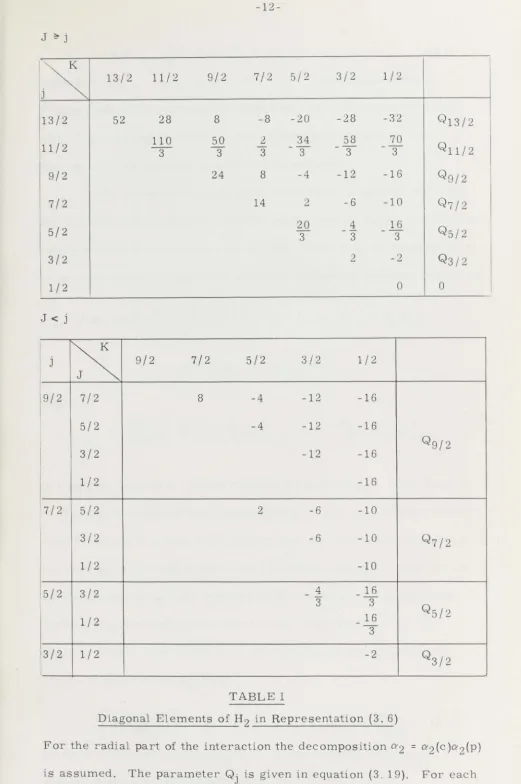
TABLE I

Diagonal Elements of H2 in Representation (3.6)

For the radial part of the interaction the decomposition 0'2

= O'2

(c)O'2(P)

is assumed. The parameter Qj is given in equation (3. 19). For each

K only values of J = K, K+l, .. . .. are admissible. We find ~

[image:23.561.23.544.15.799.2]

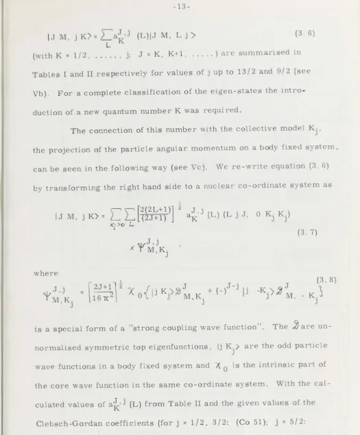
-13-\J M, j

Ki

=

La~,j

(L)/J M, L j>

L,

(3. 6)

(wIth K = 1/2, . . . , j; J = K, K+1 , . .. .. ) are summarised in

Tables I and II respectively for values of j up to 13/2 and 9/2 (see

Vb). For a complete classification of the eigen-states the

intro-duction of a new quantum number K was required.

The connection of this number with _{the collective model K j},

the projection of the particle angular momentum on a body fixed system,

can be seen in the following way (see Vc). We re-write equation (3. 6)

by transforming the right hand side to a nuclear co-ordinate system as

where

(3. 8)

K.)

J

is a special form of a "strong coupling wave function". The:J are

un-normalised symmetric top eigenfunctions , Ij K.> are the odd particle J

wave functions in a body fixed system and )( 0 is the intrinsic part of the core wave function in the same co-ordinate system. With the

cal-culated values of

a~'

j (L) from Table II and the given values of the

Clebsch-Gordan coefficients (for j = 1/2,3/2: (Co 51); j = 5/2: (Sa 55); j = 7/2, 9/2withL~4: (Si 54)), we obtain for a proper

choice of phase of the

a~'

j (L)

1

> '

[2(2L+1

n

'2

L' (2J+1)J aK J

,j (L) (L j J; 0 K· K.) =

J J

('

°KK.

J

So we see that our eigenfunctions (3. 6) are identical with the

strong coupling wave functions (3. 8)

(3. 9)

[image:24.556.13.539.16.651.2]

~

J - ~ J - ~ 3

j J +

-2 2 2

\:: eli

1 1 + 1 >

eli

2" 2" _"

.~

I ....,

3 3 _-

~

_{[ 3 (2J+3)}

_J

_t

_~

[(2J-1)]t

~ 2" 2 (2J+2) 2 (2J+2) -a -a

0

"

_

~

[ (2J -1) ] t

1 .~ I

1

_.!.

_{[3 (2J + 3) 12} ....,

2" 2 (2J+2) 2 (2J+2) •

1 1 1

5 5

.!. [

(2J+5)(2J+3) ] 2 1 [10 (2J+5)(2J -3) ] 2 1 [5 (2J - 1 )( 2J -3)] 2 ~ 2" 4 (2J)(2J-2) 4 (2J+2)(2J -2) 4 (2J+2)(2J)

t::

eli

>

1

[ (2J - 7)2

1

t

1 eli

3 ~ _{[ 5 (2J+3)(2J-3)}

J

₂ 1 _ ~ [ (2J+5)(2J -1)

1

2

"

2" 4 (2J)(2J-2) 4" 2 (2J+2)(2J -2) 4 (2J+2)(2J). .~

I

....,

1

_

3.

[(2J+3)(2J-1)] t

~

l

(2J+5)(2J+3)] t

1 _{~ [10 (2,J-1)(2J-3)r}

2" 4 (2J)(2J -2) 4 (2J+2)(2J-2) - 4 2 (2J+2)(2J)

~

J-~

2 J+.!. 2 J+~ 2

1 -a

1 -a

~ 2 - 1 0

"

.~

I

! [ (2J+~)

1

t

...., 1

3 3 _{1 [ (2J-1)] 2} \::

2:

2" 2 (2J)_ 2" 3 (2J) eli

>

eli " .~

1

~

_{( 3 (2J - 1)}

1

_t

_{.!. [(2J+3)]}

_t

I

2" 2 (2J) _ - 2 (2J) ....,

1 1

_1

[(2J-3)(2J-1)] t

~

5 _{1 [ (2J+5)(2J+3) )} 2 1 ( (2J+5)(2J -3)] 2

2" 4 .5 (2J+2)(2J) -4" 10 (2J+4)(2J) 4 (2J+4)(2J+2)

-a

-a 0

1(2J+3)(2J-3)

J

1

1 [ (2J+9)2 ]

t

~

( (2J+5)(2J-1)r

"

3 3 '2 .~

2" - 4" . (2J+2)(2J) + 4" 2 (2J+4)(2J) - 4 5 (2J+4)(2J+2>, I ....,

1

_

_~

(2

_{(2J-3)(2J-1)]} '2 1

_3.

_{[(2J+3)(2J-1)] t 1 [ (2J+5)(2J+3)J2} 1 2" 4 (2J+2)(2J) + 4 (2J+4)(2J) - 4" 10 (2J+4)(2J+2)

TABLE II

Expansion coefficients

a~'

j (L).

t--3 p.l u _.-.

ro

"'""

"'"" ...-. () o ~ r+

j

=

7/2

J - j

=

even

~

J - 7/2

1.

₁

U

_{2J +}

n (

_{2J + H (}

_2J

_{+ r l] t}

2

8

{2J 2J-2

2J-4

j

1[7{2J+H {2J+r~

_(2J-fl}

_t

2

8

{2J 2J-2 2J-4 _

1

_{1[ 21 (2J + J) (2J}

-1

_{Z (}

_{2J -}

5

II

_t

2

8

(2J) (2J-2

2J-4

.

1

1[35(2J-1~(2J-r~(2J-~l]

_t

2

8

(2J) 2J-2

2J-4

- -

-J - j

=

odd

~

J - 5/2

1.

_

1[7(2J+:Zl~2J+H(2J+rLl

t

2

8

(2J+2 {2J 2J-2

.2

_

j[(2J+2}~2J+N(2J-~l]t

2

8

{2J+2 {2J 2J-2

1

_

ll

_{3 (2J+ Jl}

~2J-r~ (2J-~lJ

_t

2

8

(2J+2 (2J 2J-2

1

_1[5{2J-1l~2J-N(2J-r)]t

2

8

(2J+2 (2J

2J-2

-J - 3/2

J

+ 1/2

1 [21 (2J +7 l

~

2J

+ H (2J- f

II

t

8

{2J +2 {2J 2J-4 _

1 [35 (

8

2J

{2J+4 (2J 2J-2

+ 7 l

~

2J

- r

~

( 2J -

~

l] t

1[

(2J+~~(6J-12)2

1t

8"

3 {2J+2--2JH2J-4)

,

-

8"

l [

5

-2J+4·-2J){2J-2)

~2J-JH2J+12l2

] t

1[

(2J-r

t(2J_2 2) 2 j t

'8

{2J+2--2J) {2J-4)

- 8"

1 [

15 {2J+4)-2J){2J-2) _

( 2J +

~

H

2J - 2 l 2

~

t

_ 1[

15(

2J

+J)

~ 2J-1~

(2J-r

lj

t

8

{2J +2 {2J) 2J-4

1 [( 2J + 2)

8

{2J+4 (2J 2J-2)

~

2J + r

~

( 2J -1 l] t

----~

J -

1/2

J + 3/2

_

1[35~2J+:Z~ ~2J+2~ ~2J-2~J

₈

_2J+4

_2J+2

_2J-2

t

_-

1[21(2J+:Z~~2J-Jl~2J-~ll~

₈

_{2J+

_{(2J+2 (2J}

1 [

(2J+~)

(2J-17l

2

'

1

t

-

8"

5{2J+4)-2J+2){2J-2)

1 [

8"

3

{2J+b--2J+2)-2J) _

(2J-1~(6J+2~}2

It

l[

(2J- Jl (2J+7)2

'

]

t

8"

1 5 {2J+4) (2J+2) {2J-2)

-

*

8

{2J+b--2J+2)-2J)

(2J+H(2J+1

t

}2 It

1[~2J+J~~2J-1~~2J-J~]t

₈

_2J+4

_2J+2

_2J-2

_

1[15(2J+2~~2J+Jl ~2J-ll]t

8

{2J+

{2J+2 (2J)

- - ~.

-J + 5/2

ll

₈

7{2J-

_{{2J+4 {2J+2 {2J}

l l

~2J-Jl ~2J-r}1

t

j [( 2J +:Z l ~ 2J- J

l

~ 2J-1

l1

t

-

8

{2J+4

{2J+2 {2J)

1 [3 ( 2J +7)

~

2J + 2}

~

2J -1

II

t

8

{2J+4 (2J+2

(2J)

1[5(2J+:Z)

~2J+2l ~2J+rl]t

-

8

(2J+4 (2J+2 (2J

- .

J + 7/2

_

1[~2J_1~~2J-J~~2J-2~]t

8

2J+b

2J+4 2J+2

1[7~2J+~~ ~2J-1~ ~2J-J~]t

₈

_2J+

_2J+4

_2J+2

_ 1 [21

₈

~2J +~~ ~

_2J+

2J +

_2J+4

2~ ~ 2J-1~

_2J+2

Jt

1-3 ~ r-' (t) H H

-

n

o ~

.

---~

~ '2 7 '2 5 '2 :\ 2" 1 2"

.I _ i!

2

~ [(2.T+:J)(2J+5)(2.)+7)(2J+g)

1

;

16 (2.1)(2J-2)(2.1-4)(2J-6)

. 1

2

1

(2J+7)(2.)+5)(2J+3)(2.1-7)J 2

16 (2J)(2J-2)(2.J-4)(2J-6)

1

~

l

(2J+5)(2.1+3)(2J-5)(2,)-7)] 2

16 (2J)(2.1-2)(2J-4)(2J-6)

1 2 [21(2J-7)(2.)-5)(2J-:1)(2J+3)'1 2 16 (2J)(2.! -2)(2J -4 )(2.) -6) ,

2

i

H(2J-l)(2.J-3)(2J-5)(2J-7)] ;

16 (2J)(2.1-2)(2J-4)(2J-6)

J -J odd

r:;:

7

J -l'

q -=2 _{[(2J+9)(2.)+7)(lJ+5)(23+3)] l} '2 16 (2J+2)(2.))(2J-2)(2J-4)

1

7 _ 2.. [(2J+7)(Z.J+5)(2J+l)(2.J-7)

I

2 '2 16 (2J+2)(2.1)(2J-2)(2J-4).

1 '; -.!..Q

r

12J + 5 )(2.)'3)(2J-5)(2.1-7)]' 1 16 . (2.J+2)(2.J)(Z.I-2)(1.J-4) .

3 ~

r

21(2.1+3)(2J-3)(2.)-5)(2J-7)]1

2 16, (2.J+2)(lJ)(2.1-2)(2.)-4)

~ 114(2.1 -1 )(2J -1)(2.1 - 5)(2J -7)]1

1

2 16 (2J '2)(2J)(2.J -2)(2.1 -4)

.I - %

~ 1 (2.J+5)(2J+7)(2J+9)(2J -7)

I

I

16 (2J+2)(2J)(2J-2)(2J-6)_

2 [(2J+7)(2J+5)(10.)-39)21 1 16 (2J+2)(2J )(2J -2)(2J -6),

4 (2H5)(2J-5)(4J-Zl)"

)

r

2

161 (2J+2)(2J)(2J -2)(2J -6)

1

12 [21 (2J-5) (2.)-3) . 2

-16 (2J+2)(2J)(2J -2)(2J - 6)

1

_2. [14 (2J+3)(2J-l)(2J-3)(2J-5)] i 16 (2J+2)(2J)(Z.1 -2)(2J -6)

J -~

2

~ [21(2J+D)(2J+7)(2JI_{5)(2J-7)1 ;}

16 (2J+4)(2J+2)(2J)(2J-4),

? ] 1 -2 [21(2J+5) (2J-7) (2.1-11)" 2

16 (2J+4)(2J+2)(2J)(2J-4)

20 121 (2H5) (2J -5)

1

i 16 ,(2J+4)(2J+2)(2.1)(2J-4)

4

I

(2J-3)(2J-5)(4.J+13)2

1

;

16 (2.J+4)(2J+2)(2J)(2J-4)

2 \6(2J+3)(2J-l)(2.1-3)(2J-5)1 )

16 (2J+4)(2J+2)(2J)(2J-4)_

J -.!. J + ~

2 2

~ [14(2J+9)(2J+7)(2J-5)(2J-7)J i 16 (2JH)(2J+2)(2J-2)(2J-4)

2 [21(2J+Q)(2J 3)(2J-5)(2J-7)1 1

16 (lJ+6)(2J+2)(2J)(2J-2).

1 [14(2J+7)(2J-5)(2J-31)2 11 16 (2.1>4)(2J+2)(ZJ-2)(2J-4)

-2 [ 21(2J-3)(2J-S)(2J+l3)2 r

16 (2J+6)(2J+2)(2J)(2J-2)

-2 l14 (4J2 +12J - 67)2

1

;

16 (2J+4)(2.J+2)(2J -2)(2J -4),

20 [ 21 (2J+7) (2J-3)

J

i 16 (2J+6)(2J+2)(2J)(2J -2) _

-2 [6 (2J+5) (V-3)(2J-ll)2

1

}

16 (2h4)(2J+2)(2.!-2)(2J-4),

4 [(2J+7) (2J+5) (4J-9)2

-

I

i

16 (2.1+6)(2J'2)(2J)(2J-2).

~ [ (2J+5)(2J+3)(2J-3)(2J-l)] ~ 16 (2J+4)(2J+2)(2J-2)(2J-4)

~ [6(2J+7)(2J+5)(2J+3)(2J-l)] l 16 (2J+6)(2J+2)(2J)(2J-2)

J+.!. J + 5

2 'Z

-=2

r

I4 (2J+9)(2J+7)(2J-5)(2J-7)'\; 16 (2J+6)(23+4)(2J)(2J-2),

.:.2 [(2J+9)(2J-3)(2J-5)(2J-7)] l

16 (2J+8)(2J+4)(2J+2)(2J)

~ [14(2J+7)(2J-5)(2J+33)2Ii

16 (2J+6)(2H4)(2J)(2J -2)

2

I

(2.J-3)(2J-5)(10J+49)2J ~ IT ,(2.1+8)(2J+4)(2J+2)(2J)

2 1 14 (432 - 4J - 75)2 ] l 16 (2J+6)(2H4 )(2J)(2J -2)

-4 [ (2.J+7)(2J-3)(4J~25)2'1 l 16 (2J+8)(2J 14)(2J+2)(2J)

-2 [6(2J+5)(2J-3)(2J+13)2 '\ ~

16 (2J+6)(2H4)(2J)(2J -2).

12

i

21 (2.1+7) (2J+5) ) t

li3 (2J+8)(2J+4)(2J+2)(2J)

.:.2 [(2J+5)(2J+3)(2J-l)(2J-3)] ;

, 1

2 [14(2J+7)(2J+5)(2J+3)(2J -1) J 2

16 (2HG)(2J+4)(2J)(2J-2) 16 (2J+8)(2J 14)(2J)(2J+2)

J+2

2

2 f(2J -1 )(2J -3)(2J -5)(2J -7)

1

i

16 i (2J+6)(2.1+4)(2J+2)(2J) .

1

:.2

i

(2J+Q)(2J -1 )(2J - 3)(2J - 5)

l

'

16 (JJ+6)(2.T+4)(2J+2)(2J)

1

.!..Q f(2J+9)(2J+7)(2J-l)(2J-3) \' 16 . (2J+6)(2J+4)(2J+2)(2J)

~ l21(2J+9)(2J+7)(2J+5)(2J-l)

1£

16 (2J+6)(2J+4)(2J+2)(2J)

~ (14(2J+9)(2J+7)(2.1+5)(2J+3)

1

;

16 (ZJ+6)(2J+4)(2J+2)(2J) •

J+~

2

~ [(2J-l)(2J-3)(2J-5)(2J-7)]l 16 (2J +8)(2J+6)(23+4)(2.1+2)

1

3

l

(2J+9)(2J-l)(2J-3)(2J-5) 'I i 16 (2J+8)(2J+6)(1J+4)(2J+2),

1 -6 [(2J+9)(2J+7)(2J-l)(2.1-3)] 2

16 (2J+8)(2J"6)(2J+4)(2J+2)

2 [21(2J+9)(2J+7)(2J+5)(2J-l) 1 ;

16 (2J+8)(2J+6)(2J+4)(2')+2)

.=2 [14(2J+9)(2J+7)(2J+5)(2J+3)

1

;

16 , (2J+8)(2J+6)(2J+4)(2J+2)

~

-17-and that the expansion coeffIcients

a~'

j 'L) can be glVen by the closed

expression

1

J ,j \2(2L+1)} 2

a K (L ) =

l

(2 J

+

1 ) (L j J; 0 K K) (3.11) As we have a sequence of J = K, K+1, . . . for each value of K and find that the eigenvalues of H2 are independent of J, we see tbat these

eigenvalues form the bases of various bands, the same as found in the

collective model. It is interesting to note that the degeneracy of the

wave function (3. 6) in K and - K is brought about automatically in the

procedure presented here.

Had we used a different core function

1

\ L , M

n )

=

X

r

2 L+ 1

\2

r»

L .0-

l

8 [2 M,D.

with L = D , .0+1, ... , we would have obtained

and

1

I

J M K +Q, j K:> =

l

-2J+11

2

'1/

\jK>~J

16 ~I' ~ 2 fvn M, K~S2

aJ,j (L) =

K,Q.

1

l

2(2L+1)-\2 (L j J; .Q K K +fl.) ,

(2J+1) _

(3.12)

(3.13)

(3. 14)

if we assume a relation similar to equation (3.9). In this case , there is no natural degeneracy in the K quantum number (- j

-=

K ~ j) and for each j the J -sequence of the different bands depends on the value of D. .

We will, however, not pursue this line any further.

The eigenfunctions of H2 in equation (3. 6) are eigenfunctions of any of the operators Hn (n = 4, 6, . . . ) . For a special choice of the co-ordinate system , we have (Ro 61, p. 59)

Hn oc Y _n, 0 (g, 0) , (3.15)

which follows from the invariance of the tensor contractions Hn under rotations. As the coupling rules for spherical harmonics

(Ro 61, p. 61 ) give

we find that if any eigenfunction diagonalises H 2, it WIll diagonalise H4

and subsequently H6 etc.

Using the general formulae developed in the theory of angular

momentum coupling, we can express the matrix elements of Hn in

representation (3.6) in the general closed form (see Vd):

(' L2n+1] t

(JM, jK\HnIJM, j'K')= _{0KK'L4 1t} (j'nj; KOK)

3. ] 7)

x:

<,mtr II antc) 1\ intr>< j /I Hn(p) 1\ j'

>

,

if we assume a to be of the form a (c a (p'. Besides the selectlon

n n ' n '

rule

6K = 0 (3. 18a)

we find

J' = j

+

n, . . . , Ij - n \

and (3. 18b)

l' = 1 + n, 1 + n-2, . . . ,

11

-

n

I

from the properties of the Clebsch-Gordan coefficients and the

properties of the reduced particle matrix element

<J

\\Hn(p)!l j'> = ( j 1/2 1 1lHn (P)I j'1/2l'>

For n = 2 and j = J', equation (3. 17) agrees with the expression

with

Q

j =

~[~(2j

+

3)(2j}2){2j){2j-1)1t

<intr lIa 2 (c) II intr) I( j I_I

H 2{P)1I

J>

,

(3. 19)

which can be obtained by means of a table of differences from the

values given in Table I (see Vb).

If we write

(~)2

=

(D

2 +

(1/

2(LD

(3.20a)

=

(D

2 -

(])2

2(f:-

.

D

(3.20 )

we have in equation (3. 20a) the rotational part of the customary collective

-19-represents the rotation particle coupling RPC (Ke 56). We see that

RPC is included in our Hamiltonian, as we have

(3. 22)

The matrix elements of H = C(L)2 in representation (3.6)

c

-can be calculated with standard methods (see Vel· The results are <J, j KI Hc_l J, jl K» = C

&"1

(J(J+1) + j(j+1)

JJ

-2K2 + (_)J+j (j+1/2)(J+1/2)

d'

1 ) , (3.23)

K2

1

<'

J ,j K I Hc I J, j 1 K'

>

= -C

&

..

l

LJ(j+1) - K(K+1)1 2

JJI K'K+1 J

1

X [(J+K+1) (J -K)) 2 (3. 24a)

1 <'J, j KIHcl J, jl K '

>

= -C &jjl

6

K'K-1 U(j+l) - K(K-1)J 2

1

x[(J+K) (J-K+1)J 2 (3.24b)

with the selection rules

6.j = 0, L\l '" 0,

~K

= 0, t 1. (3. 25)

These expressions are in accord with the results obtained by a direct

calculation from the values of the

a~'

j (L) of Table II, which are

sum-marised in Tables III and IV for j <f 9/2.

The matrix elements of the remaining term of the Hamiltonian

(~.~) can be obtained with similar methods (see Vf)

1

<

J M , j K

I

(s. L) I J M, j 1 K 1

>

= ( [J (J + 1 )

J

2 (J 1 J; K 1 ~K K)

1

)( (jl 1 j; K ' 6K K) -

cl

_jj, 0KK' U(j+1)] 2

_(_)J-jl

(21-~(J+1/2)(j'

1 j; -1/211/2)

<j\l ~llj'> ' (3.26)

where 6K = K - 1(1 , with the selection rules

~j = 0, ~ 1, 6, 1

=

0, /:;,. K

=

0, ± 1 (3. 27)

TABLE III

K

9 7 5 3 1 _-1

-- -

-2 2 2 2 2 2

J -j = even J -j

=

odd

j

9 63 1 49 81 87 107

-

- -

-

-

- -5J + - 5J +

-2 4 4 4 4 4 4

7 35 13 45 53 _4J

_+~

-

- -

- 4J +

-2 4 4 4 4 4

5 15 17 27 39

- - -3J + - 3J +

-2 4 4 4 4

3 3 _{-2J +}

~

2J

+~

-

-2 - 4 4 4

1 1 3

2 -J -

"4

J + -4

Diagonal Matrix Elements of Hc/C in Representation (3.6). For convenience only the values T =

1..

(H - C J(J + 1)) are tabulated.

C

c

matrix element

< j II ~/I j '/' =

<

j 1/2 1 II ~ 1/ j' 1/2 l'

>

.

The last term on the right hand side of equation (3.26) stems from the

fact that for K

=

K'

=

1/2 a value of K+K' = 1 can occur.

If we employ equation (3. 20b), we can extract from (3.23) and

(3.24) the matrix elements of (~.

1).

As we have

and

<J, j

KI

(!::.i)IJ, j K'> =

L{a~

,

j

(L)

a~

"

j

(L) (_)L+j-J L

1

W(LjLj;Jl) [(2L+1)(2j+l)] 2 <LIi!:-IIL>} <jIl1Uj>

we can relate the matrix elements of (~.!:-) and(!:-

.1)

for the case

6.j = 0 by

< \

C~.

'

L)I

>

= < j u

~

u j?

<

I (!:-.

1)

1

>.

~(j+l)J 2

In fact, equation (3.26) reduces to the matrix elements of

(3. 28a)

[image:31.546.15.533.15.718.2]

TABLE IV

~

22

2.2

.2.1

.1

1

2 2 2 2 2 2 2 2

.2.

_-

~[(2J+9)(2J-7)]!

_{- 2 [(2J+7) (2J-5)J}

_t

_-

~

_{[21(2J+5) (2J-3)J}

_t

_{- [6(2J+3) (2J-1>J}

_t

2

2

_-

~

_{[7(2J+7) (2J-5)1}

_t

_{_}

~(2'J+5) (2J-3~

_t

_{_}

~

_{[1 5(2J+3)}

(2J-1~

_t

2

.2

_{- ;}

~(2J+5)

_{(2J-J)] !}

_{- [2 (2J + J)( 2J -1)] !}

2

.1

_{- ;}

~(2J+J)

_{(2J-1)] !}

2

~ ~ - -- __ L- - - -.~-- - --- - -- --

1

<jv~~j)[j(j+1)] "2 (~.j) in this case.

The situation can be summed up in the following manner, cases

(a), (b), (c):

(a) We assume that both the single particle spacing and the spacing of

the different K-bands are large enough that both j and K are good

quantum numbers. The matrix elements of the Hamiltonian (2 r 17)

then take the form:

z..)-"I 1

\

; " 1-2n=1} "2

(J, j K\HIJ, j K) = _{_ 411..-}

-1"\.·4

(j n J, K 0 K)

x<intr/I D' (c) lIintr><j IIH (p)1I j ) + C(J{J+1) + j(j+1)

n n

_2K 2 + (_)J+j (j+1/2) (J+1/2)

f

1 ) + D'(2(K2 - J{j+1)) K"2

J j r <JIi _l2.lI_j>

+(-) -

(j+1/2)(J+1/2)QK~)

[2j(2j+2)1

~

+f

-¥(j-l/2)fOr l

~

+

¥

(.i+3/2) for I

= j-1/2

~

= j+ 1/2

+ E(j)

with K = 1/2, . . . , j and J = K, K + 1; . . . .

(3.30)

Equation (3.30) is illustrated for fictitious parameters in Figure 1,

for j = ~ . It is equivalent to the usual collective model descnption

of the spectrum of odd-A nuclei in terms of various-unperturbed

rotational bands.

We can re-write the Hc and (~.~) parts of the total Hamiltonian

<

J, j K I Hc

+

D I (~. ~) \ J, j K> =

with

C(J(J+1) _ j(j+1) + 2(j(j+1) _ K2)

..!....(_...!..)_~_-J_

.

_

(j + 1/2)

+a(_)J+~

(J+1/2)~

1

K"2

. 1. {D'<jISIIJ· »

a = (-)J -2 (j + 1/2) 1 - _ 1

C L2j(2j+2)] 2

a

(3.31)

(3.32)

The quantity "a" can be interpreted as the decoupling parameter.

-23-36 13/2

36 712

53 13/2

18 9/2

18 3/2

8 5/2

40 11/2 _{6 1/2}

/ 1

E(52 /2) I

29 9/2

20 7/2

13 5/2

8 3/2

5/2 3/2

45 13/2

32 1112

21 912

12 7/2

5 5/2

~ E ( 5/2 _{,5/2 )}

FIGURE 1

Illustration of equation (3.30) for the case j = 5/2 with fictitious

parameters. The quantities E (j, K) represent the J -independent

part of the Hamiltonian. The integers I indicated on the left side

of each band represent the rotational (core) part: Hc -= I C. The

degeneracy in the rotational part of the K =

t

band for J = 3/2, 9/2;

[image:34.546.7.530.12.693.2]

spectrum in the case K = 1/2 arises from the partial decoupling of

the intrinsic motion from the rotational motion. The decoupling

parameter in this model has the form (Mo 57, p. 487)

a =

L

(-)j - tic. I 2 (j + 1/2) .

. J

J

In algebraic language, it stems from the fact, that for a strong

coupling wave function of the form (3.8) , the term (~.j) of equation

(3. 20a) gives cross contributions from the components with K. and

J

-K. in the case of K . = 1/2, as both J and j are vectors. As we have

J J

-to sum over all the particle states involved (I Cj \ 2 are the respective

amplitudes), this term depends essentially on the intrinsic motion.

In our case we have only one particle outside the core. The

de-coupling term arises from the properties of both the (~.!::) and (~.

1)

parts of the total Hamiltonian, but no summation is involved. Besides

the actual decoupling term

(_)J+t (J + 1/2)

6

1

K-z

the position of the bands is affected by the "decoupling parameter "

in this case.

For D' = 0, we obtain a decoupling parameter

a = (_)j-t (j

+

1/2) ,

which corresponds to the collective model term for one particle.

This would produce a spectrum degenerate in J = L

+

1/2 and L - 1/2

in the case of j = 1/2.

With the expressions for the matrix elements of s

1

<

j 1 / 2 l /I ~ II j 1 / 2 1

>

=

l.l2

₂ j _2j +

2]-Z

for 1 = j - 1/2

(3. 33) 1

r

2j

1

1.

=-

'2

.2j

+

2 . 2 for 1 = j

+

1/2

-25-a

=

(_)j-t (2j+1) (4jC-D') for 1 = J-1/2

4C(2j)

(3. 34)

=

(_)j-t (2j+1) ((4j+4) C+D') for 1 = j+1/2

4C (2j+2)

The signs of "a" for all possible combinations are given in

Table V.

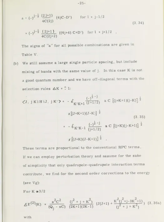
(b) We still assume a large single particle spacing, but include

mixing of bands with the same value of j. In this case K is not

a good quantum number and we have off-diagonal terms with the

selection rules 6K = ~ 1:

1 .

2" -J

<

J, j K \ H \ J, j K' '/ = -

J

~J

~

1/2)

K'K+1

1

a C [(j+K+1)(j-K)] 2"

1 )( [( J + K + 1) (J -K)] 2"

(3.35)

=

1 .

&

(_)2 -J

K'K-1 (j+1/2)

1

a C [(j+K)(j-K+1)] 2

X [(J+K)(J-K+1)] t

These terms are proportional to the conventional RPC terms.

If we can employ perturbation theory and assume for the sake

of simplicity that only quadrupole-quadrupole interaction terms

contribute, we find for the second order corrections to the energy

(see Vg):

ForK~3/2

2 2 .2 2 2 2 2

~E(2)(K)

= s C (J + j + K) (J(J+1) + K (j +j-3K +1)) (3.36a)

(Qj _ sC) (2K+1)(2K-1) (j2 + j + K2)

with

s - (

)t -

j 2a

(2j+1)

For K = 1/2

6E(2) (1/2)

(3.36b)

(j 2 + j _ 3/4) (J (J + 1) - 3/4) . (3. 37) 4(Qj - sC)

These results can be interpreted as a shift in the position of the

[image:36.546.6.530.17.729.2]

a/I a,

1

₌

j

-

2 1 1

₌

j + 2 1

D'

>

4jC - +

D'

=

4jC 0 + _J

-

2 1

=

even

D':;.O D'

<

4jC + +

C >0 D' ). 4jC +

-D'

=

4jC 0

-

j - _"2 1

=

odd

D'

<

4jC -

-D'

>

(4j+4)C +

-D'<O D'

₌

(4j+4 )C + 0 j

-

2 1

=

even

C >0 D' ( (4j+4)C + +

D'> (4j+4)C - +

D' = (4j+4 )C

-

0 _J

-

1

= odd

2

D'«(4j+4)C -

-TABLE V

[image:37.558.16.537.15.764.2]

-27-.6E(j,K) (3. 38)

and a change of the actual rotational part of the spectrum

C(J(J +1)) to C' (j, K)(J(J+1)) with

s 2 C (j2+j +K2)

C'(j,K) :: C(1 + ) (K:/: 1/2)

(Qr sC ) (2K+1) (2K-1)

(3.39)

forK2:3/2

For K :: 1/2, equation (3. 37) can be interpreted as giving rise

to a shift of the position of the band wIth the magnitude

,6E(j,K:: 1/2) :: (j2 + j _ 3/4) (3.40)

and a change of the rotational part of the spectrum to

C'(j,K:: 1/2) (J(J+1)+ (_/+t a'(j,K = 1/2) (J+1/2)

~

1) (3.41)

K2'

with

S2 C(j2 + j - 3/4)

C'(j,K:: 1/2) :: C(1 - -- )

4(Qj - sC)

(3.42a)

and a new decoupling parameter

a' (j ,K :: 1 /2)

2 .2 . / -1

= a(1 _ s C(J + J - 3 4))

4(Qj - sC)

(3. 42b)

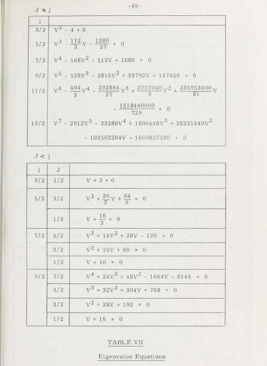
(c) Neither j nor K are good quantum numbers. In this case , we

have off -diagonal contributions from the 2n_ 2n pole forces with

the selection rules (3.18) and further contri.butions from the

term (~.~) with the selection rules (3.27) besides the RPC

terms discussed in Section b of this chapter. A detai led

exami.-nation becomes rather awkward, and it seems advisable to

employ the aid of an electronic computer for the diagonalisation.

The final eigenfunctions take the form:

\ '

\ J M"> ::

L,

c J (j, K)

I

J M, j K

> .

(3.43) j k

In the process of fitting the energy spectrum of an odd-A

nucleus the core parameter C can be taken from experiment.

estimate can mostly be obtained from the values of the

para-meters at the beginning and the end of the shell in questi on. The

parameters of Hn should be treated as free, although they can be

related for a fixed n, if the radial part of the different single

particle states

I

j mj) is given (e. g. , harmonic oscillator wave

functions) and a special form of the radial part of the

-2

9-IV Calculation of Static Moments and TranSItion Proba ill ties

The appropriate operator for electnc 2

A

-pole transitions

in the system even-even core and odd particle is

with the core part

Q (1\) (c) = e Z

R~

Y ') (j., ([) )

q c ~,q C IC

and the particle part

(~)

1\

Q (p) = e ff (~) r Y ~ q (j. ,

cp

)

q e P I ' , P P

while the operator for magnetic dipole trans~tlOns IS given by

(1 ) M

q

[ J

1 3 "2

4"i'G (g c q L

+

gil q

+

g s s q ) = J-L 0

ell

(!-L_o = = nuclear magneton).

2Mc

The quadrupole moment operator is then defined as

and the magnetic moment operator as

(4.1a)

(4. ib)

(4.1c)

(4. 2)

(4. 3a)

(4. 3b)

For the effective charge of the single particle e eff (A )

in equation (4. lc), we will consider the recoil effect of the core

on the particle ((Be 3 7), (Bo 53), (BW 52, p. 640)) in the combined

system

= e(l

+

(-l'

Z

PI'

A

Z

= (-) - e Af..

for a proton

for a neutron.

The correction to the ordinary charges e and 0 for proton and

(4.4)

neutron can be safely neglected for ~

>

2, especially as the single

particle part will be small compared to the core contribution for

even

A

,

if the core shows any collective structure.

We will not use the quadrupole corrections for the

distor-tion of the closed core shells by a non-spherical field of the outside

particles (Mo 58), as this would be inconsistent with the spherical

picture suggested in Chapter I.

The gyromagnetic factor of the core g _c takes the value

z

I

A for a uniformly charged nucleus, while gs and gl are the

con-ventional single particle values (BW 52, p. 31).

gs = 5. 587 for a proton

= -3.827 for a neutron

(4. 5)

gl 1. 000 for a proton

= O. 000 for a neutron.

The matrix elements of the operators (4. 1a), (4.2), (4.3a)

and (4. 3b) in representation (3.43) can be evaluated by standard

methods for the calculation of matrix elements of tensor operators

in coupled systems as given, e. g. , by Rose (Ro 61).

Case (a) E ~ - transitions

The partial lifetime

L

(E

1\)

of an excited state 1S related

to the transi tion probability T (E~ ) and the reduced transition

probability B(E~) by (El 57, p. 256):

-1

L(E;\)

=

T(EA)

=

8'i'C(1\ + 1) (_0 ) Ell 2~+1 hf1.((2f1+ 1)

~

~)2

hc

(4. 6)

'X.e2B(E~

;

J

~J'),

where E! is the energy difference of the transition and the

reduced transition probability is given by

e 2 B (E i\; J

-~

J') =

L

1

(J M \ Q

(~

)

I

J' M'

>,

2

M'''''l~M q

(4. 7)

The sum is to be extended over all possible values of the

angular momentum projection quantum number of the final

state M' and of q to give a fixed value of M. If we apply the

Wigner-Eckart theorem (Ro 61, p. 85) and the orthonormality

properties of the Clebsch-Gordan coefficients (Ro 61, p. 32ff),

-31-~I 2

~

I

(J 'A J, M' q lVI)

<

J 1\ Q

(~

) II J '

>

I

",1-tOJaM

= I(JIIQ(rI)IlJ') \ 2 (4. 8a)

2J' + 1 (A) 2

=( )1<J'IiQ IJJ)I

2J + 1

(4. 8b)

The last equation follows from the prInc.iple of detailed balance.

The matrix elements involved m equation (4. 8a) for the

core and particle parts with respect to representation (3.43)

can be calculated to be (see Vh)

1

( f\) \ ' J J'

[2i\+

1]

"2

(JIIQ (c)hJ')=eL..,c (j,K)c (J,K) 4

j k It...

x(J ~J'; K 0 K) Q((\) , (4. 9a)

where

Q( (\) =

<

intrll

ZR~

II

intr

>

(4. 9b)

is the radial part of the matrix element over the intrinsic

core wave function, and

)«((j',A,j; K'6K K) (J'AJ; K' bK K) (4. lOa)

J'-J I

+ (-) (j'tlj; -K' K+K' K) (J'~J; -K' K+K' K)) Q(A; j,j')

with the reduced matrix element

Q(rL j,j') =(j

1/211Ir;y~(p)/Ij'1

/2l

'>

1

= (_)II+j'+t -1-1 1(211+1)

(2j'+1)(2{\~ln"2

~

411.

J

J({l'Al ; 00 O)W(l'lj'j;{\ t)<1Iir;1I1 '

">

(4. lOb)

The selection rules are the customary

J =JI + ~, .. . .. , \JI

-111

for both the cases (4. 9a) and (4. lOa) and we have contributions

in the respective sums from states with

~K = O, .6j = 0, Al = 0 for the core part (4. 9c)

and j=jl+~ ,

1=1'+(1 , (4. 1 Oc)

.6K = 0,

±

1, . . . , ±~ for the particle part.

Furthermore we find that the core part gives only contributions

for transitions with even

A

(core states L = 0, 2, ... ), while

the particle part gives contributions for even f\, if both 1 and l'

are even or odd, and for odd (1 if the 1 and l' states are of

opposite parity.

In the case of the particle part of the transitio.n matrix

element, we find additional contributions for states with K and

K' such as to give K

+

K' = 1, . . . .. , ~ , which arise in a

simi.-lar fashion as the decoupling term in the calculation of the

Hamiltonian.

For the calculation of the matrix elements (4. ga) and

(4. lOa) of a specified odd-A nucleus only the parameters Q(~)

and

<

1 II r p 11'

>,

the radial part of the single particle

tran-sition, are required, once the expansion coefficients cJ (j, K)

are calculated from the fit of the energy spectrum. The

quantities Q((\) can (at least in principle) be extracted from

the various transitions between the core states, as

= (2(\+1) (2L'+1) (L'? L; 0 0 0)2 Q((\)2 e 2 4'iL(2L+1)

and so according to equation (4.6)

Q = + r(2L+l)

t((2(\+1)~

~)2

AT(E(\; L 4 L')

h

c

2

A+l]

~

(

~

) - U

2 L ,+ 1) 2 (

~

+ 1) (2/\ + 1) e 2 (L

'A

L; 0 0 0) 2 (

E;

. (

4. 11)

The sign of Q(?t) can be determined by the requirements for

the sign of the groundstate quadrupole moment of the odd-A

nucleus. The radial part of the single particle matrix element

could be evaluated in terms of a given single particle

wave-function.

The question of how far the core is polarised by the addition

of an outside particle can be examined most sensitively by the