A numerical approach to compensate for phase field interface effects in alloy solidification

Contents lists available atScienceDirect

Computational Materials Science

journal homepage:www.elsevier.com/locate/commatsci

A numerical approach to compensate for phase

fi

eld interface e

ff

ects in alloy

solidi

fi

cation

P.C. Bollada

, P.K. Jimack, A.M. Mullis

University of Leeds, United Kingdom

A R T I C L E I N F O

Keywords: Crystal formation Phasefield Alloy solidification

Non-equilibrium thermodynamics Anti-trapping

Solute trapping

A B S T R A C T

The use of a phasefield approach to simulate solidification of metallic alloys has many computational ad-vantages, but if obtaining quantitative results relies on the interface between phases being physically realistic, the computational advantage is much reduced. We propose here a method for compensating for a computa-tionally convenient large interface width by simply transferring a numerically derived 1D steady state anti-trapping current to a general non-steady 2D simulation. The method proposed is not restricted to dilute or ideal materials and has a high degree of interface width independence, illustrated here with two models, illustrating a broad applicability for the approach.

1. Introduction

In phase-field modelling of alloy solidification, applying the varia-tional principle to the Gibbs free energy results in equations for phase, solute and temperature, which optimally minimise the Gibbs free en-ergy, see[1]. The principle is clear and elegant but suffers from the practical disadvantage that the length scale of the solid liquid boundary is far smaller than that associated with solute and temperature diff u-sion. Consequently, phasefield modellers of solidification seek to use a larger than physical interface width to make the mathematical system computationally easier to solve. Simple adoption of a larger interface width, though, reveals that solutions are width dependent, see for ex-ample[2]. It is generally accepted that the approach to compensate for this is not to be found in a variational formulation, see[3,4](though, see the discussion inAppendix C which postulates a variational for-mulation for including anti-trapping currents). Rather, in an approach initiated by[3], one provides an extra degree of freedom at the level of the partial differential equations post variation by typically matching the phasefield equations model to a sharp interface model so that the resulting equations have an element of interface width independence. One feature of the application of matched asymptotic analysis to a sharp interface, e.g.[4,5], is that there is necessarily a degree of ap-proximation used in order to simplify the free energy functional to a point where analysis and comparison with sharp interface models be-comes tractable. For example, [6]extends[3,4]to use in multiphase models, but only for the simplest thermodynamics. It is of note that models that use physically realistic free energies for complex materials avoid this approach, e.g.[2,7].

The phasefield technique for alloy solidification, as established in simpler form by[8](WBM) is challenged by two phase modelling as described in[9]. This approach associates a unique concentrationfield, cLorcS, for the liquid or solid phases respectively, and the true con-centrationfield is constructed as a weighted average using the phase

field. The quantitiescLandcSare determined through a concentration equation and, crucially, a constraint. The constraint can take the form of proportionality, using a partition coefficient, or by equating the chemical potential. The latter led[10]to unify the methodology using a grand-potential functional (GPF) in place of the usual free energy. This served also to show that the two phase approach was equivalent to a variational formulation, in particular the equal chemical potential constraint in the two-phase formulation is a natural consequence of the new variational technique based on a GPF.

The GPF methodology has been applied in[11]to dilute alloys, but it is notable here that the GPF approach still requires an anti-trapping current to compensate for interface width, and thus, by implication, the model of[9]would benefit from an anti-trapping current to alleviate interface width dependence. [12]argues that the two phase models, with the constant chemical potential across the interface, needs mod-ification for rapid solidification, and suggest modifications that model this: namely, to replace the constant chemical potential constraint with equations forcLandcS. It is of note that[12]uses a physically realistic

=

δ 1.875nm in their 1D simulations (and so the method advocated in our paper naturally do not apply here). However, for 2D/3D simula-tions it is likely that larger interface widths will be computationally expedient and thus some method for compensating for artificial solute trapping will become necessary.

https://doi.org/10.1016/j.commatsci.2018.04.050

Received 13 March 2018; Received in revised form 19 April 2018; Accepted 20 April 2018

⁎_{Corresponding author.}

E-mail address:[email protected](P.C. Bollada).

Available online 25 May 2018

The GPF approach has also been extended to include non-dilute alloys in [13]. Here, central to the application of GPF is a quadratic approximation of the free energies about the equilibrium concentration values (in a multiphase setting),cijE. An approach which does not re-quire approximation to the data bases, for general alloy using an en-tropy functional is found in[14]. This latter approach is motivated by a general free boundary problem formulation and contains the equal diffusion chemical potentials of the two-phase method as a constraint. For more general thermodynamics the authors state that there is po-tentially a numerical bottle neck due to this constraint.

We choose to adopt and extend the method of[8]to allow quan-titative simulation of more general alloys, without recourse to special cases and approximations. It is of note that the application of the WBM approach to general free energy models has only previously been its extension to multiphase models. Consequently, this work represents a

first attempt at quantitative modelling, and modelling in itself, for so-lidification with arbitrary CALPHAD thermodynamics, whilst allowing a conveniently larger than physical interface width. In this sense the method may be seen as both an extension of[3,8], to allow rapid so-lidification modelling for arbitrary two phase binary alloys.

A constraint on the phasefield approach is that the interface must have sufficient resolution to capture thefinest curvature found at the solid-liquid boundary. But typically, tip radii,ρ≫d0∼1nm whered0 is the chemical capillary length, being the same order of magnitude as physical interface width, this being the distance over which long-range atomic ordering is lost at the interface between a crystal and its parent melt and which is typically a few atomic radii. Of more concern is the effect of large interface width on solute partitioning where the max-imum and minmax-imum values for solute concentration found at the solid-liquid interface are very much interface width dependent. This effect is known as artificial solute trapping, since it is a model dependent effect that tends to drive the partition coefficient closer to unity. Solute trapping also arises naturally in systems where the velocity of growth is sufficiently high, see[15], which analyses three regimes from low to high growth velocity. We propose here an approach which compensates for artificial (interface width induced) solute trapping, for realistically modelled binary alloys at arbitrary concentration.

In outline, the method we propose consists in solving a 1D steady state problem where the solution not only depends on input values for tip speed and tip interface width (and giventanhprofile), but also the strength of ananti-trappingcurrent, j. We seek the strength of jin the steady state 1D problem such that the maximum and minimum values for solute,c, within the interface, coincide with the equilibrium values found from the free energy functions for liquid and solid by well known common tangent construction. Oncejis found from the 1D problem we apply it to the full (non steady) 2D problem. New values for tip speed and width are extracted from the 2D simulation and used, inter-mittently, to solve the 1d problem, where the new value forjis applied thereon.

Wefind, for the PbSn alloy tested, and to a large extent model of [8], tested to make connection with a standard model, that this ap-proach gives a high degree of interface independence across a range of measures at the crystal tip. The measures used are tip radius, ρ, tip speed, V, and measures for solute partitioning: Δc≡cL−cS and

≡

k c cS/L, wherecSis the solid concentration near the tip andcLis the liquid concentration near the tip.

2. Solute trapping in 1D

In this section we focus on a specific phase-field model for alloy solidification, Pb-Sn in this case, in order to introduce the method proposed to compensate for solute trapping. This is based upon looking at the dependence of solute partitioning on interface width in a steady state 1D scenario.

The phase equations governing the evolution of phase,ϕ, (where

=

ϕ 0,1is solid and liquid respectively) and solute concentration,c, on a

domain,Ω, are, respectively (see, for example,[1])

= −

ϕ MδF

δϕ

̇ _,

(1) and

= ∇ ∇

c D δF

δc

̇ ·

(2) where

∫

= ∇

F f ϕ( , ϕ c, ) d ,x Ω

3

(3) Mis the mobility andD=[ϕDL+(1−ϕ D c) S] (1−c)/(RTvm), with the liquid and solid diffusivities DL≫DS, and R andvm the molar gas constant and the molar volume respectively. The free energy density,f, is decomposed into a surface part, f_S, and bulk partf_B:

= ∇ +

f f ϕ_S( , ϕ c, ) f_B( , )ϕ c (4)

where f_Bcombines, by interpolation, the liquid and solid free energy curves, illustrated inFig. 1for a simple constructed example. The sur-face term is

⎜ ⎟

= ⎛

⎝

∇ ∇ + − ⎞ ⎠

f W c( ) δ ϕ ϕ ϕ ϕ

8 · (1 )

S

2

2 2

(5) whereWis the surface energy of the barrier height between the two phases andδis a measure of the interface width.

In 1D and at equilibrium Eq.(1)becomes

= δF δϕ

0 S

(6) where

∫

=

FS _ΩfSdx ₍₇₎

The phase profile,1

Fig. 1.A constructed example free energy curves,

= − = − +

fL (c 0.25) ,2fS (c 0.75)2 0.1_{with the common tangent construction that}

give the equilibrium values ofcin the two phases:cSE=0.85,cLE=0.35.

1_{more generally the interface width, and even the general shape is modified by the}

bulk driving term. Some of our tests imply that the resulting profile is wellfitted by a continuous piecewise function using two tanh profiles defined on ϕ∈[0,0.5] and

∈

= + ⎛ ⎝

⎞ ⎠

ϕ x x

δ

( ) 1

2 1 2tanh

2 ,

(8) solves Eq.(6)in 1D, and has the property,ϕ x′( )|ϕ=1/2=1/δ (see

ap-pendixA). we adopt the double well potential in Eq.(5), in line with many authors, e.g.[8]in preference to, say, a quadratic potential (a double obstacle) to keep the equations smooth in the bulk:ϕ=0,1

The solute equation

= ∇ ∇

ċ ·D f_c, (9)

in 1D becomes

= ∂ ∂

ċ xD fx c, (10)

where we use the notation∂ ≡ ∂

∂ y x( ) x

y x x ( )

, and the functional derivative

≡∂

∂ f_c f

c. In a comoving coordinate system moving to the right at velo-city,u, Eq.(10)becomes

= ∂ D f∂ +uc

0 x( x c ). (11)

By writing

∂_{x c}f =f_{cc x}∂c+f_{cϕ x}∂ϕ ₍₁₂₎

one can solve forc x( ), once we knowϕ x( ). We assume, for this purpose, that the 2D phase profile normal to the boundary is well approximated by a tanh function, e.g. Eq.(8), but with a width,δ, ultimately extracted from a 2D simulation. Together with Eq.(12), an initial value forcin the solid, and a value for the tip speed,u, this allows us to solve Eq. (11).

To illustrate the effect of solute trapping we begin with two para-bolic example free energy curves for the liquid and solid phases in Fig. 1, where we can extract the equilibrium values forc_SE=0.85_and

=

cLE 0.35using the common tangent rule.

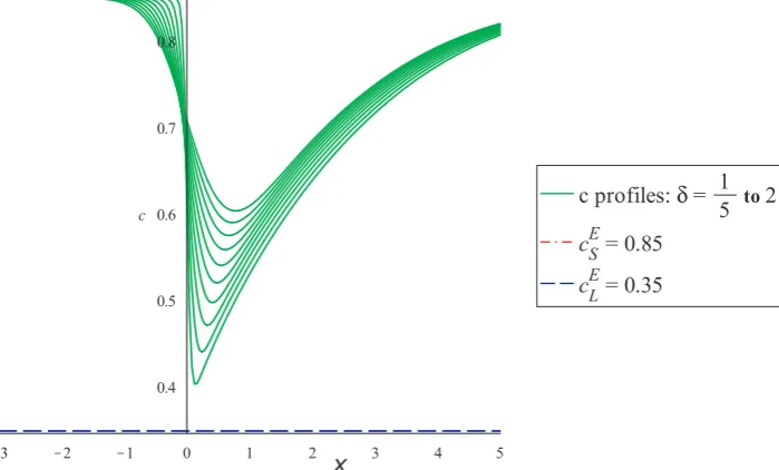
Using the solid value as a boundary condition, a selection of solu-tions are given inFig. 2for a different values of interface width,δ. Also superimposed in thefigure are horizontal lines presenting the equili-brium values for reference, where it is clear that even for the sharpest values chosen forδ, the peaks still do not reach the equilibrium liquid (minimum) value, and for progressively larger δ this minimum in-creases to get continually closer to the solid (boundary condition) value.

An approach to compensating for the interface width dependency in models with general thermodynamics can be found in[16]. It is based on the observation that including a regularising term in the free energy,

∇ ∇

δ2 c· c_{, to artificially increase the distance between the two extreme} values ofcshould compensate for the trapping effect. The main pro-blem with this approach is the introduction of 4th order derivatives into the solute equation, which[16]observe can have non-physical effects. On the other hand, a successful adoption of this approach, would result in a variational formulation, with consequent advantages (not least a reliable and thermodynamically consistent formulation of the tem-perature equation, see[1]).

We adopt a method more in common with the approach pioneered in[3]. To this end, returning to the full dimensional model, thefinal gradient term in Eq.(9)can be decomposed

∇f_c =f_cc∇ +c f_cϕ∇ϕ. ₍₁₃₎

We will show that compensation for the reduction of partitioning due to the large interface can be achieved by artificially modifying the second term,f_cϕ∇ϕ, to give

= ∇ ⎛ ⎝ ∇

∂ ∂ + ⎞⎠

c D f

c j

̇ ·

(14) wherej∝ ∇ϕ. The additional termjis known as ananti-trapping cur-rent.

Thefirst appearance of an anti-trapping current is found in[3], which compensates for interface effects in the dilute solution limit (linear solidus and liquidus lines, constantkE). Using our notation the current is defined by

= − ∇ ∇

aδ c ϕ ϕ ϕ

j Δ ̇

| |

0

(15) wherea=1/(2 2 ), andΔc0=|cLE−cSE|(where superscriptEindicates equilibrium values). The derivation of Eq. (15), along with the de-termination of relationships between other parameters in the dilute alloy formulation is firmly based on the analysis of sharp interface models for which the phasefield formulation is adapted to reproduce. Here, our starting point is the phase field formulation itself and its limiting behaviour as the interface width tends to zero. But rather than investigate this limit we aim to adapt the equations to make them nearly independent ofδin the range0<δκ<1(κis the tip curvature), whereδ is sufficiently small to resolve the curvature but as large as possible otherwise.

We integrate Eq.(11)from a point in the solid where it is assumed the gradients off_c vanish to give

Fig. 2.Example 1D steady state solutions to Eq.(18), for and free energies as inFig. 1, with various phasefield interface widths,δ=1, , ,2… 5

2

=D f∂ +u c c−

0 _{x c} ( _SE)

(16) which we rewrite as

=f ∂c+f ∂ϕ+ u −

D c c

0 _{cc x cϕ x} ( SE). ₍₁₇₎

On inspecting Fig. 2, we can find the local minimum value, cLm (or maximum depending on the convention forc), by solving

=f ∂ϕ+ u −

D c c

0 _{cϕ x} ( SE), ₍₁₈₎

with the phase profile

= +

ϕ x

δ 1

2 1 2tanh

2 .

(19) We note that Eq.(19)is only a solution of the equilibrium equation and that the dynamic profile is not atanhprofile, even with differentδ. That said, the dynamic profile with a given slope,1/∼δ at the interfaceϕ=0.5 is reasonably well approximated by Eq.(19), but withδreplaced by∼δ. The method we present uses a given tanh profile, but we take care to extract from the dynamic solution the actual interface width.

We seek to correctcLmto make it equal to the equilibrium value,cLE by introducing an extra degree of freedom,α, as follows:

= +α f ∂ϕ+ u −

D c c

0 (1 )_{cϕ x} ( SE). ₍₂₀₎

Wefind, in order to have a minimum,cLm, equal tocLE, that

+ = −

∂ =

α u c

Df ϕ

1 Δ

( _{cϕ x} )x x , 0

liq (21)

where, recall,Δc ≡|c_LE−c | SE

0 , andxliqis the unknown position where the minimum value in the liquid appears (n.b. if we knew xliq we could solve forαdirectly).

Assuming we have foundα, to apply the value of anti-trapping to the non-steady state 2D problem we take the tip velocity to be given by

= − ∇

u ϕ̇/| ϕ|and the jto be in the direction of the outward normal. Thus, in higher dimensions and non steady state, we write

= ∇ ∇ +

ċ ·(D f_c j) (22)

with

=αf ∇ϕ

j _cϕ . ₍₂₃₎

In practice, we require the anti-trapping to work for a range of values of δandu, so we search for a valueβsuch that there is a minimumc=cLE

in the solution of the ode, withα=βλ, i.e.

=f c x′ + +βλ f ϕ x′ + u −

D c c

0 _cc ( ) (1 )_cϕ ( ) ( SE) ₍₂₄₎

whereλis the non-dimensional parameter

=

λ uδ

DL, (25)

with u the tip speed, δ the actual interface width (such that

∇ϕ = = δ

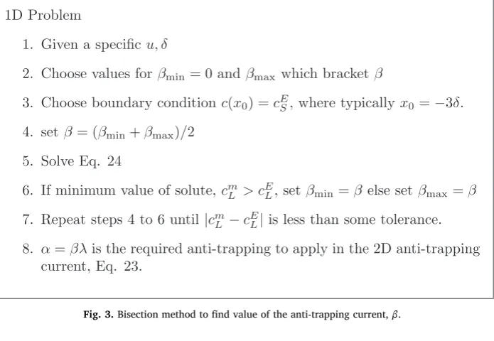
| |ϕ 1/2 1/ ) andDLthe value of diffusivity in the liquid. This allows us to havecLm≈cLEfor values from 0 toλ(in particular for speeds<u which will be found away from the tip). We summarize the procedure here inFig. 3.

We comment on the difference between Eqs.(21)and(24). In Eq. (21)we assume we know where the minimum is located,x=xliqand so

′ =

c x( liq) 0by definition. In Eq.(24)we solve and then search for the minimum (or maximum depending on convention) as per the table in Fig. 3. In short, Eq.(21)gives one solution for oneubut Eq.(24)gives a range of solutions, which is necessary sinceuvaries around the den-drite.

For our constructed parabolic free energy functions wefind a value ofβ=4.83compensates for interface width dependence in the steady state problem, with diffusivityDL=1,DS=0.001,u=0.2,δ=1. This is illustrated inFig. 4, where we not only see an exact compensation when

=

δ 1but also effective compensation for interface widths,1/5<δ<2. Since the interface width only varies slightly around a dendrite, this suggests that, ifu δ, are known approximately at the tip, then smaller values ofuat other locations on the dendrite surface will benefit from the same value of β (because of Eqs.(24) and (25) the current de-pendends linearly onuandδ).

In summary, the whole procedure is given inFig. 5and, when ap-plied to our constructed example free energy curves,Fig. 1, results in modified solute profiles given inFig. 4(to be compared to the no anti-trapping resultsFig. 2). The next section looks at the results of applying this procedure to a real complex alloy solution, e.g. Lead-Tin, and the WBM model of Copper Nickel, in single phase growth.

3. Results

This section contains results for a general binary alloy - Lead-Tin and also the simpler Copper-Nickel model of [8]. The anti-trapping method is seen to be effective in both cases, but appears more effective for the more complex model - PbSn.

Fig. 4.Solutions to the same steady state 1D problem as illustrated inFig. 2but with an anti-trapping current. The value forδ=1is chosen to be exact by the choice, =

β 4.83.

3.1. Lead-Tin simulation

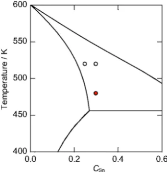
In this subsection we explore the effect of anti-trapping with PbSn across different parameters, with and without a thermalfield. In par-ticular we explore the single phase growth of the Lead-rich solid phase in the regions indicated in the PbSn phase diagram given in Fig. 6 generated using[17]. We explore the anti-trapping model in both iso-thermal and iso-thermal conditions. The single iso-thermal run being at 480 K andc=0.3. The complete details of the model and parameters are given in detail inAppendix Bwhere, for example, the units in the plots dis-cussed are detailed inTable 1.

We employ the numerical methods of [18] with a grid size of

=

x

Δ 0.39and domain size of800×800in units of the capillary length d0.

We inspect the results for the dynamic partition coefficient

=

k c cS/L; the normalised partition difference(cL−cS)/Δc0, whereΔc0is the difference in equilibrium values; tip radiusρ; and tip speedV. The latter two are in units ofL0=1nm andV0=0.2m/s respectively. We plot these quantities against the tip position, and thus these plots reveal the transient values. Steady state quantities may be extracted, in some cases, from thefinal tip position values if the plot has zero slope. Each sub plot contains three curves for each interface width, both with anti-trapping (AT) and without (NT) (6 plots in total). Broadly, the results without anti-trapping (NT) are interface width dependent and with AT are to a high degree width independent, even in some transient regions. In all the simulations, wefind that the AT current has an effect on the actual simulated interface width, i.e. AT tends to reduceδas compared to that without AT.

In the simulations we control the interface width with an input value δe which corresponds to the 1D equilibrium interface width, where the 1D solution is:

⎜ ⎟ = ⎡ ⎣ ⎢ + ⎛_⎝ ⎞_⎠⎤ ⎦ ⎥ ϕ x δ

1/2 1 tanh 2 .

e (28)

noting we define the equilibrium interface width

= ′ = δ ϕ x 1 ( ) . e

x 1/2 (29)

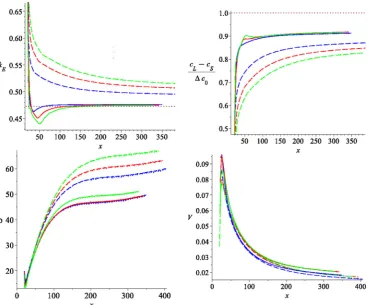
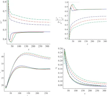
Fig. 7shows results of 6 simulations for three different interface widths (roughly in the range 5 to 10d0), with and without anti-trap-ping. Here the input values (in proportion to the 1D equilibrium in-terface width) areδe/ 8=4,6and 8 for blue, red and green respec-tively. These results demonstrate a high degree of interface width independence when AT is used, and, conversely, a δ dependence without AT. The two smaller interface widths display convergence for all quantities measured, but the highestδdisagrees slightly in the tip radius.

Fig. 8shows the equivalent set of results but with a change to the initial condition, c0=0.25, effectively making this a larger

under-cooling. In this case the input values are alsoδe/ 8 =4,6and 8 for blue, red and green respectively. Here the discrepancy between the AT results and the non-AT results is more marked, but still the agreement amongst the AT results is again very close: in particular there is agreement even in the tip radius for all widths.

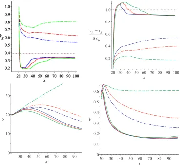
Fig. 9shows the equivalent set of results but with a change to the initial condition,c0=0.3,T=480K. For stability, the input values are reduced toδe/ 8 =3,4and 6 for blue, red and green respectively. Here the discrepancy between the AT results and the non-AT results becomes greater still, nevertheless the agreement within the AT results is very close. Even the largest interface widthδ=6.78approaches the steady state value of tip radius,ρ.

The thermal-solute phase field model, we employ, is detailed in AppendixB. This results in results given in,Fig. 10, we adjust the 1D solve to depend on tip velocity,V, the interface width at the tip,δ, and the temperature at the tip,Ti. The farfield temperature,T0, was set at 480 K and the tip temperature,Tiwas found to rise to503.7K. AtTi, the equilibrium values from the common tangent values forcare of course different to those associated withT0, and are the natural choice for the 1D solve, i.e. we useTinotT0to extract the AT current.

3.2. Simulations using WBM model

In order to explore the wider applicability of our technique towards interface width independence, and also to make connection with a simpler and well known model, we give results of simulations using the benchmark model found in[8]. This model, known as WBM, in fact, forms the basis for our model for PbSn, and by extension, any model using data base free energies in this way.

We use the model and parameters as described in[8, Table 1]with

Fig. 6.The phase diagram for Lead-Tin with white circle (520 K and =

c0 0.25,0.3) and red circle (480 K andc=0.3) being the regions of interest

explored in the simulations.

Table 1

Physical parameters used in the simulation.†these latent heat values are not used in the model which relies on the free energy- see text for detail.

Parameter Symbol Value

Char Length L0 10−9_m

Char speed V0 0.2m s−1

Diffusivity (Liquid) DL 10−9_m2_s−1

Diffusivity (Solid) DS 10−13_m2_s−1

Capillary length d0 10−9_m

Initial radius R0 20d0

Anisotropy ∊ 0.02

Surface Energy σA 0.033J m−2

Surface Energy σB 0.059J m−2

Melting Temperature (Pb) TA 600 K

Melting Temperature (Sn) TB 505 K

Operating temperature T 480,520 K

Initial concenteration c0 0.3, 0.25

Mol per unit Vol νm 54730 m−3

Interface width (Pb) δA 4,8,12×d0 Interface width (Pb) δB δA(T TB/ A)(σ σA/B)

Latent heat LA 2.61 8e J m−3_†

Latent heat LB 9.35 7e J m−3†

Kinetic (Pb) μA 0.0026/m K−1s−1

Kinetic (Sn) μB 0.0031/m K−1s−1

Mobility M (1−c M) A+cMB

Mobility (Pb) MA μATA

LAδA

72

Mobility (Sn) MB μBTB

LB δB

72 Barrier height W =WA(1−c)+W cB

Barrier height (Pb) WA _{T σ/(6 2L δ)}

A A A A

the exception of the kinetic parameters,

=

μ μ

[ _Ni, _Cu] [2.00,2.47]mK−1_s−1_{, which we found computationally} dif-ficult and so have reduced these by a factor of 100 toμ=[0.02,0.0247]. One feature of the model given in [8] is that the equilibrium con-centrations depend on the interface width,δ(via their expression for free energy Eqs.(8)to (10) and the expression for barrier height Eq. 36 in[8]). Hence, we chose a particular referenceδso that the equilibrium concentrations as given by[8]arecS=0.16and . This is in contrast to most other users of the model who restrict the model’s application to either dilute alloys, or where partitioning is negligible, e.g.[19].

Application of our method to WBM results inFig. 11, which illus-tratesΔcat all points around an early dendrite (whereΔc=cL−cS can be given as a function of angle,θ∈[0, /2]π , between a point on the 2D dendrite’s surface to the x-axis - see Fig. 12 for the corresponding dendrite shapes). In thefigure the dotted line indicatesΔc0, the equi-librium value. It is clear that there is convergence ofΔcacross a small range of input parameters, δe/ 8=4,6,8. The simulation was on a domain of800×800withΔx=0.39and so there are between 10 to 20 grid points across the interface.

The main feature ofFig. 11is the convergence, not just at the tip (θ=0, /2π ), but also to a high degree throughout the surface. The anti trapping current is computed from the tip speed and by design, a low speed reduces the current. Thus we expect good convergence at the tip and in between the dendrite arms (where the speed is much reduced). The agreement in between these extremes is due to a reasonable as-sumption that the amount of anti-trapping is in linear proportion to

speed. On the other hand there is not convergence when there is no anti-trapping-“NT”. The dashed curves inFig. 11make perfect sense in terms of the known deficiencies of the model. Growth is slowest atπ/4 so interface induced trapping is lowest and the solution is closest to equilibrium. Conversely, forθ=0, /2π velocity is at a maximum, so the largest departure from equilibrium is to be expected.

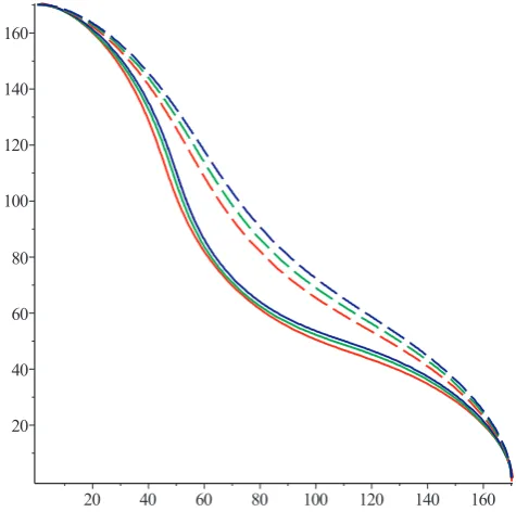
A plot of all the corresponding dendrites is given inFig. 12, all at the same tip position. Clearly there is better agreement with the anti-trapping model between the different interface values, which may be contrasted with the straight phasefield model (dashed lines). Thefigure adds weight to the assertion that even qualitatively, dendrite formation may well be incorrect without anti-trapping.

4. Discussion

The immediate observation from the above results is that compen-sating for solute trapping alone seems good enough to give results with a high degree of interface independence. Clearly, as is commonly ac-cepted and is the case here, the interface width must still be less that the tip radius. The rule of thumb being δ<ρ/2. Yet the 1D solve uses equilibrium values forcSE andcLE which differ significantly from the values found in the dynamic setting, as should be expected since there is natural solute trapping for higher velocities associated with increasing undercooling. The question that needs to be addressed is: why does the use of equilibrium values from the 1D steady state model give such satisfactory results in the dynamic setting where the dynamic partition

Fig. 7.Results for PbSn,c0=0.3,T=520K,δe/ 8=4,6,8(blue, red and green respectively). Clockwise from top left: dynamic partition coefficient,kE; concentration difference normalised with equilibrium valueΔ /Δc c0; tip speed,V; tip radius,ρ. The dashed results are without the anti-trapping and solid lines with anti-trapping. There is a high degree of interface independence for the latter across all measures. All dimensioned quantities are in units of length,L0=1nm and velocity,

=

values,cSandcLare (significantly) different from the equilibrium ones? An intuitive answer to this can be made by examining the case where the farfield (and initial condition) forc0is increased to a point where the undercooling is reduced to near equilibrium and the tip velocity becomes very small. In this scenario, the equilibrium values forcSEand c_LE_{are unchanged and are approached by the dynamic values, and the} only change for the 1D solve is the lower tip speed. The results above suggest that there is a near linear proportionality between tip speed,V, and the size of anti trapping in all the cases considered above. The Peclet number for these simulations is,Pe=ρV D/ L∼0.5. The predic-tion, therefore, is that the method might be less effective in situations with significantly higher Peclet numbers.

For smallV,[8]propose a model for the partition coefficient, in their notation

= − −

k kE(1 VM 1Γ )0 (30)

where, in our model, we write this withV∼≡2Vτ0/(3d0)

= − + ∼

k kE[1 V O V( )] 2

(31)

where τ0=1/MW and the capillary length

∫

∼ ≡

−∞ ∞

d0 (2/3)/Γ0 (2/3)/ ( ) dϕ_x2 x for an interface widthδ∼d0. Now, since the chosen characteristic time and lengths in our simulations are τ0andd0, we can read offthe non-dimensional number,∼V≡(2/3)Vτ d0/ 0 from the figures, the highest being from Fig. 9, where

≈ × ∼

∼

V 0.153 (2/3) 0.102. Thus indicating k∼0.898kE. Our result in Fig. 9, for the value for the smallestδ=4d0being:k k/ E=0.887, which is clearly very close to this linear prediction.

Finally, inAppendix Cwe seek to put the anti-trapping current into a thermodynamic context. This not only shows that the anti-trapping term can be put into a variational form, but also that the anti-trapping current is approximately entropy neutral. We then go on to make a connection with other work,[22], which postulates a cross term, re-lated to anti-trapping, in the phasefield equation.

5. Conclusion

We have presented a scheme to compensate for interface width dependence in general phase field modelling of metallic alloys. The scheme consists of a steady state 1D solve to extract an anti-trapping current,j, such that equilibrium partition values for solute are retained independent of the interface width. This value forjis then applied, to a general 2D simulation, with the modification that the anti-trapping is proportional to velocity and interface width (which vary along the dendrite surface). This straightforward approach is seen to be very ef-fective in the first unsteady problem chosen, across a range of tem-peratures and solute concentration, and also in the WBM benchmark problem.

Fig. 9.Results for PbSn at the highest undercooling,c0=0.3,T=480K,δe/ 8=3,4,6(blue, red green). Clockwise from top left: dynamic partition coefficient,kE; concentration difference normalised with equilibrium valueΔ /Δc c0; tip speed,V; tip radius,ρ. The dashed results are without the anti-trapping and solid lines with anti-trapping. There is a high degree of interface independence with AT for the latter across all measures, but without, the results disagrees significantly for different

Acknowledgements

This research was funded by EPSRC Innovative Manufacturing Research Hub in Liquid Metal Engineering (LiME), Grant No. EP/ N007638/1.

Fig. 10.Results for PbSn at the highest undercooling,c0=0.3,T=480K, with a thermalfield. Clockwise from top left: dynamic partition coefficient,kE; con-centration difference normalised with equilibrium valueΔ /Δc c0; tip speed,V; tip radius,ρ. The dashed results are without the trapping and solid lines with anti-trapping. There is a high degree of interface independence with AT for the latter across all measures, but without, the results diverge significantly for differentδe. All dimensioned quantities are in units of length,L0=1nm and velocity,V0=0.2m/s as given inTable 1.

Fig. 11.Plot ofΔcagainst the angle subtended between the x-axis and a point on the dendrite surface. The dotted line represents equilibriumΔc0. The lowest velocity is found atπ/4and the highest being at the tip -θ=0, /2π . The effect of interface width onΔc is much more noticeable without anti-trapping for all

∈

θ [0, /2]π . Fig. 12.A plot of the corresponding dendrites (using the same color code as

Appendix A. Equilibrium 1D solution to the phasefield equations

Beginning with the 1D equilibrium functional equation, Eq.(6),

∫

ϕ ϕ ϕ ϕ x

8 · (1 ) d 0

S Ω

2

2 2

(32) is follows, by applying the variation derivative, that

∇ = − −

δ

ϕ ϕ ϕ ϕ

8 2 ( 1)(2 1)

2 2

(33) which, upon substitution, is satisfied by Eq.(8)as required.

Appendix B. Model detail and parameters

One of the simulations had a dynamic temperaturefield for which we used the model detailed in[1]

= ∇ ∇ −⎛ ⎝ − ∂ ∂ ⎞ ⎠ ∂ ∂

C T κ T T

T f ϕϕ

̇ · 1 ̇

p

(34)

where ≡ − ∂ =

∂

Cp T ,κ 100D f

T L

2

2 . The other parameters and functions used in the PbSn model are given below in the tables: In Table 1, indicated by †_{, the latent heat values are evaluated using ≡ − −} ∂

∂ E ϕ c T( , , ) (1 T )

T δF

δϕ with LA=Δ |EPb≡E(1,0,TA)−E(0,0,TA) and

= ≡ −

LB Δ |ESn E(1,1,TB) E(0,1,TB), whereϕ=1(0)is liquid(solid), andc=0(1)is Pb(Sn).

The bulk free energy is given by interpolating between solid and liquid free energies using the monotonic function,g=ϕ2(3 2 )− ϕ_{, to give}

∑

∑

∑

∑

∑

∑

f g ϕ f c T g ϕ f c T S c T

S RT c c c c

f c g T cg T f c T

f c g T cg T f c T

g h T T g h T T

g h T T g h T T

f f Tf c c f f Tf c c

( ) ( , ) (1 ) ( , ) ( , ),

[ ln (1 )ln((1 )],

(1 ) ( ) ( ) ( , ),

(1 ) ( ) ( ) ( , ),

( ), ( ),

( ), ( ),

( ) ( ), ( ) ( ).

B L S M

M L A L B L RK L S A S B S RK S A L i

AL i i _BL i

BL i i

A S

i

AS i i B S

i BS i i

RK L

i

L i L i

i RK

S

i

S i S i i 1 8 , 1 8 , 1 8 , 1 8 , 1 2 1 , 2 , 1 2 1 , 2 , (35) These functions are the standard way CALPHAD methodology,[20], represents solute-thermal dependence. Heref_RKindicates Redlich-Kister model; SMindicates the entropy of mixing; and the pure thermal dependence is given by Gibbs vector constants and functions in the following array:

i _h

AL i, hBL i, hS iA, hBS i, T Ti( )

1 −2977.961 1247.957 −7650.085 −345.135 1

2 93.949561 51.355548 101.700244 56.983315 T

3 −24.5242231 −15.961 −24.5242231 −15.961 Tln( )T

4 −0.365895e−2 −0.188702e−1 −0.365895e−2 −0.188702e−1 T2

5 −0.24395e−6 0.3121167e−5 −0.24395e−6 ,

−

e 0.3121167 5

T3

6 0.00 −61960.0 0.00 −61960.0 1/T

7 −0.6019e−18 0.147031e−17 0.00 0.00 T7

8 0.00 0.00 0.00 0.00 1/T9

The Redlich-Kister contants and functions are given by:

(36)

Appendix C. A variational form for anti-trapping

In this section we wish to postulate how the addition of the anti-trapping current, j, may be formulated within a variational framework. One application of this is to inspect the contribution ofjto entropy production, and since changes in interface width have negligible effect on entropy production it follows that there is a requirement onjto be entropy neutral.

It is explained in[1]that the binary alloy formulation, Eqs.(1) and (2), used in this paper can be derived from =

Ȧ [ , ]A F (37)

∫

∫

= − − ∇ ∇

A F MδA

δϕ δF

δϕ x D

δA δc

δF δc x

[ , ] d · d .

Ω

3 Ω

3

(38) To produce a solute equation with a current, see Eq.(14), we can postulate an additional term to the bracket of

∫

− ∇δA

δc x

j· d

Ω 3

(39) which produces the extra term,∇·jin:

= ∇ ∇ + ∇

ċ ·D f_c · ,j (40)

by design. Now, by noting that j∝ϕṅ ∝δFn

δϕ we can rewrite the bracket term Eq.(39)as

∫

− δF ∇

δϕ δA δc x n

Λ · d

Ω

3

(41) whereΛδFn=j

δϕ includes all the parameters such as,M D α, , etc. The full bracket is now

∫

∫

∫

= − − ∇ ∇ − ∇

A F MδA

δϕ δF

δϕ x D

δA δc δF δc x δF δϕ δA δc x n

[ , ] d · d Λ · d .

Ω 3 Ω 3 Ω 3 (42) Which gives the anti-trapping model in bracket form and therefore implies that the anti-trapping model can be derived from a variational form. Following the methods of[1]we can see there is entropy productionsAT,due to this term oḟ

= ∇ ≡ ∇ s T δF δϕ δF

δc T f

n j

̇ Λ 1 ·

AT c

(43) If we make the assumption, by the common tangent rule (and the non-equilibrium extension of that rule given in[8]), that f_cis equal either side of the interface (i.e. fc ≡f|= =f| = ≡f

S

c ϕ c ϕ c

L

0 1 ), and jis approximately constant, wefind by integrating across the interface that

∫

≡ = − ≈

S s x

T j f f

̇ ̇ d 1| |( ) 0.

L S AT c S c L (44) The significance of this result is that the anti-trapping term is entropy neutral, and thus, for example, need not be included in the temperature equation and does not contribute to free energy minimisation. This single observation explains why the anti-trapping current not only corrects solute partitioning but also, to a large extent, creates interface width independence across a range of measures.

Finally it is possible to postulate a symmetric form of anti-trapping by writing

∫

∫

∫

∫

= − − ∇ ∇

∇ + ∇

A F M x D x

x x

n n

[ , ] d · d

Λ · d Λ · d .

δA δϕ δF δϕ δA δc δF δc δF δϕ δA δc δA δϕ δF δc Ω 3 Ω 3 Ω 3 Ω 3 (45) which gives the following phasefield formulation

= − + ∇

ϕ MδF

δϕ n f

̇ _{Λ · ,}

c

(46) and

= ∇ ∇ −∇

c D f δF

δϕn

̇ · _c ·Λ .

(47) This formulation above is very similar to as mentioned in[22], being a development on their previous work[21]. The difference is that in our formulation, j∝nδF

δϕ, but in[22]j∝nϕ̇. Exploration of the above is beyond the scope of this paper and is left for future work. Appendix D. Relating the 1D anti-trapping current to 2D/3D

Starting with the 1D equation, Eq.(24),

=f c x′ + +βλ f ϕ x′ + u −

D c c

0 _cc ( ) (1 )_cϕ ( ) ( _SE)

(48) multiply byDand differentiate with respect toxgives

= ∂ D f c x′ +f ϕ x′ +βλf ϕ x′ +uc x′

0 x[ (cc ( ) cϕ ( ) cϕ ( ))] ( ) (49)

Settinguc x′( )= −ċgives

= ∂ ′ + ′ + ′

ċ x[ (D f c xcc ( ) f ϕ xcϕ ( ) βλf ϕ xcϕ ( )] (50)

and so converting to 2D/3D gives

= ∇ ∇ + ∇ + ∇ = ∇ ∇ + ∇ = ∇ ∇ + ∇

ċ ·[ (D f_cc c f_cϕ ϕ βλf_cϕ ϕ)] ·[ (D f_c βλf_cϕ ϕ)] ·(D f_c Dβλf_cϕ ϕ)

Thus = ∇ = − ∇

∇

Dβλf ϕ δf ϕ

References

[1] P.C. Bollada, P.K. Jimack, A.M. Mullis, Bracket formalism applied to phasefield models of alloy solidification, Comp. Mat. Sci 126 (2017) 426–437.

[2] C.W. Lan, Y.C. Chang, C.J. Shih, Adaptive phasefield simulation of non-isothermal free dendritic growth of a binary alloy, Acta Mater. 51 (2003) 1857–1869. [3] A. Karma, Phase-field formulation for quantitative modeling of alloy solidification,

Phys. Rev Lett. 87–11 (2001) 115701.

[4] B. Echebarria, Quantitative phase-field model of alloy solidification, Phys. Rev. E 70 (2004) 061604.

[5] N. Opoku, A quantitative multi-phasefield model of polycrystalline alloy solidifi -cation, Acta Mater. 58 (6) (2010) 2155–2164.

[6] R. Folch, M. Plapp, Quantitative phase-field modeling of two-phase growth, Phys. Rev. E 72 (2005) 011602.

[7] J. Eiken, Multiphase-field approach for multicomponent alloys with extrapolation scheme for numerical application, Phys. Rev. E 73 (2006) 066122.

[8] A.A. Wheeler, W.J. Boettinger, G.B. McFadden, Phase-field model for isothermal phase transitions in binary alloys, Phys. Rev. A 45 (10) (1992) 7424–7440. [9] S.G. Kim, W.T. Kim, T. Suzuki, Phase-filed model for binary alloys, Phys. Rev E 60

(6) (1999) 7186–7197.

[10] M. Plapp, Unified derivation of phase-field models for alloy solidification from a grand-potential functional, Phys. Rev. E 84 (2011) 31601.

[11] A. Choudhury, B. Nestler, Grand-potential formulation for multicomponent phase transformations combined with thin-interface asymptotics of the double-obstacle potential, Phys. Rev. E 85 (2012) 21602.

[12] I. Steinbach, L. Zhang, M. Plapp, Phase-field model withfinite interface dissipation, Acta Mater. (2012) 2689–2701.

[13] A. Choudhury, M. Kellner, B. Nestler, A method for coupling the phase-field model on a grand-potential formalism to thermodynamic databases, Curr. Opin. Solid State Mater. Sci. 287–300 (2015) 19.

[14] M. Ohno, T. Takaki, Y. Shibuta, Variational formulation of a quantitative

phase-field model for nonisothermal solidification in a multicomponent alloy, Phy. Rev. E 33311 (2017) 96.

[15] K. Glasner, Solute trapping and the non-equilibrium phase diagram for solidifi ca-tion of binary alloys, Physica D 151 (2001) 253–270.

[16] A.A. Wheeler, W.J. Boettinger, G.B. McFadden, Phase-field model of solute trapping during solidification, Phys. Rev. E 47 (3) (1993) 1893–1909.

[17] J. Groebner, H.L. Lukas, F. Aldinger, CALPHAD 20 (1996) 2247–2254. [18] P.C. Bollada, C.E. Goodyer, P.K. Jimack, A.M. Mullis, F.W. Yang, Three dimensional

thermal-solute phasefield simulation of binary alloy solidification, J. Comput. Phys. 287 (2015) 130–150.

[19] M. Conti, Growth of a needle crystal from an undercooled alloy melt, Phys. Rev. E 56 (3) (1997) 3197–3202.

[20] H. Ohtani, K. Okuda, K. Ishida, Thermodynamic study of phase equilibria in the Pb-Sn-Sb system, J. Phase Equil. 16 (5) (1995) 416–429.

[21] E.A. Brener, G. Boussinot, Kinetic cross coupling between nonconserved and con-servedfields in phasefield models, Phys. Rev. E 86 (2012) 060601.