Scene Parsing using Multiple Modalities

(1)

Scene Parsing using Multiple

Modalities

Sarah Taghavi Namin

A thesis submitted for the degree of

Doctor of Philosophy

The Australian National University

(2)

(3)

Declaration

I hereby declare that this thesis is my original work which has been done in collaboration with other researchers. This document has not been submitted for any other degree or award in any other university or educational institution. Parts of this thesis have been published in collaboration with other researchers in international conferences as listed below:

• (Chapter 3) S. Taghavi Namin, L. Petersson, Classification of materials in natural scenes using multi-spectral images, IROS 2012.

• (Chapter 4)S. Taghavi Namin, M. Najafi, L. Petersson,Multiview terrain classification

using panoramic imagery and Lidar, IROS 2014.

• (Chapter 5)S. Taghavi Namin, M. Najafi, M. Salzmann, L. Petersson,A Multimodal

Graphical Model for Scene Analysis, WACV 2015.

• (Chapter 6) S. Taghavi Namin, M. Najafi, M. Salzmann, L. Petersson, Cutting Edge:

Soft Correspondences in Multimodal Scene Parsing, ICCV 2015.

Furthermore, I have contributed to the following works, which are related to my PhD topic, though are not reported as the main contributions in this thesis:

• M. Najafi, S. Taghavi Namin, L. Petersson,Classification of Natural Scene Multispectral

Images using a New Enhanced CRF, IROS 2013.

• M. Najafi, S. Taghavi Namin, M. Salzmann, L. Petersson,Nonassociative Higher-order

Markov Networks for Point Cloud Classification, ECCV 2014.

• M. Najafi, S. Taghavi Namin, M. Salzmann, L. Petersson,Sample and Filter:

Nonpara-metric Scene Parsing via Efficient Filtering, CVPR 2016.

Sarah Taghavi Namin 26 April 2017

(4)

(5)

(6)

(7)

Acknowledgments

First of all, I would like to express my sincere gratitude to my supervisors, Dr. Lars Petersson and Dr. Mathieu Salzmann for their incredible support, constructive guidance and continuous encouragement during my candidature at ANU. Without their bright ideas and the efforts they put in, the smooth completion of my PhD could not have been possible. I am so proud to had the opportunity to work under their supervision. I am also grateful to my advisors Prof. Richard Hartley and Dr. Stephen Gould for their kind support and advices at different stages of my PhD.

Many thanks to my friends at NICTA and the Australian National University for creating a friendly and warm working environment. I would especially like to thank my dear friend, Mohammad Najafi, for all the fruitful discussions, his kind support and companionship during our four years of collaboration. He made my PhD so pleasant and memorable. I am also indebted to all my friends at Canberra, especially Hajar Sadeghi, for making the past years so enjoyable.

I would like to thank my various sources of financial support. Firstly, I would like to acknowledge NICTA/Data61 and the Australian National University for providing my PhD scholarship. Moreover, I would like to thank my supervisor, the School of Engineering and NICTA/Data61 for their financial support, which allowed me to attend several conferences.

At last, but at most, I wish to express my deepest gratitude to my husband, Mohammad Esmaeilzadeh, my parents and my brothers for their unconditional love and selfless dedication. This thesis would not be possible without their continuous support and encouragement and I would like to devote all my research achievements to them.

(8)

(9)

Abstract

Scene parsing is the task of assigning a semantic class label to the elements of a scene. It has many applications in autonomous systems when we need to understand the visual data captured from our environment. Different sensing modalities, such as RGB cameras, multi-spectral cameras and Lidar sensors, can be beneficial when pursuing this goal. Scene analysis using multiple modalities aims at leveraging complementary information captured by multiple sensing modalities. When multiple modalities are used together, the strength of each modality can combat the weaknesses of other modalities. Therefore, working with multiple modalities enables us to use powerful tools for scene analysis. However, possible gains of using multiple modalities come with new challenges such as dealing with misalignments between different modalities. In this thesis, our aim is to take advantage of multiple modalities to improve out-door scene parsing and address the associated challenges. We initially investigate the potential of multi-spectral imaging for outdoor scene analysis. Our approach is to combine the discrim-inative strength of the multi-spectral signature in each pixel and the corresponding nature of the surrounding texture. Many materials appearing similar if viewed by a common RGB cam-era, will show discriminating properties if viewed by a camera capturing a greater number of separated wavelengths. When using imagery data for scene parsing, a number of challenges stem from, e.g., color saturation, shadow and occlusion. To address such challenges, we fo-cus on scene parsing using multiple modalities, panoramic RGB images and 3D Lidar data in particular, and propose a multi-view approach to select the best 2D view that describes each element in the 3D point cloud data. Keeping our focus on using multiple modalities, we then introduce a multi-modal graphical model to address the problems of scene parsing using 2D-3D data exhibiting extensive many-to-one correspondences. Existing methods often impose a hard correspondence between the 2D and 3D data, where the 2D and 3D corresponding regions are forced to receive identical labels. This results in performance degradation due to misalign-ments, 3D-2D projection errors and occlusions. We address this issue by defining a graph over the entire set of data that models soft correspondences between the two modalities. This graph encourages each region in a modality to leverage the information from its correspond-ing regions in the other modality to better estimate its class label. Finally, we introduce latent nodes to explicitly model inconsistencies between the modalities. The latent nodes allow us

(10)

(11)

List of Figures

1.1 Automatic outdoor scene labeling has many applications, such as in robotics, autonomous driving and automatic map generation [87]. . . 2

1.2 Sample multi-spectral data covered 7 wavelength bands (RGB, shifted RGB and NIR). . . 4

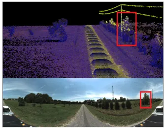
1.3 Sample point cloud data with corresponding panoramic image that cover same area. . . 5

2.1 chlorophyll is a strong absorbent of light in the red spectral band (and scat-ters only a small portion of light in this band) and heavily scatscat-ters the other parts of the spectrum, especially the NIR band. This property can be used for vegetation detection. . . 8

2.2 Top: Seven filters in visible and NIR range for the FluxData camera [1]. Bot-tom:A sample 7-band image composed of two RGB and RGB-shifted images

and one NIR image from our terrestrial multi-spectral dataset. . . 9

2.3 Top: 16 filters in the visible range for Ximea multi-spectral camera [2]. Bot-tom:A sample 16-band image from our Sydney multi-spectral dataset. Filters

are designed for active range in the visible spectrum. . . 10

2.4 Ladybug 3 camera with six 2MP cameras [3]. . . 11

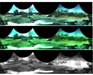
2.5 Top:360◦view Ladybug Panoramic image.Bottom:Panoramic multi-spectral

image captured by a panoramic mirror (GoPano+[4]) . . . 12

2.6 RGB-D sample images [5]. . . 13

2.7 Time-of-flight:t=2.t1=2.t2, measuring distance using a known speed light

signal between the sensor and the object. Distance is measured byD=C.t/2. 14 2.8 Velodyne 64E with rotating beam and 64 laser rays . . . 14

2.9 Sample point cloud data from our NICTA/2D3D dataset . . . 14

(16)

the neighboring pixels are connected in the graph via black lines that represent pairwise connections. The dashed lines show the scope of the cliques. Cliques are the set of nodes that are co-dependent. Bottom: The superpixel-based graphical model. In this model each superpixel is represented by a node in the graph (blue circles). Similar to the pixel-based model, each superpixel is connected to its neighbors via black lines, and cliques are the set of correlated superpixels shown via dashed lines. . . 18

2.12 Left: A sample aerial image; Right: Final land-cover classification. Classified images show Road in gray, Roof in orange and cyan, Grass in light green, Trees in dark green, Water in blue and Bare Soil in yellow. [67] . . . 20

2.13 Left Up: RGB image; Right Up: NIR image; Left Down: NDVI; and Right Down: Discrimination image for vegetation [97]. . . 21

2.14 A sample results of terrain classification [73] using a higher-order model to perform contextual classification of a 3D point cloud in an outdoor environ-ment, orange = ground, green = vegetation, dark-blue = tree-trunks/poles, sky-blue = wire, red = facade. . . 23

2.15 A sample results of 3D point cloud classification [74] using higher-order Asso-ciative Markov Networks, vegetation (green), large (red) and small (blue) tree trunks, and ground (orange). . . 23

(17)

LIST OF FIGURES xvii

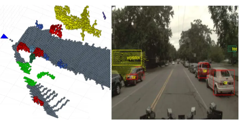
2.17 Semantic representation of one of the labeled scenes. Left image: 3D view of the inferred class labels. The blue triangle indicates the vehicle’s position. Right image: The inferred labels as well as the ROIs and the projected laser returns. The color of each ROI matches the color of the associated object in the 3D plot [29]. . . 25

2.18 The co-inference approach results in 2D and 3D data [72] using a hierar-chical labeling approach that alternatively performs classification in each do-main. Color code: purple=big-vehicle, dark-red=sidewalk, white=road, light-green=shrub, darkgreen=tree-top, brown=tree-trunk, light-red=building, pink=small-vehicle. . . 26

3.1 a) Seven Filters devised to achieve multi-spectral intensities. b) A sample 7-band image composed of two RGB and RGB-shifted images and one NIR image. c) Intensities of seven bands for a pixel within the specified white box inside the images in (b). . . 28

3.2 A general overview of our method: feature extraction, normalization and then classification using both SVM and AdaBoost. . . 28

3.3 Utilizing Fourier spectrum to estimate the fineness of the image. a) A homo-geneous image (grass). b) Fourier transform of grass. c) A detailed image of leaves. d) Fourier transform of leaves. e) The mask which is used to extract fineness feature from the Fourier spectrum. . . 29

3.4 Utilizing Fourier spectrum to find directional patterns in the image. a) Image of wood surface with a vertical pattern. b) Fourier transform of wood surface. c,d) The masks which are used to extract directional features from the Fourier spectrum. . . 31

3.5 Sample labeled multi-spectral image . . . 33

3.6 A sample of a fully labeled multi-spectral image . . . 35

4.1 A tree in the 3D point cloud data that corresponds with three different views in the panoramic images. . . 40

(18)

plane in (b). . . 45

4.6 Panoramic Ladybug images capture the 2D information of an object from dif-ferent views along the road. This enables a better understanding of the object properties. . . 46

4.7 A number of a group of successive images containing a power pole (magnified) is shown. The distribution of the feature vectors that are extracted from a spe-cific region of the power pole and from different image views is shown in a hy-pothetical multi-dimensional feature space. Despite the multi-dimensionality of the feature vectors, the feature space is shown here in two dimensions to sim-plify the illustration. In this example, the first two views are separated from the other views due to the apparent color saturation on the highlighted power poles in these views. The algorithm can easily eliminate these outliers using Equa-tion 4.2 and select a satisfying view of the power pole from {x3,x4,x5,x6}.

. . . 47

4.8 The graph of neighborhood which is used in our CRF framework. Each node (3D point) iinteracts with its adjacent nodes that are within a radius of R (illustrated with black color). . . 48

4.9 Illustration of the selected classes. The color codes are described in Table 4.1. . 49

4.10 Influence region diagram of the PFH computation for a query pointpq (illus-trated with red colour) [83]. . . 50

(19)

LIST OF FIGURES xix

5.1 The graphical model in our approach. 2D superpixels are represented by squares and 3D segments are represented by spheres. The blue edges con-nect 3D segments, green edges link 2D superpixels and double lines (in red) associate the corresponding 2D and 3D nodes. 2D and 3D nodes can be con-nected to each other, depending on their neighborhood condition and also the 2D-3D projection. . . 61

5.2 An example that illustrates how the corresponding superpixels of each 3D seg-ment and their 2D-3D pairwise weights are determined. 3D segseg-ment is pro-jected onto its nearby image planes and the superpixels that have a significant overlap with its projection are considered and the weight of pairwise links are determined according to the degree of overlap and size of the superpixels. . . . 64

5.3 An example that justifies the need for a second step normalization on 2D-3D pairwise weight vector. Since the object is very thin and the ratio of P∩A A

weakens the strength of the pairwise link between the 3D segment and its only counterpart superpixel in the image, the ratio should be normalized w.r.t. the size of the overlap. . . 64

5.4 Manual annotation of the 3D point clouds and 2D images. 1st column: Some screenshots from the 2D labeller program. 2nd column: Some screenshots from the 3D annotator program. . . 65

5.5 The qualitative results of our proposed model for semantic segmentation of (a) 2D image and (b) 3D point cloud, captured from a scene in CMU/VMR dataset. The color codes for this figure are: White=Road, Brown=TreeTrunk, Light-Red=Building, Green=TreeTop, Light-Green=Shrub, Pink=Vehicle, Red=Sidewalk, Orange=Ground, Yellow=Utility pole . . . 71

(20)

different modalities and penalize these regions for taking different labels, thus producing wrong labeling in the presence of data misalignment, or other causes of label disagreement.Bottom:Here, we introduce latent nodes that are placed

between each connected pair of 2D and 3D nodes in the graph. They explic-itly let us account for such inconsistencies, and potentially cut edges between the different domains. Circles denote the nodes in one domain (e.g., 3D) and squares denote the nodes in another domain (e.g., 2D). The latent nodes are depicted by triangles. . . 75

6.3 Top: Our model which considers 2D semantic, 3D semantic, 2D geometric

and 3D geometric nodes that are connected to each other via latent nodes. This model enables us to do inference on all the nodes using the semantic and geometric information simultaneously. Different colors represent different modalities. The latent nodes are represented by triangles. . . 76

6.4 Latent nodes for data misalignment. Left: The projection ofpolefrom 3D

to 2D covers some regions ofsky, which creates a connection between the cor-responding 3D and 2D nodes. Having access to both 3D and 2D features, the latent node should detect the mis-match and cut this connection thus allowing the nodes to take different labels. Right: In this case, the projection is

accu-rate. Therefore, the 2D and 3D features are both coherent with the class label

(21)

LIST OF FIGURES xxi

6.5 Latent nodes for moving objects. Left: Avehicle can be observed in 2D,

but was not present when the 3D laser sensor covered this area. Therefore, the label of the 3D point isroadinstead ofvehiclefor 2D. By relying on both 2D and 3D features, the latent node should predict that this connection must be cut.Middle: This represents the opposite scenario where the image depicts an

emptyroad, while the 3D points were acquired when avehiclewas passing. Here again, the latent node should cut the edge, thus allowing the nodes to take different labels. Right:In contrast, here, the 2D and 3D regions belong to the

same class and thus have coherent features. The latent node should therefore leverage this information to help predicting the correct classvehicle. . . 85

6.6 Semantic labeling vs. geometric labeling. Left: Semantic labeling Right:

Geometric labeling. This sample image shows geometric labeling in compare with semantic labeling could distinct between wire and tree leaves. . . 86

6.7 Examples of how our latent nodes improve the labeling in practice. As

shown in the 3D-2D projection, the data misalignment and object motions have caused 3D points labeled asleavesto cover thepole(top) and 3D points labeled as road to project onto the vehicles (bottom). As a consequence, with the method in our previous chapter which encourages the modalities to have the same label, the pole was labeled asleavesin 2D and the vehicle asroadin 3D (indicated by a white arrow). By contrast, thanks to our latent nodes that can cut inconsistent edges, our method produces the correct labels. . . 91

6.8 Sample results on the NICTA/2D3D dataset. 1st row: Left: 2D

ground-truth;Middle: 2D results with handcrafted potentials;Right: 2D results with

learned potentials. 2nd row: Left:3D ground-truth;Middle: 3D results with

handcrafted potentials;Right:3D results with learned potentials. This method

has been able to fix some of the mis-labelings present in our previous results with handcrafted potentials, such as the tree trunks andpolesin 2D images, andwiresandvehiclesin 3D data. Note that these are the object classes that are most likely to be affected by misalignments. . . 95

6.9 Sample results of semantic and geometric labeling in the NICTA/2D3D dataset.

1st row: image,2nd row:2D semantic ground-truth,3rd row: 2D geometric

(22)

6.11 Sample results of semantic and geometric labeling in the CMU/VMR dataset.

1st row: image,2nd row:2D semantic ground-truth,3rd row: 2D geometric

ground-truth,4th row: 2D semantic results, 5th row: 2D geometric results, 6th row: 3D semantic ground-truth,7th row: 3D semantic results,8th row:

(23)

List of Tables

3.1 The targets which were classified using the system . . . 33 3.2 The confusion matrix computed using an SVM with an RBF kernel applied to

the test data (Results are in percent and rounded) . . . 34 3.3 Confusion matrix computed using AdaBoost with 80 weak learners, applied to

the test data. (The values are in percent and rounded) . . . 37 3.4 Correlation coefficients for pixel intensities of seven bands (RGB, shifted RGB

and NIR bands) in training data. (The values are in percent and rounded) . . . . 37

4.1 The list of the classes in our classification system. . . 51 4.2 The confusion matrix computed using a CRF applied to the test data. (Results

are in percent and rounded). . . 52 4.3 The accuracy and F1-Scores of the 3D classification using single-view,

multi-view and CRF. . . 54

5.1 The F1-scores of the 2D classification for the CMU/VMR dataset ([72]) using our model with handcrafted potentials, compared to the method of [72]. The results of the 2D-only model with handcrafted potentials are provided as well for comparison. . . 68 5.2 The F1-scores of the 3D classification for the CMU/VMR dataset ([72]) using

our model with handcrafted potentials, compared to the method in [72]. The results of the 3D-only model with handcrafted potentials are provided as well for comparison. . . 68 5.3 The F1-scores of the 2D classification for NICTA/2D3D dataset using our

model with handcrafted potentials. The results of the 2D-only model with handcrafted potentials are provided as well for comparison. . . 69 5.4 The F1-scores of the 3D classification for NICTA/2D3D dataset using our

model with handcrafted potentials. The results of the 3D-only model with handcrafted potentials are provided as well for comparison. . . 70

6.1 Training and inference time for NICTA/2D3D and CMU/VMR datasets. . . . 88

(24)

the results for unary, pairwise model learned on the 2D domain only, with handcrafted potentials, the 2D-3D learned potentials, the 2D-3D learned po-tentials with latent nodes, semantic results with semantic - geometric model with and without latent nodes. . . 90 6.5 Per class F1-scores for geometric results with semantic - geometric model and

latent nodes in the NICTA/2D3D dataset. . . 91 6.6 Per class F1-scores for the 2D domain in the CMU/VMR dataset. We present

the results for unary and pairwise models learned on the 2D domain only, the method of [72], with handcrafted potentials, the 2D-3D learned potentials, the 2D3D learned potentials with latent nodes, semantic results with a semantic -geometric model with and without latent nodes. . . 92 6.7 Per class F1-scores for the 3D domain in the CMU/VMR dataset. We present

the results for unary and pairwise models learned on the 2D domain only, the method of [72], with handcrafted potentials, the 2D-3D learned potentials, the 2D3D learned potentials with latent nodes, semantic results with a semantic -geometric model with and without latent nodes. . . 93 6.8 Per class F1-scores for geometric results with semantic-geometric model and

(25)

Chapter1

Introduction

1 .

1 Motivation

Scene parsing (also known as semantic labeling) consists of assigning a class label to each element of a scene. Labeling our environment (Figure 1.1) is useful when we need to un-derstand the surrounding world in autonomous systems such as robot applications, that, e.g., can help negotiating the environment and assist blind people. Moreover, it is very helpful for other applications like intelligent vehicles (autonomous driving), automatic map generation, defect detection by capturing data periodically, and vegetation management by monitoring their growth. One of the most important components of a scene parsing system is the input data that provides information about our environment and can be obtained using various sen-sors. The most common sensor in this area of research is RGB cameras that provide color and texture information of the scene. This information is useful in classifying different objects, for example a green region with a specific texture may be classified as vegetation. Other data sensors, such as Lidar to generate 3D point cloud data, multi-spectral and thermal imaging present more information such as shape and temperature about scenes and objects.

The scene parsing task can in general be very challenging due to a number of issues in-cluding shadows and data saturation that are often seen in 2D outdoor images, occlusion and variable weather conditions. Even in ideal conditions, scene parsing is still a very compli-cated task since we face very complicompli-cated scenes. While each of the above-mentioned sensors (modalities) can alleviate some limitations of scene parsing to some extent, using multiple modalities concurrently can be more helpful. For example, if Lidar data and panoramic im-ages (360◦ images) are used together, they can cover weaknesses of each other, and as a result improve scene parsing.

Scene analysis using multiple modalities aims at leveraging complementary information captured by multiple sensing modalities, such as 3D Lidar and 2D imagery (RGB, multi-spectral and thermal). 3D data provide information about structure, shape, size and the real

(26)

Figure 1.1: Automatic outdoor scene labeling has many applications, such as in robotics, au-tonomous driving and automatic map generation [87].

(27)

§1.2 Contributions 3

In a nutshell, the goal of this thesis is to investigate the use of multiple sensing modalities to combine their information. Also we want to address some of the challenges we identified in this regard such as dealing with the misalignments between different modalities.

1 .

2 Contributions

The contributions of this thesis are on improving scene parsing by developing methods appli-cable to using multiple sensing modalities. In particular, we make the following contributions:

1.2.1 Multi-spectral Imaging for Material Classification in Scene Analysis

We investigate the potential of multi-spectral imaging for outdoor scene analysis. We propose a method suitable to distinguish between different materials occurring in natural scenes using a multi-spectral camera. Such a capability is useful in autonomous robot applications as well as in applications intended to create large scale inventories of assets in the proximity of roads. The utilized sensor records a seven band multi-spectral image, of which six bands are in the visible range and one in the near infrared (NIR) range. Figure 1.2 shows a sample image of multi-spectral data from our dataset. Many materials appearing similar if viewed by a common RGB camera, will show discriminating properties if viewed by a camera capturing a greater number of separated wavelengths. Our approach consists of combining the discriminating strength of the multi-spectral signature in each pixel and the corresponding nature of the surrounding texture. Texture features are exploited to make the system more robust to different lighting conditions.

1.2.2 Multi-view Terrain Classification using Panoramic Imagery and

Li-dar

(28)

[image:28.595.112.440.107.372.2]

Figure 1.2: Sample multi-spectral data covered 7 wavelength bands (RGB, shifted RGB and NIR).

with in a more robust fashion. This is where the contribution of our work is; that is, the de-velopment of a consensus method that can intelligently incorporate feature responses from multiple 2D views and reject those that are not very descriptive. The 3D point cloud data are then labeled using their local information as well as the information of their corresponding 2D view. Subsequently, a conditional random field (CRF) which is equipped with the probabilities of the adjacent points and confusion matrix from local classifier, is applied to the system. The experiments are performed on a challenging dataset captured both in summer and winter.

1.2.3 A Multi-modal Graphical Model for Scene Analysis

(29)

[image:29.595.148.484.110.370.2]

§1.2 Contributions 5

Figure 1.3: Sample point cloud data with corresponding panoramic image that cover same area.

leverage the information from its corresponding regions in the other modality to better esti-mate its class label. We evaluate our method on a publicly available dataset. Additionally, to demonstrate the ability of our model to support multiple correspondences for objects in 3D and 2D domains, we introduce a new multi-modal dataset. This dataset consists of panoramic images and 3D point cloud data captured from outdoor scenes (NICTA/2D3D Dataset). The data includes the entire set of 3D points which provides naturally occurring many-to-one re-lationships. That is, each 3D point is seen from a number of 2D images. The images have both a large vertical and horizontal Field of View (FOV) of the associated point cloud data, providing an opportunity to establish correspondences between 3D points and imagery from a large number of view points. We have made this dataset publicly available1_{. This enables} research on methods necessary to resolve issues with ambiguity, occlusions that are spurious or due to parallax, and missing 2D-3D correspondences.

1.2.4 Soft Correspondences in Multi-modal Scene Parsing

We improved our multi-modal graphical model to better address the problems of data mis-alignment and label inconsistencies in semantic labeling by introducing latent nodes to

(30)

taneous 2D/3D semantic and 2D/3D geometric inference, we perform simultaneous inference of semantic and geometric classes both in 2D and 3D that leads to satisfactory improvements of the labeling results in both datasets. Note that geometric classes are specified based on the geometric shapes of the scene elements, which include vertical planes, horizontal planes or cylindrical objects.

1 .

3 Thesis Outline

(31)

Chapter2

Background and Related Work

In this chapter, we briefly introduce 2D and 3D modalities for scene understanding. Then, we review the literature and present the previous works on outdoor scene understanding using multiple modalities.

2 .

1 Sensory Modalities

There are different sensing modalities to capture information from our environments, e.g., vi-sual and auditory modalities. In this work, we concentrate on 2D modalities, such as RGB and multi-spectral imaging, and 3D modalities such as depth and Lidar sensors for scene under-standing.

2.1.1 2D Modalities

2D imaging has been widely used for decades and its use for scene analysis has been demon-strated convincingly [64, 54, 63]. For example, common cameras that provide color measure-ments (RGB) can be used for object classification by extracting texture information for the observed object. Multi-spectral imaging and panoramic imagery constitute other examples. The former captures additional wavelength bands compared to RGB imaging, and the latter provides wide horizontal view images. We further discuss these 2D imaging modalities in the following sub-sections.

2.1.1.1 Multi-spectral Imaging and RGB

Multi-spectral imaging typically facilitates capturing 2D information of objects in several par-ticular wavelength bands including bands in the visible and invisible light ranges. RGB imag-ing can then be considered a simple type of multi-spectral imagimag-ing with three wide bands corresponding to the wavelengths of Red,Green and Blue light. Compared to RGB imaging,

(32)

Figure 2.1: chlorophyll is a strong absorbent of light in the red spectral band (and scatters only a small portion of light in this band) and heavily scatters the other parts of the spectrum,

especially the NIR band. This property can be used for vegetation detection.

multi-spectral imaging extracts additional information that the human eyes are often incapable of capturing. Various objects may show different spectral responses in different wavelength bands depending on their materials. This property that gives a unique spectral signature to each material, has been used for object classification [103, 102, 20]. One of the applications of multi-spectral imaging is in vegetation detection. Vegetation is chlorophyll-rich [23] and chlorophyll is a strong absorbent of light in the red spectral band and heavily scatters the other parts of the spectrum, especially the Near Infrared (NIR) band (Figure 2.1).

Figure 2.2 shows the seven filters used for the FluxData camera and a sample seven-band multi-spectral image composed of RGB, RGB-shifted (An image with three channels similar to RGB, with the difference that the wavelength bands are shifted in the spectrum, compared to the standard RGB wavelength bands) and NIR images. As another example, Figure 2.3 presents sample images from a sixteen-band Xiema camera [2] and the corresponding filters.

2.1.1.2 Panoramic Imagery

(33)

[image:33.595.205.430.232.563.2]

§2.1 Sensory Modalities 9

Figure 2.2:Top: Seven filters in visible and NIR range for the FluxData camera [1].Bottom:

(34)

[image:34.595.77.511.187.598.2]

Figure 2.3:Top:16 filters in the visible range for Ximea multi-spectral camera [2].Bottom:A

(35)

[image:35.595.263.371.117.224.2]

§2.1 Sensory Modalities 11

Figure 2.4: Ladybug 3 camera with six 2MP cameras [3].

cameras enable the system to collect video from more than 80 % of the full360◦sphere. To obtain panoramic multi-spectral images for the purpose of the work in this thesis, in-stead of using several multi-spectral cameras that can be very costly, a multi-spectral camera is fitted with a panoramic mirror (GoPano+) to enable a360◦view. Panoramic imaging, in addi-tion to providing a full view of our environment, is suitable to fuse with 3D Lidar point cloud data, as they both typically provide360◦ coverage. Figure 2.5 shows two sample panoramic images. The top image was captured by the Ladybug camera and the bottom one is a multi-spectral image that was captured using a panoramic mirror. The panoramic images captured by ladybug camera typically have distortions in areas where sub-images are stitched together. The black regions in the panoramic images produced by the panoramic mirrors are the results of dewarping process.

2.1.2 3D Modalities

3D sensors provide 3-dimensional information about our environment by measuring distance between objects and the sensor. Having access to 3D data can be very beneficial for scene analysis due to its potential in providing shape, size and distance information. Two widely used 3D modalities are RGB-D cameras and Lidar sensors, which we describe below.

2.1.2.1 RGB-D Imaging

(36)

[image:36.595.133.419.118.321.2]

Figure 2.5: Top: 360◦ view Ladybug Panoramic image. Bottom: Panoramic multi-spectral

image captured by a panoramic mirror (GoPano+[4]) (In this image just three bands in the RGB range are presented).

map is constructed by analyzing a speckle pattern of infrared laser light. The technique of analyzing a known pattern is called structured light [70]. The general principle of structured light is to project a known pattern onto the scene and infer depth from the deformation of that pattern. The Kinect takes advantage of structured light using two computer vision techniques, depth from focus, and depth from stereo [70]. Depth from focus exploits the fact that blur increases with distance and depth from stereo relies on the fact that the horizontal shift of a point observed from two different view points is inversely proportional to its distance to the camera. Figure 2.6 shows a sample RGB-D image. RGB-D cameras have been extensively used for indoor scene analysis due to their ease of access and use. However, their limitations in maximum distance coverage (around 4-5 meters), small field of view (57.8◦) [6] and also low resolution make them inapplicable for our purpose of outdoor scene understanding. Note that, since RGB-D images are 2D images that contain distance information, they are usually called 2.5D data, where the 3D environment of the observer is projected onto the 2D planes of the retina.

2.1.2.2 Lidar Sensor

(37)

§2.2 Multiple Sensory Modalities 13

Figure 2.6: RGB-D sample images [5].

distance to objects are computed, given the time-of-flight of the signal travelled between the sensor and the object (Figure 2.7). Lidar uses near infrared light for this measurement (Ultra-violet and visible lights are also used for specific applications). It can target a wide range of materials, including non-metallic objects, rocks and trees. For terrestrial outdoor mapping, the Velodyne [7] sensor is a common choice. The Velodyne sensor scans the area using a rotating beam with individual 32 or 64 laser rays and has been widely applied in the applications such as the autonomously driving Google car [8]. In the Velodyne 64E [9], 64 lasers are mounted on the sensor and the entire unit spins. This allows for 64 separate lasers, each firing thousands of times per second, thus providing a rich point cloud. The unit inherently delivers a360◦ hor-izontal field of view (FOV) and26.8◦vertical FOV [9]. This sensor is able to provide returns from surfaces up to 120 meters away. Note that since the point cloud is built by a rotating sensor, it may miss fast moving objects. Figure 2.8 shows the Velodyne 64E sensor that has been used for our dataset and Figure 2.9 presents sample point cloud data from our dataset. Note that a new technology (called Solid-State-Lidar) is coming, making 3D Lidar viable in consumer products. It has no moving part and uses an optical phased array as a transmitter which can steer pulses of light by shifting the phase of a laser pulse as it is projected through the array1_.

2 .

2 Multiple Sensory Modalities

Different modalities with their specific properties can help to capture certain properties of the environment. For example, 2D imaging provides information such as color and texture, 3D data supplies distance information, which in turn can be used to infer shape and size cues. Capturing data simultaneously with several modalities provides a rich source of information

(38)

[image:38.595.245.326.315.428.2]

Figure 2.7: Time-of-flight: t = 2.t1 = 2.t2, measuring distance using a known speed light

signal between the sensor and the object. Distance is measured byD=C.t/2.

Figure 2.8: Velodyne 64E with rotating beam and 64 laser rays

[image:38.595.75.486.467.696.2]

(39)

§2.2 Multiple Sensory Modalities 15

about our environment that can improve classification results [30, 72]. The systems produc-ing these data modalities are often mounted on a platform on a surveyproduc-ing vehicle to record the multi-modal data. Although employing several modalities is helpful for scene analysis, their different properties, data capturing methods and locations create new challenges. The multi-modal data should be aligned/registered with each other to enable their joint analysis. Alignment/registration is the process of putting all the various modalities data into the same coordinate system. It is important to note that even with a good registration/alignment between modalities, their corresponding elements may point to different items in the scene due to the different properties of the modalities. For example fast moving objects are often not captured correctly in Lidar data due to its rotating capture system.

2.2.1 Registration

(40)

Figure 2.10: Three examples of misalignment between 2D and 3D data. Left: The projection of pole from 3D to 2D covers some regions of sky. Middle: A vehicle can be observed in 2D, but was not present when the 3D laser sensor covered this area. Right: This represents the opposite scenario where the image depicts an empty road, while the 3D points were acquired

when a vehicle was passing.

2 .

3 Approaches to Scene Understanding

2.3.1 2D Scene Understanding

Scene understanding from 2D imagery has been intensely studied, yielding increasingly accu-rate results [92, 112, 57, 35, 114, 49]. Scene analysis using 2D images alone is ,however, not the subject of this thesis and while there is a large body of work on this topic, in this section, I focus the discussion on the most related works, especially the ones that utilize Conditional Random Field (CRF) to leverage the contextual information of the scene. The related work on multi-spectral imaging is reviewed in Section 2.3.1.1.

(41)

dif-§2.3 Approaches to Scene Understanding 17

ferent environmental conditions. They extracted color and wavelet features from the luma and chroma color space (YUV) and also spatial coordinates of the objects. They then classified the data using Neural Networks [93], SVM and a Maximum Likelihood classifier with Gaussian Mixture Models (GMM-ML) [47].

The classifiers that just consider the local information of the scene are calledunary classi-fiers in which the labeling of each element is done independently of the other elements in the scene. These classifiers in most cases are not strong enough to classify the elements well and are heavily vulnerable to noise. In order to improve the results attained by the unary classifiers, higher-level knowledge, such as contextual information, can be leveraged by using graphical models and CRF in particular.

A CRF [58] (Figure 2.11) models a labeling problem with a graph where each node is one of the data elements, Pixels or superpixels. In this graph, the label of each node is dependent of its local evidence (result of the unary classifier) and the status of its neighbors. A set of nodes that have similar features is called aclique. A CRF formulation may consist of unary poten-tials, pairwise potentials and higher-order potentials. The unary potential indicates the cost of assigning a label to a single node and can be computed using the result of the unary classifier. Pairwise potentials and higher-order potentials however determine the cost of assigning a label combination to two nodes and a clique of more than two nodes, respectively. The nodes of a clique are conditionally dependent of each other. Let x = {xi} , 1 ≤ i ≤ N, be the set

of features extracted from N elements of the data andy = {yi} , 1 ≤ i ≤ N, be the set

of variables encoding the labels of the nodes, where each variable can take a label in the set

L={1,· · · ,L}. Then, the joint distribution of all modalities conditioned on the features can be expressed as

P(y|x) = 1

Z ·exp

−(

N

∑

i=1

Φi+

∑

(i,j)∈E

Ψij+

∑

c∈C

Ψc)

, (2.1)

where Z is the partition function and Φ denotes the unary potentials. Ψij denotes pairwise

potentials defined over the set of edgesE andΨcdenotes higher-order potentials defined over

(42)

[image:42.595.78.488.125.568.2]

Figure 2.11: Middle: A sample of a segmented scene where the superpixels are presented by red lines. This image is zoomed in, so it appears blurry. Top: The pixel-based graphical model. Each pixel is denoted by a node in the graph (blue circles), all the neighboring pixels are connected in the graph via black lines that represent pairwise connections. The dashed lines show the scope of the cliques. Cliques are the set of nodes that are co-dependent. Bottom: The superpixel-based graphical model. In this model each superpixel is represented by a node in the graph (blue circles). Similar to the pixel-based model, each superpixel is connected to its neighbors via black lines, and cliques are the set of correlated superpixels shown via dashed

(43)

§2.3 Approaches to Scene Understanding 19

modeled using pairwise potentials. [53] proposed a method for learning the label compatibility knowledge that can be applied to a fully connected CRF. In addition, higher-order models [48, 49, 51, 55, 105, 107] were used to capture higher-order relationships between the elements in the scene. [48] introduced the Pn Potts model to model higher-order relationships that

encourage all the pixels within one image patch to take the same class label. [51] presented Pattern-based potentials for higher-order models, where higher-order cliques are encouraged to follow one of the library patterns that are learned previously.

2.3.1.1 Multi-spectral Imaging

Despite the useful information provided by RGB cameras, the information from a wide range of the light spectrum is not recorded using this data modality. With the prospect of low-cost multi-spectral imaging around the corner, a vast array of potential applications has opened up. By considering reflections of a material in different spectral sub-bands, material identification will be more tractable. As a result, multi-spectral imaging can facilitate object recognition tasks based on which material they are made. For example, objects that look the same to the naked eye may in fact look very different if the reflected light is sampled in more bands than the typical three bands that an RGB camera provides.

(44)

Water in blue and Bare Soil in yellow. [67]

In [84], material classification using multi-spectral images was performed indoors, for a few classes, and without the challenges of outdoor lighting. The authors in [18] and [85] ex-ploited multi-spectral imaging for scene recognition and image categorization, respectively. While scene recognition and image categorization are important tasks, the problem of material classification is not being addressed. Outdoor terrain classification aided by multi-spectral im-ages is addressed by [97, 16], however, only vegetation detection is considered. Additionally, aerial spectral imaging has been utilized in some terrain and urban environment classification tasks. Lizarazo et al. [67] classified urban land-cover into roads, rooftops, grass, trees, water body and soil, using RGB and NIR aerial images, by applying a fuzzy segmentation method. A sample of their aerial dataset and the classification results are shown in Figure 2.12. Fauvel et al. [32] classified urban area to different categories such as asphalt, metal sheet, brick and other terrain parts. They employed 115-band hyper-spectral aerial data, exploited spatial infor-mation and learned an SVM based classifier.

(45)

Figure 2.13: Left Up: RGB image; Right Up: NIR image; Left Down: NDVI; and Right Down: Discrimination image for vegetation [97].

2.3.2 3D Scene Understanding

2D features are often insufficient to describe objects and 3D shape information can help dis-ambiguate between objects that would appear very similar in 2D. For example, a concrete wall can easily be distinguished from a concrete road using 3D shape features. Unfortunately, ac-quiring accurate and dense 3D shape features from a sequence of sparsely collected images is difficult or even impossible. In order to capture the 3D information of the scenes, Lidar systems have been widely used to create so called point clouds. Lalonde [60] used a Bayesian classifier operating on saliency features measuring the local point cloud distribution to classify natural terrain. They identified three general classes of objects which had scattered (like grass and bushes), linear (like tree branches) and planar (ground surface and big rocks) point cloud distributions. They measured the spatial distribution of the points in a local neighborhood by computing the eigenvalues of a 3D covariance matrix of each region. Saliency features were then constructed from these eigenvalues by fitting a Gaussian Mixture Model (GMM) [14] to the training dataset using Expectation Maximization [26]. Jutzi and Gross [45] classified the point clouds of urban buildings into general structural classes, such as edge, corner and plane, by assigning 3D spherical neighborhood volumes to each point and computing the eigenvalues of point distributions within this volume. They also estimated 3D contours of the objects by considering consecutive points with a similar eigenvector. These works attempted to classify the point cloud data into some generic point distribution categories and did not assign semantic class labels to the points.

(46)

can-give, they are relatively sparse and carry noise from, for example, scan misalignment and error in distance estimates. This leads to difficulties such as accurately segmenting and classifying complex outdoor scenes where the magnitude of the noise is sometimes similar to the size of the objects of interest. Furthermore, if two objects are located too close to each other, the 3D points may not be able to distinguish them appropriately. [11, 65, 69, 77] have worked on pairwise graphical models on point cloud data and improved the classification accuracy signif-icantly. Munoz et al. [73] used a higher-order model to perform contextual classification of a 3D point cloud in an outdoor environment. The Markov Random Field [65] is used as their model to consider contextual information and the parameters of this model was defined by a functional gradient approach. Also these authors [74] used higher-order Associative Markov Networks on 3D outdoor point clouds. They defined their high-order cliques in the 3D point cloud as a set of locally similar points obtained by k-means clustering [46] over the points’ fea-tures and locations. For their clique potentials, they considered similar potentials to the work in [48] calledPnPotts model. This associative model favors all variables in the clique taking

on the same label. Xiong et al. [113] used a sequence of hierarchical classifiers at different scales (region-wise and point-wise) where the class predictions of each classifier was given as a feature-set to the classifier in the next stage. Then, through an iterative process of going back and forth between the stages, they predicted the final labeling of the 3D point cloud data with some promising results. However, the convergence of their method should be investigated when dealing with a large number of class labels. In Figure 2.14, Figure 2.15 and Figure 2.16 we show some results of [73], [74] and [113], respectively.

2.3.3 Multiple Modalities

(47)

comple-§2.3 Approaches to Scene Understanding 23

Figure 2.14: A sample results of terrain classification [73] using a higher-order model to per-form contextual classification of a 3D point cloud in an outdoor environment, orange = ground,

green = vegetation, dark-blue = tree-trunks/poles, sky-blue = wire, red = facade.

Figure 2.15: A sample results of 3D point cloud classification [74] using higher-order Associa-tive Markov Networks, vegetation (green), large (red) and small (blue) tree trunks, and ground

(48)

[image:48.595.151.398.111.342.2]

Figure 2.16: Example results of 3D point cloud classification [113] from VMR-Oakland-v2 dataset using a sequence of hierarchical classifiers at different scales (region-wise and point-wise), grey = ground, light-red = building, brown = tree-trunk, dark-green = vegetation, pink

= vehicle, dark-blue = pole, lightblue = wire [113].

(49)

[image:49.595.116.527.105.314.2]

Figure 2.17: Semantic representation of one of the labeled scenes. Left image: 3D view of the inferred class labels. The blue triangle indicates the vehicle’s position. Right image: The inferred labels as well as the ROIs and the projected laser returns. The color of each ROI

matches the color of the associated object in the 3D plot [29].

will thus mis-classify some regions in at least one of the domains.

(50)

purple=big-vehicle, dark-red=sidewalk, white=road, light-green=shrub, darkgreen=tree-top, brown=tree-trunk, light-red=building, pink=small-vehicle.

speed. To give a concrete example, in the NICTA/2D3D dataset, 17% of the connections between the two modalities correspond to inconsistent labels. As a consequence, since existing methods fail to model these inconsistencies, they will typically produce wrong labels in at least one modality.

(51)

Chapter3

Multi-spectral Imaging for Materials

Classification in Scene Analysis

In this chapter, we investigate the potential of multi-spectral imaging for outdoor scene un-derstanding. A method suitable for distinguishing between different materials appearing in natural scenes using such a multi-spectral camera is devised. The application we have in mind is a system capturing natural outdoor imagery in road scenes, and we are interested in classi-fying the objects in the environment based on their material. This kind of information is useful to, e.g., create large scale inventories of materials for road asset management and vegetation management.

Considering the RGB based approaches [22, 47] and their inherent limitations in material identification, we propose an automatic system for material classification in natural environ-ments by using multi-spectral images alone. Multi-spectral cameras are still expensive but will be commonplace and cheap in the next few years thanks to the technology evolution. The rest of this chapter is organized as follows. Section 3.1 describes the capture platform and the as-sociated data which have been used. Next, we introduce our approach in Section 3.2 and our experimental results in Section 3.3. The last section provides a summary.

3 .

1 Data Capture System

The multi-spectral imagery studied in this chapter was recorded from the roads around Can-berra, using a FluxDataTM _{[1] camera configured to capture seven frequency bands. Six of}

the bands are in the visual range and one band is in the NIR range. Figure 3.1-a gives an overview of the bands and respective photon efficiency. The camera uses three individual 2M pixel sensors which capture 3, 3 and 1 bands, respectively.

The FluxDataTM_{camera was fitted with a panoramic mirror (}_GoPano+_{) to enable a}₃₆₀◦

(52)

Figure 3.1: a) Seven Filters devised to achieve multi-spectral intensities. b) A sample 7-band image composed of two RGB and RGB-shifted images and one NIR image. c) Intensities of

seven bands for a pixel within the specified white box inside the images in (b).

AdaBoost

Normalization

Feature

Extraction

SVM

Figure 3.2: A general overview of our method: feature extraction, normalization and then classification using both SVM and AdaBoost.

view, and subsequently attached to the surveying vehicle. In a post processing step, the spherical images were unwarped by a software package associated with GoPano+, creating panoramic images of 1241×4176 pixels. Images were taken approximately every 2.7 meters along the road. Figure 3.1-b shows a sample image from this setup, in which, a pixel is selected and its multi-spectral signature is illustrated in Figure 3.1-c.

3 .

2 Method

The method is comprised of three stages; feature extraction, normalization and then classifica-tion. In the classification stage, both SVM and AdaBoost [33] are presented. Figure 3.2 shows an overview of our method.

3.2.1 Feature Extraction

(53)

§3.2 Method 29

Figure 3.3: Utilizing Fourier spectrum to estimate the fineness of the image. a) A homoge-neous image (grass). b) Fourier transform of grass. c) A detailed image of leaves. d) Fourier transform of leaves. e) The mask which is used to extract fineness feature from the Fourier

spectrum.

3.2.1.1 Pixel-level features

These features are extracted from the information at a single pixel location. They are:

-Intensity features:

For each pixel, we store the seven intensities obtained from the seven bands of the sensor.

-Normalized Difference Vegetation Index (NDVI):

One of the most important characteristics of vegetation is that it is chlorophyll-rich [23]. Chlorophyll is a strong absorbent of light in the red spectral band. On the other hand, it heavily scatters the other parts of the spectrum, especially the NIR band. From these observations, vegetations can be detected using [101]

NDV I = ρN IR−ρRED ρN IR+ρRED

, (3.1)

whereρN IRandρREDrepresent the spectral reflectance in the NIR and Red bands, respectively.

It can be demonstrated that, for vegetation regions, NDVI is approximately+1.

3.2.1.2 Region-level features

The following features are extracted from a block of radiusRaround the pixel of interest. -Mean and Standard Deviation:

(54)

from the number of intensity levels in the image, and not from the intensity values. As a re-sult, multiplying the whole image by a coefficient does not affect the co-occurrence matrix. It makes this matrix suitable to classify similar objects in different lighting conditions. In total, 42 features from 7 bands are computed for each pixel.

-Fourier Spectrum:

The Fourier transform [44] of the image can be used to indicate some properties of the image as well [61]. For example, the fineness of the picture can be estimated by examining how much spectrum of Fourier transform is focused around the center. A smooth image has an almost compact Fourier spectrum. However, the presence of details in the image results in a more scattered Fourier transform. Figure 3.3 shows that the more detailed image has a sparser Fourier spectrum. A measure of sparseness of the Fourier spectrum can be obtained by applying a mask to keep the information in the mid-frequency bands. This mask is presented in Figure 3.3-e.

Furthermore, the Fourier spectrum also defines directional texture very well. In Figure 3.4, we can see that vertical texture in the image of wood gives rise to a horizontal pattern in its Fourier transform. The masks that are used to extract directional features from the image blocks are shown in Figure 3.4-c,d.

In the above, the masks are embedded in neighborhood blocks of radius R. The mean

of the intensity of the pixels inside these masks are extracted as Fourier features. To make these features independent of the intensity scaling, they are divided by the mean value of their corresponding block. In total, 28 features from 7 bands are computed for each pixel.

(55)

§3.2 Method 31

Figure 3.4: Utilizing Fourier spectrum to find directional patterns in the image. a) Image of wood surface with a vertical pattern. b) Fourier transform of wood surface. c,d) The masks

which are used to extract directional features from the Fourier spectrum.

3.2.2 Classification

Although SVM and AdaBoost are well-known classification methods, in this section, we briefly describe these classifiers that were used in this chapter.

3.2.2.1 Support Vector Machine (SVM)

The SVM classifier attempts to find the hyperplane that divides the data points into their correct classes with the maximum possible margin:

min

w,b,ξ

1 2w

T_w₊_C T

∑

i=1

ξi (3.2)

s.t.: y_i(wTx_i+b)≥1−ξ_i, ξ_i ≥0, ∀i=1, 2, . . . ,N , (3.3)

whereNis the number of training data. Here we make use of kernel SVM with a Radial Basis

Function (RBF) kernel:

K(xi,xj) =exp

− kxi−xjk 2

2σ2

(3.4)

This kernel is applied to the 85-dimensional features discussed in Section 3.2.1. Parametersγ andCare optimized using validation data. We make use of theLIBSVM MATLABTMtoolbox

(56)

classification:

ht(x) =

 



1 ft(x)<θt

0 Otherwise (3.6)

Note that a feature may be used more than once as a weak learner, with different thresholds.

3 .

3 Experimental Results

The system was implemented inMATLABTM_{. The dataset includes 169 images. We select}

ten classes as the targets for classification. Table 3.1 shows the assigned classes with their corresponding colors used for labeling the images. This label assignment can be observed in Figure 3.5. Note that, in addition tograssandroad, four more classes, i.e.,leaves,tree trunks,

white lines, andlight poles and road guardssuffer from shadows. However, no separate class was assigned to them due to the difficulties of accurate manual labeling.

All 169 images underwent a labeling process based on the color codes in Table 3.1 and some regions from each class were labeled. 10 images were selected as the validation data for tuning the parameters of the models and features. In the next step, from the training data, 15,000 pixels from each class (150,000 in total) were randomly picked for the feature extraction part. 85 features, as explained above, were obtained for each pixel and for different block sizes, fromR=4toR=15. The best block size was chosen later, in the validation process for each classifier. Afterwards, we conduct 5-fold cross-validation in order to reduce the overfitting.

SVM: We apply an SVM classifier with an RBF kernel for training with different block

sizes and different model parameters. These parameters were optimized using the validation data. The best validation accuracy1 _{was achieved for the neighborhood block with a pixel} radius ofR=8and also forC=4andσ =0.04. ChoosingR=8seems reasonable because a very large block size leads to a smoothly labeled image which might be wrongly classified at

(57)

[image:57.595.114.507.131.492.2]

§3.3 Experimental Results 33

Table 3.1: The targets which were classified using the system Class number Class name and color

1 Tree trunks:dark brown

2 Light poles and road guards: blue 3 Shadow on the grass: dark blue

4 Grass: dark green

5 Road: brown

6 White lines on the road: red 7 Shadow on the road: yellow

8 Leaves: green

9 Sky:light blue

10 Clouds and white regions in the sky: Purple

Figure 3.5: Sample labeled multi-spectral image

the edges, while selecting a very small neighborhood block results in a noisy labeled image. The computed SVM model was employed to classify the test data and the accuracy was computed to be 92.9%. Table 3.2 shows the resulting confusion matrix of the SVM classifica-tion. Note that almost all classes were considerably distinguished from each other, despite the presence of shadows in most of the classes and also the similarity of pixel intensities between some of them. For example, although there is a high similarity between the pixel intensities of

grassandleaves, these two classes have been discriminated down to an error of less than 2%. Furthermore, the system has been able to classifyshadow on roadandshadow on grassregions relatively well, using the features of Section 3.2.1. This clearly demonstrates the usefulness of texture features.

(58)

Road 0 0 1 1 98 0 0 0 0 0

White lines 1 0 0 0 0 99 0 0 0 0

Shadow-road 1 1 4 0 2 0 92 0 0 0

Leaves 2 0 4 1 0 0 0 93 0 0

Sky 0 0 0 0 0 0 0 0 100 0

Clouds 0 1 0 0 0 3 0 0 0 96

91.9%. The difference between the maximum and minimum of classification accuracies for each class in cross validation was negligible.

AdaBoost: The number of weak learners selected by AdaBoost can often be significantly

fewer than what is available in the pool of features. Finding an appropriate number of weak learners of the resulting strong classifier is done by measuring the performance of the strong classifier as a function of its size using the validation data. The feature pool consisted of a total of 85 features. The optimal number of weak learners turned out to be 80. Note thatR= 8was also found to be the best block size, as in the case of SVM.

Classification of the test data using the AdaBoost strong classifier with 80 weak learners resulted in an accuracy of 89.1%. A confusion matrix for this classifier is shown in Table 3.3. Furthermore, the average accuracy of 5-fold cross-validation using the AdaBoost classifier was 89.1%.

Full image labeling:Figure 3.6 shows a fully labeled image using the SVM classifier. The

saturated pixels in the middle of the road are removed from the classification and indicated by black pixels. Clearly, our automatic approach shows great potential to discriminate between different classes in natural scenes.

Importance of sub-bands: Further experiments were made to establish the relative

[image:58.595.78.480.151.359.2]

(59)

[image:59.595.126.508.106.311.2]

§3.4 Summary 35

Figure 3.6: A sample of a fully labeled multi-spectral image

the intensities of the NIR image and the 6 visible range images are very low, compared to the correlation coefficients among the intensities in the visible spectrum images.

It shows that the image extracted from the NIR band can bring a considerable amount of information to the system and improve its accuracy. This result supports the previous studies [84, 18, 85, 96, 16] in which augmenting the NIR data led to a more accurate system.

3 .

4 Summary

In this chapter, as a first investigation into the utility of multi-spectral camera for material identification, we have proposed a method for discriminating between various materials in natural scenes based on imagery captured using a multi-spectral camera. In addition to the regular RGB spectrum, three visible sub-bands and one NIR sub-band were captured. This extra information and specifically the NIR image offer an improved classification system for distinguishing a variety of outdoor materials and objects. We extract the local texture features from 7 spectral bands for each pixel. We choose SVM and AdaBoost for classification, thanks to their great potential in to generalize. As a result, the test data were classified into ten pre-defined classes using SVM and AdaBoost with the average cross-validation accuracies of 91.9% and 89.1%, respectively. The results inImportance of sub-bandsdemonstrates the

significance of multi-spectral imaging compared to using traditional RGB cameras.

(60)

in this thesis. However, while there is no great novelty, the material lends itself to explain the general area of interest.

(61)

§3.4 Summary 37

Table 3.3: Confusion matrix computed using AdaBoost with 80 weak learners, applied to the test data. (The values are in percent and rounded)

TreetrunksPoles Shado

w-grass

Grass Road White

lines Shado

w-road

Leaves Sky Clouds

Tree trunks 82 7 5 1 0 1 0 4 0 0

poles 13 78 1 0 3 5 0 0 0 0

Shadow-grass 10 3 63 0 0 0 21 3 0 0

Grass 0 0 0 97 0 0 0 3 0 0

Road 0 0 3 2 94 1 0 0 0 0

White lines 0 4 0 0 1 95 0 0 0 0

Shadow-road 3 4 7 0 0 0 86 0 0 0

Leaves 3 0 4 2 0 0 0 91 0 0

Sky 0 0 0 0 0 0 0 0 100 0

Clouds 0 1 0 0 0 3 0 0 0 96

Table 3.4: Correlation coefficients for pixel intensities of seven bands (RGB, shifted RGB and NIR bands) in training data. (The values are in percent and rounded)

Red Green Blue Shifted-RedShifted-GreenShifted-BlueNIR

Red 100 - - -

-Green 92 100 - - - -

-Blue 87 95 100 - - -

-Shifted-Red 98 89 86 100 - -

-Shifted-Green 88 98 90 87 100 -

-Shifted-Blue 80 88 96 81 83 100

(62)

(63)

Chapter4

Multi-view Terrain Classification

using Panoramic Imagery and Lidar

After investigating the potential of multi-spectral imaging for outdoor scene understanding, in this chapter, we study 3D point cloud data for terrain classification and more specifically, how to improve 3D data classification using multi-view 2D information. In particular, we make use of terrestrial Lidar data and panoramic RGB images. Unlike indoor object classification, a system which is designed for the classification of outdoor environments should deal with many unavoidable issues such as occlusion, very complex scenes, variable weather conditions and also misalignment between the different data modalities. We devise a new framework to im-prove the classification and make it more robust against these issues that has many applications in natural scene classification tasks and robotics. In Section 4.1, we discuss the challenges of outdoor scene understanding especially using multiple modalities. The datasets and capture platform used in this work are introduced in Section 4.2 and then we describe the proposed approach. Finally, the performance of the proposed method is presented in Section 4.4.

4 .

1 Multi-view Outdoor Scene Understanding

It can indeed be useful to combine image data with Lidar. However, a common problem with the current state-of-the-art approaches is that the imagery is single-view only. If an object is partly or completely occluded in that view, the detection and classification of that object will be difficult, if not impossible.

Furthermore, a natural effect that is often seen in 2D outdoor images are dark shadows in parts of the image, which make some objects difficult to recognize. In addition, the excessive amount of light in some image areas gives rise to color saturation, which in turn, results in loss of information in those image regions.

Scene Parsing using Multiple Modalities