Seismic body wave attenuation in the upper mantle beneath the Australian continent

Seismic Body Wave Attenuation

in

the Upper Mantle beneath

the Australian Continent

by

Hai-Xu Cheng

A thesis submitted for the degree of Doctor of Philosophy

of

The Australian National University

Author's Declaration

Except as noted throughout the text and in the acknowledgments, the research described in this thesis is solely that of the author.

~

$rt(m

cf~~~

HAI-XU CHENG

The Australian National University

Contents

Acknowledgments

Abstract

I Introduction

Chapter 1 Introduction

1.1 The SKIPPY and KIMBA Projects . . . . 1.2 The Scope of the Thesis

.

IX

XI

1

2

2

4

Chapter 2 Q 8

2.1 Attenuation Terms and Definition of Q . . . 9

2.1.1 Definition of Q . . . . 2.1.2 Intrinsic Attenuation and Scattering . 2.1.3 Frequency Dependence of Intrinsic Q .. 9 . . . 10

· · · · . . . 11

2.1.4 Previous Seismological Studies on Frequency Dependence of Body Wave Attenuation . . . 16

19 2.2 Physical Mechanisms of Seismic Wave Attenuation 2.2.1 Physical Mechanisms of Attenuation . . . 19

2.2.2 Laboratory Measurement of Attenuation and Dispersion . . . 20

2.2.3 Application to Seismological Models for the Earth's Interior . . . 23

2.3 Q Models in the Upper Mantle on Global and Regional Scales . . . 24

2.3.1 Introduction . . . 24

2.3.2 1-D Q Models in the Earth . . . 2 5 2.3.3 3-D Tomographic Q Models in the Earth . . . 2 5 2.3.4 Previous Studies of Attenuation Structure in the Upper Mantle beneath the Australian Continent . . . 26

CONTENTS

Chapter 3 P and S Velocity Structure under Australian Region and their Geological Background

3.1 Geological Background of the Australian Continent

3.2 P and S Velocity Structure in the Upper Mantle .. 3.3 Discussion . . . .

II Spectral Theory and Numerical Simulation of

bt;P

Chapter 4 Numerical Simulation of Seismic Wavefield, Travel-time and t* 4.1 Introduction . . . .

4.2 Ray Presentation of Regional Propagation

4.3 Numerical Simulation of Travel-time . . .

4.3.1 Velocity and Q Models for Calculating Travel-time and t *

4.3.2 Travel-time as a Function of Distance .

4.3.3 Slowness as a Function of Distance

4.4 Numerical Simulation oft; , tJ and 8tJP

4.4.1 The t; and tJ as a Function of Distance

4.4.2 The t; and tJ as a Function of Slowness .

. . . . .

. . . . .

. . . . .

. . . . .

V

29

29

31

39

40

41

41

42

42

43

45

46

46

46

47

4.4.3 The 8tJP Calculated from Velocity and Q Models akl35, sk14 and pkq 48

4.4.4 8tJp Behaviour Interpretation. . . 49

4.5 Effects of Source Depth on Travel-time and t * . 50

4.5.1 The Effects of Source Depth on Travel-time . 50

4.5.2 The Effect of Source Depth on t; and tJ

4.5.3 Influence of Heterogeneity on Travel-time and t *

4.6 Discussion . . . .

50

52

52

Chapter 5 The Spectral Theory and the 8t* Measurement Techniques 53

5.1 Introduction. . . 53

5.2 Spectral theory and t* definition . 54

5.2.l Techniques for Measurement of Differential Attenuation 8tJp 56

5.2.2 Path Average Properties of Frequency Dependence of Attenuation. . . 59

5.3 Discussion on the assumptions involved . . . 61

5.3.1 Instrumental Response and Crustal Transfer Functions for P and S Waves 61

5.3.2 Relation between Q₅ and Qp . . . .

5.3.3 Relation between V5 and Vp and ray divergence factor .

61

CONTENTS

5.3.4 Source Spectra for P and S Waves . . . 5.4 Experiments on c5t* Measurement Procedure

VI

62 64 5.4.1 Tests of c5t* measurement procedure on Warramunga data . . . . 64 5.4.2 Tests of c5t * Measurement Procedure on Synthetic Seismograms . . 68 5.4.3 Comparison between c5t;P estimated from Seismic and Synthetic Data 71 5.5 Discussion on c5t;P estimation . . . 71 5.5.1 P, SV & SH phase construction and the effects of free surface 71 5.5.2 The choice of window length, ¼indow function and spectrum estimator 73 5.5.3 The choice of frequency band . . . .

5.6 Summary . . . .

76 77

m

Robust Measurement of

8t;P

and 3-D Structure of Attenuation

78

Chapter 6 Measurement of the Path Average Properties of Velocity and Attenuation 79

6.1 Introduction . . . 79 6.2 Broadband Data Selection and Analysis . . . .

6.2.1 Station Distribution and Path Coverage .. 6.2.2 Statistical Analysis on the SKIPPY Data Set . 6.2.3 Coding Scheme for Broad-band Data Set . . . 6.3 Path Average Property of Velocity in the Upper Mantle

6.3.l Introduction . . . .

6.3.2 Estimation of Binned P and S Wave Travel Time Residuals c5t5 and

c5 tp Based on Coding Scheme . .

6.3.3 Lateral Variation of c5t5 and c5tp

6.4 Differential Attenuation in the Upper Mantle 6.4.1 Introduction . . . .

6.4.2 Estimation of the Differential Attenuation c5t;P

6.4.3 Tuning of c5tp, c5t5 and c5t;P Estimation . . . .

6.4.4 Lateral Variation of Differential Attenuation c5t;P

6.5 Path Average Properties of Frequency Dependence of Attenuation y.

6.5.1 Introduction . . . . 6.5.2 y Estimation Techniques and Assumptions Involved 6.5.3 Geographical Variation of Path Average Properties of y 6.5.4 Comparison between y and Other Seismic Evidences ..

80 80

81

83 85 85

86 86 88

88

89

90

90

92 92 92

93

CONTENTS

6.5.5 Comparison of y with Mineral Physics Experiments .. . .. . 6.6 Correlation between the 8tp, 8t5 , 8tJp and y . . . . .

6.6.1 Introduction . . . .. .

VII

96 96 96 6.6.2 Sorting 8tp, 8t5 , 8tJp and y into Azimuth Corridors and Slices . . . . 97

6.6.3 Visual Path Average Correlation between 8tp, 8t5 , 8tJp and y. . . . 98

6.6.4 Quantitative relationship between 8tp, 8t5 and 8tJp

6. 7 Discussion . . . .

Chapter 7 Attenuation Structure in the Upper Mantle

7.1 Introduction . . . . 7.2 Statistical Analysis of 8tJp and its Errors . 7.3 Inversion for Q-1 from 8tJp Measurement .

7.3.1 1-D Q-1 model inverted by nonlinear grid search . . . . 7.3.2 Application of Nonlinear Inversion Using NA to Attenuation

101 104

106

106 106 107 107 111 7.3.3 Experiments on Model Parameterisation and Parameters Used by NA . . . 112 7.3.4 Evaluating the solutions obtained by NA

7.3.5 Inversion by Using NA for a Set of 1-D Q-1 Profiles 7.4 Spatial Variation of Qin the Upper Mantle .. . .. . . .. .

7.4.1 Evaluation of Best 1-D Q-1 Model by Using NA 7.4.2 Construction of 3-D Q-1 models ..

7. 5 Discussion . . . .

IV

Numerical Simulation and Estimation of Frequency Dependent

114 118 126 126 126 131

Attenuation Model

132

Chapter 8 Numerical Simulation and Estimation of Frequency Dependent 8tfp 133

8.1 Introduction . . . .

8.2 Forward Modeling of Frequency Dependence 8t fp . . . .. . 8.2.1 Calculation of 8t* Based on Formulation 8t *

=

₀

8.2.2 Effects of layered frequency dependence on 8t fp . 8.2.3 Effects of velocity model on 8tfp .. . . . 8.2.4 Effects of Dispersion of Velocity on 8t fp

8.2.5 Surface of 8t* as a Function of Distance and Frequency 8.3 Estimation of 8t* as a Function of Distance and Frequency

8.3.1 Frequency Band Setup Based on Golden Section .. .

CONTENTS

8.3.2 Estimation of 8tfv surface as a Function of Distance and Frequency . 8.4 Discussion . . . .

Chapter 9 Frequency Dependent Attenuation Structure in the Upper Mantle

9.1 Introduction . . . .. . . 9.2 Statistical Analysis on 8t fv and Errors in the Estimation of 8t fv

9.3 Inversion for Q-1 and ex from Frequency Dependent 8t fv

9.3.1 Experiments on Synthetic 8tfv . . . .. . . .

9.3.2 Inversion by Using NA for a Set of 1-D Q-1 and ex Profiles . 9.4 Spatial Variation of ex in the Upper Mantle

9.5 Discussion . . . .

Appendix A Seismic Ray Theory and Methods for Travel Time and t

*

Appendix B Nonlinear Attenuation Inversion Using a Neighbourhood Algorithm

B. l Introduction . . . . .

B.2 Nonlinear Inversion

B.3 The Use of a Neighbourhood Algorithm

Appendix C Frequently Used Symbols and Notation

Appendix D Abbreviations

References

An'Jendix E Additonal material to meet

the points raised by the

-examiners

Pagination incorrect comes after

References

Vlll

142 142

145

145 146 146 146 149 162 164

165

169

169 169

170

172

174

Acknowledgments

Heartfelt thanks go to my wife, Huai Qing, for her unwavering support. I wish to thank my parents who understood and tolerated me going overseas to undertake my PhD research. I wish also thank my brother and my sisters for looking after my parents when I was on leave. The successful conclusion of this research is founded on the selfless and generous concordance of my family. Thank you!

Prof. Brian Kennett, my supervisor, has been a thorough and thoughtful guide throughout my candidature. Most of the strands of the ATTENUATION project have grown from Brian's seminal ideas. His keen insight and appreciation of the broad issues have helped bind this wide-ranging project into a cohesive unit. I have appreciated Brian's generosity with his time and energy, and I have benefited enormously from the depth and breadth of his understand-ing. Brian, my sincere gratitude.

Dr. Olafur Gudmundsson, my advisor, has been an active collaborator in the differential attenuation measurement. The initial differential attenuation measurement method based on the spectral theory which was first used by Teng [1968], which forms the basis for the construction of attenuation model developed in this project, was provided by Olafur. Olafur has given generously of his time and suggestions during my work on differential attenuation measurement. He also allowed me to use and modify his plotting library in C. Olafur also assisted in reading and correcting my mid-term report. This was a time-consuming task which Olafur undertook willingly. Additionally, Olafur has been a regular sounding board for new ideas and developments in many aspects of this project.

Dr. Malcolm Sambridge, my advisor, provided the inversion programme with NA algo-rithm used in Chapter 7 and 9 for constructing the Q models, and gave ready assistance in response to questions relating to its implementation. Malcolm introduced me to statistical analysis of my differential attenuation observation results which is the start point of inverting

Q from 8tJP. _{Malcolm also assisted me in computing problems and introduced me to use}

the plotting programme xvgr.

Dr. Ian Jackson, my advisor, introduced me their laboratory observation of seismic wave attenuation and provided the references of the laboratory measurement of attenuation and gave many discussions on how to interpret my results.

I am pleased to acknowledge the contribution to this research of members of my advisory panel, Prof. Kurt Lambeck, Prof. Brian Kennett, Dr. Olafur Gudmundsson, Dr. Ian Jackson, Dr.

ACKNOWLEDGMENTS X

Malcolm Sambridge, and Dr. Jean Braun, particularly at the time of my mid-term appraisal.

To colleagues in the Seismology and Geomagnetism Group, led by Prof. Brian Kennett, I

am grateful for regular assistance with computing, technical and scientific issues.

Prof. Alan Douglas and Dr. David Bowers, University of Reading, UK, provided me the

ref-erences on seismic wave attenuation by their research, and gave many useful discussions in

the IUGG meeting in UK in 1999.

Dr Adrian Hitchman answered many initial queries about ~Tp(, xvgr and GMT.

Dr Yuka Kaiho answered many enquiries regarding the velocity models used in this thesis.

Yuka also assisted me producing the figures 6.1, 6.9 and 6.10.

Dr Eric Debayle provided the data of surface velocity models to produce the figure 3.2.

Kazunori Yoshizawa also helped me in producing this figure.

Dr Geoff Clitheroe provided the topographic data to produce the figure l.l(b).

Dr Stephen Billings answered many initial questions on using Matlab.

The production of figures in this thesis has been accomplished using Prof. Brian Kennett's

plotting package ps_rpost in {77, Olafur Gudmundsson and author's plotting package inc, the

xvgr package, the Matlab package and the Generic Mapping Tools (GMT) package [Wessel and

Smith, 1991, 1995].

'

My experience has been enriched by attendance at a number of conferences and

work-shops. I am grateful to the Research School of Earth Sciences at the ANU, and the International

Association of Seismology and Physics of the Earth's Interior (IASPEI), for financial assistance

which made such attendance possible.

The opportunity to have been a research student in the fertile environment of RSES is appreciated. I gratefully acknowledge the receipt of an OPRS scholarship and the ANU PhD

scholarship, which made it financially possible.

The Australian National University

October 2000

Abstract

Because the Earth is not perfectly elastic, propagating seismic waves attenuate with time

due to various energy-loss mechanisms, such as movement along mineral dislocations or

shear heating at grain boundaries. The attenuation can be characterised by a quality factor

Q which generally has a weak frequency dependence below 1 Hz. This thesis constructs a

3-D structure of body wave attenuation and its frequency dependence in the upper mantle

beneath the Australian continent.

In the epicentral distance range of up to 4 5 °, the body wave field is very complex due to the velocity discontinuities in the upper mantle. As a first step, in order to understand the

wave field in this distance range, I have simulated the travel time and differential attenuation

<5tfp and particularly paid attention to the effects from the velocity discontinuities, low and

high velocity zones.

The dense set of observations of body waves turning in the upper mantle which has

previ-ously been exploited in studying the velocity distribution provides a good coverage for

study-ing attenuation, particularly under northern Australia. A significant challenge in attenuation

studies is the separation of anelastic effects from both propagation and source effects. The

spectral ratio between the P and S wave arrival provides a means of cancelling the frequency

dependent factors common to the two wave types. Based on the successful forward modelling

of <5tfp, I developed the <5tfp measurement method based on the spectral ratio between P and

S waves. I picked the P and S wave arrival which is required by estimating spectra by using a

coding scheme. The P and S arrival windows and P and S wave spectra windows were selected

by looking at around 2000 three components seismograms to achieve robust estimation of

<5tfv•

Over a narrow band in frequency, Q can be treated as nearly frequency independent and

then the slope of the logarithm of the spectral ratio is directly related to the difference in

attenuation betv-leen P and S in the passage from source to receiver. This spectral ratio

ap-proach v..ras systematically applied to the estimation of the differential attenuation between P

and S (6 tJv) from the broadband data recorded at portable stations of SKIPPY project in

Aus-tralia The estimation of 6tJp from the SKIPPY data provides measurements along nearly 2000

refracted raypaths, mostly sampling the northern part of the continent for fixed frequencies

centred around 1 Hz. The measurements dearlv delineate major variations in attenuation

benveen the cratonic structures in the centre and west and the eastern part of Australia, with

ABSTRACT Xll

much stronger attenuation in the east.

The differential attenuation correlates well with the velocity structure. Weak attenuation

of S waves was found in central and western Australia where the S velocity is high. But strong

attenuation of S waves was found in eastern Australia and the Coral Sea where the S wave

velocity is low.

The broad-band seismic observations also allow the examination of a wider frequency

range (up to 6.0 Hz) to look for frequency dependence of attenuation. With the assumption

of a simple power law dependence of frequency, the spectral ratio information can again be

used and a frequency dependence parameter can be extracted from the rate of change of the

logarithmic slope of the spectral ratio with frequency. The frequency dependence parameter

estimated directly from the spectral ratio represents the average dependence of frequency

attenuation along the whole path. Thus I call it y to distinguish it from the ex which I obtained

from frequency dependent 8 tip by nonlinear inversion. y was estimated from the SKIPPY data

set for a broad frequency band up to 6 Hz. There turns out to be a strong correlation between

y and

8tfp-There is significant geographic variation in y. The raypaths covering the north-west part

of the Australian continent show y close to zero with a small error in y; so that the frequency

dependence of Qin this area is relatively weak. In the eastern part of Australia and Coral Sea area, there is a mixture of paths with small and larger y so that the frequency dependence in

those areas is more complex and depends on the depth of penetration of the waves.

The wide range of differential attenuation measurements from the SKIPPY data set can

be exploited to invert for attenuation structure, by making use of the velocity information

extracted from stacked body wave arrivals. The differential attenuation data have been

or-ganised into azimuthal corridors and have been inverted to produce a set of 1-D Q profiles.

Then a 3-D Q model at fixed frequency was constructed by combining these 1-D Q profiles

weighted by ray density. The inversion has been accomplished by using the neighbourhood

algorithm (NA) approach for parameter space exploration, which allows an assessment of the

properties of a group of models with good fit to the data as well as just the best fitting model.

From the inversion, a set of 1-D Q profiles at fixed frequency around 1 Hz was obtained from

the robust estimation of 8tfp at lower frequency band.

I have performed forward modelling on the effect of frequency on the 8 tip. I discovered

the curvature of the 8tfp as a function of frequency is controlled by ex. When ex is 0, the relation between 8tf P and frequency is a linear straight line with no frequency dependence

of attenuation. As ex increases, the curvature of 8 tip as a function of frequency increases,

and the frequency dependence of attenuation is stronger. I have also investigated the effect

of dispersion on 8tfp- I concluded that the dispersion is not an important influence on 8tfp,

because the velocity is affected by less than 0. 5%.

Based on successful forward modelling on frequency dependent 8tfp, I have estimated a

ABSTRACT Xlll

the 8tJP in each sub-frequency band. Hence, I obtained a surface of 8tJp as a function of

frequency and distance. This surface was used to construct a set of 1-D Qo and ex profiles

for each azimuthal slice and corridor across the Australian continent. This set of 1-D Qo

and ex profiles also allows me to synthesise a 3-D frequency dependent attenuation model of

Q and ex as a representation of the attenuation structure beneath the Australian region by

combining the various 1-D profiles. My estimation of 3-D Q and ex suggests there is strong

spatial variation in seismic body wave attenuation in the upper mantle. My investigation of

Chapter

1

Introduction

1.1 The

SKIPPY

and

KIMBA

Projects

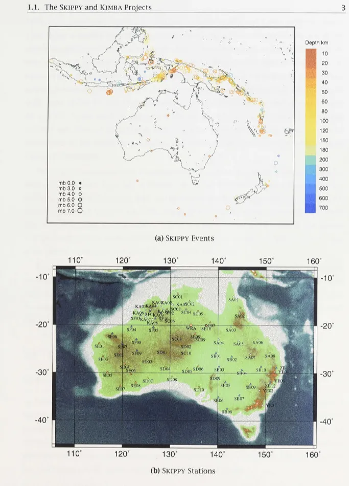
The SKIPPY project consists of 73 temporary broadband three-component seismic stations evenly distributed across the Australian continent to supplement the sparse network of per-manent broadband stations (Figure l.l(b)). Arrays of up to 12 stations have been deployed, covering the continent in 6 major deployments (stations SA-SF, Figure l.l(b)). The first array was deployed in northeastern Australia in May 1993. The last array, in far north Western Australia was completed in September 1996. The KIMBA project consists of a deployment of 10 closely spaced broadband stations in the Kimberley block deployed from July to October 1997 (Figure l.l(b)).

Recorders used in SKIPPY and KIMBA projects are Refraction Technology units with 24-bit

Analogue-to-Digital Conversion (ADC) and an internal Global Positioning System (GPS) cor-rected clock. Data are continuously recorded using a Digital Audio Tape (DAT) drive. The DAT drive was replaced by external disc drives for KIMBA and latter projects. The sensors in the field are three-component broadband Gfualp CMG-3ESP seismometers that are flat in ve-locity response from 30mHz to 30Hz. Four seismometers are flat to 0.016Hz (62.5 s period) (type 1) while the remaining eight are flat to 0.033 Hz (30 s period) (type 2). Data is digitised at 2 5 samples per second and with the flat velocity response of the sensors and 24-bit ADC ensures very high data quality. During the fifth and sixth deployments of the SKIPPY project (stations SE and SF, Figure l.l(b)) internal memory errors in the recorders have led to intermit-tent data loss. This has affected the analysis of surface waves for Western Australia and has also adversely affected the studies discussed here. Because of the poor data quality recorded at stations SE and SF, I have lost many paths in those area. However, I still have good path coverage in this area from data recorded at Warramunga and KIMBA stations.

Data are extracted for selected earthquakes (based on simple magnitude-distance criteria) from the Preliminary Determinations of Epicenters (PDE) catalogue, published by NEIC. Over

I.I. The SKIPPY and KIMBA Projects

f

'"\

t "~

'-0

mb 0.0 o 0

mb 3.0 o

mb 4.0 o mb 5.0 O mb 6.0 O

mb 7.0 0

11

o·

-1

o·

~

-20°

-30°

-40 °

~

..

I

.

\ ~

.

.. ". . ; I

-~ ' !_ , · -: '

---~~

..

d _. (' . a.

i

.

-'

.

\ oi

. c CIO, . , J , •

~

.

-

"

0 0 •

t}

~

ef

,;) C

0 ,

0

(a) SKIPPY Events

130° 140°

1so

fflf <>O

'l0<1 _<>·O

BG

BO

DOo SEO

OOll

BO

130° 140°

1so

(b) SKIPPY Stations

Depth km

l'.Jt;\1

ttf;

Vt'"' ,

-I

300 400 500 600 700 160° .JI

~I I -100

-20°

-30°

I

160°

Figure 1.1: (a) Events in the range of Mb 4.0-7.0 recorded at stations of the SKIPPY and KIMBA projects. When magnitude is not available, I mark it as Mb 0. (b) Portable and permanent stations used in _{this study. The six deployments} (SA-SF) of the SKIPPY project are shown as coloured triangles. The sta-tions of the KIMBA project are shown as white triangles. One permanent station (WRA array) is shown as red circle.

1.2. The Scope of the Thesis 4

2500 events have been archived for stations from the SKIPPY and KIMBA projects. Figure

l.l(a) shows a location map of earthquakes between Mb 4.0-7.0 recorded during the SKIPPY

and KIMBA projects and used in this study. The events occur mainly in the major earthquake

belt to the north and east of Australia, from Indonesia through to Fiji and New Zealand and to

a lesser extent from the east-Indian ridge, between Australia and Antarctica (fig l.l(a)). When

magnitude is not available I mark it as Mb 0. Seismicity falls into two general azimuth corridors to the north and to the east. Most seismicity to the east of Australia is concentrated between

30° and 50 °. To the north the majority of the seismicity is within 70 °. While the azimuthal

coverage and range of distances available limits the application of some techniques to the

SKIPPY data set the excellent data quality and station density allows us to investigate many

classes of information.

The KIMBA experiment used a concentration of instruments in northwestern Australia.

Stage one - K1MBA97: From July to October 1997 a set of broad-band instruments were

de-ployed in the Kimberley region, both on the King Leopold and Halls creek fold belt and the

interior of the block (Figure l.l(b)). This region of northern Australia has been the subject of

very little geophysical investigation on crustal and large scales, and the station placements

were designed to build on the information obtained from the stations in the SK3 and SK6 legs

of the SKIPPY experiment to improve knowledge of the region.

Stage two - KIMBA98: From May to October 1998 a set of 14 broad-band instruments

were deployed through the Kimberley region, crossing both the King Leopold and Halls Creek

fold belts and the interior of the block including the remote northern region (Figure 1.1 (b )).

The instruments deployed in 1998 (KB) were placed to improve the coverage from the 199 7

deployment (KA).

1.2 The Scope of the Thesis

Review of Previous Studies on Seismic Body Wave Attenuation

Seismic wave attenuation has been the subject of many studies in the last few decades. I

briefly review the progress in the determination of Q structure in the Earth both from

stud-ies of laboratory and seismological constraints on seismic wave attenuation. I focus on the physical mechanism of seismic wave attenuation, the frequency dependence of attenuation,

laboratory measurements on attenuatiop. and seismological constraints on 1-D Q profiles and

3-D Q structures in the upper mantle on global and local scales.

Numerical Simulation of Seismic Wavefield, Travel Time and t *

The upper mantle has a relatively complex structure. Beneath the continental areas the

1.2. The Scope of the Thesis 5

[Kennett, 1998]. There is usually a low velocity zone beneath the lithosphere and a rapid

increase in velocity with depth below 250km. Due to phase transition in the silicate minerals

of the mantle, there are noticeable jumps in seismic wavespeed near 410 and 660 km depth.

Those velocity discontinuities lead to triplications in the travel time curves for P and S and

produce complex seismic phases in the epicentral distance range from 15-28°.

In order to provide a background to understand and interpret the differential attenuation

measurement from SKIPPY data, I need to understand the seismic wave field in regional scale up to 50°. For this purpose, I have simulated the raypath distribution, travel time curve, slowness variation and t

*.

Theory and c5t* Measurement Techniques

I have developed a method to estimate the differential attenuation c5tJv based on the spectral ratio between P and S. I have investigated the effects of dispersion and frequency

dependence of attenuation. The wavespeed and Q both depend on frequency, but the effect

of dispersion is very small. Stable estimates of Q can be found for frequency less than 1 Hz.

For the broad frequency band up to 6Hz, Q is a function of frequency, latitude, longitude and

depth. In other words, Q is a 4-D parameter. The frequency parameter of Q is also dependent

on depth and position. I develop the techniques which allow us to estimate the c5tJv in a series of sub-frequency bands within a broad frequency band. Thus I am able to construct a 3-D frequency dependent Q model in chapter 9.

Measurement of the Path Average Properties of Attenuation

Although Q is a 4-D parameter of frequency and space, it is very difficult to model it in

4-D for a number of reasons. From Warramunga data I found that the differential attenu-ation between P and S show relatively constant low values at shorter epicentral distance, a steep increase for medium distances, and a gradual decrease at relatively large distance. The

differential attenuation variation with distance reveals the attenuation variation with depth.

From the work of Gudmundsson et al. [1994] and my successful experiments on Warramunga

and SKIPPY data, I found that I have good constraints on the measurement of c5 t iv over a nar-row frequency range near 1 Hz. The frequency dependence of attenuation may be significant

across a wide range of frequencies nevertheless its impact will be small across a narrow band. Based on the successful experiments on Warramunga and a few SKIPPY data, the SKIPPY data

set was analysed to determine the detailed attenuation structure in upper mantle under the

Australian continent.

To estimate the 8tJv from the SKIPPY data set, the P and S wave arrivals needed to measure

1.2. The Scope of the Thesis 6

average value of P and S velocity along the raypath. The estimation of P and S wave arrivals

reveals the lateral variation of the velocity along the whole path.

Then I systematically applied my approach of the measurement of spectral ratio in the

narrow frequency band to the SKIPPY data set. From the spectral ratios of P and S wave, a set of measurement of differential attenuation 8tfp from nearly 2,000 raypaths was obtained

which covers the upper part of the mantle beneath the Australian continent. The

measure-ments clearly delineate major variations in attenuation between the cratonic structures in the

central and western and the eastern part of Australia. To visually display the lateral variation

of attenuation, the raypaths were plotted with colour scaled by 8tfp• As a result, clear

geo-graphical variation in attenuation across the Australian continent was revealed. This result

was presented by the author at the 1999 IUGG meeting at Birmingham, UK.

In a broad frequency band, the attenuation is dependent on the frequency. The path average parameter of attenuation dependence on the frequency y was estimated from the spectral ratio. It is different from the 3-D attenuation frequency dependence parameter ex

which could be inverted from the frequency dependent 8tfp in chapter 9. The estimation of

y is also shown clear lateral variation.

Comparing the variations in velocity structure, 8 tip and y across the continent, it was found that they are correlated with each other quite well. In the area of high velocity, the

attenuation is weak and the attenuation dependence on frequency is also weak. Meanwhile,

the strong attenuation corresponds to the low velocity zone. Weak attenuation of S waves was

found in central and western Australia where the S velocity is high. But strong attenuation of

S waves was found in eastern Australia and Coral Sea area with low S wave velocity.

The correlation between attenuation, attenuation dependence on frequency and velocity

provides a good background for inverting a 3D attenuation model in the upper mantle.

3-D Attenuation Structure in the Upper Mantle

Based on the robust measurement of differential attenuation 8 tip in the narrow frequency

band below 1 Hz, I have constructed 3-D attenuation structure in the upper mantle beneath

the Australian continent. First I sorted my raypaths into a set of azimuth corridors at the

step of 20° from 0° to 80 ° clockwise and 0° to -80 ° anticlockwise. I have also divided every

corridor into 4 slices. I have undertaken inversion for Q from the estimates of 8 t ₅*P by using

a recently developed nonlinear inversio:p. method with neighbourhood algorithm [Sambridge,

1999a,b]. Thus a set of 1-D profiles of Q at fixed frequency around 1 Hz was obtained. The

1-D Q profile with azimuth O derived by nonlinear grid search was presented by the author at the 1999 IUGG meeting at Birmingham, UK.

I have derived a pseudo 3-D Q model by combining the set of 1-D Q profiles. First, I

1.2. The Scope of the Thesis 7

function represents the depth dependence of raypath density. Other two functions represents

the lateral variation of raypath density at certain depth. Then I undertook a grid search across the whole area within my data coverage. The grid search was undertaken layer by layer.

Because the slices from different azimuth corridors are overlapped, I obtained a Q value for each point by averaging the Q -1 _{values from the slices which cover the point weighted by}

three sets of raypath density functions of each slice which represents the raypath density

vary with vertival and lateral variation raypath density.

Numerical Simulation and Measurement of 8 t

iv

The 8tJv estimation from the SKIPPY data set at centre frequency of lHz reveals the lateral

variation of attenuation. The measurement of path average frequency dependence of

atten-uation reveal the depth dependence of frequency dependence of attenatten-uation. Temperature

dependence of frequency dependence of attenuation has been found in laboratory studies.

For better understanding the 8 t

Iv

iv

=

₀

=

at the lithosphere, corresponding to distances less than 16°. There are dramatic changes in

8tJv from 16° to 18°. The changes in 8tJv at this distance range contributed by the big jump

in velocity at 410 km discontinuity. The changes in 8 t

iv

and the asthenosphere.

3-D Frequency Dependent Attenuation Structure in the Upper Mantle

Because of raypath coverage and/or data limitations, all the previous studies on frequency

dependence of attenuation have focused on modeling the mean value of Q dependent on

frequency along a raypath. The quality and dense broadband SKIPPY data allows me to obtain

a set of measurements of 8 tip as a function of distance and frequency in a broad frequency

band up to 6 Hz. A set of 1-D profile of Q and ex were obtained by inversion using NA

from estimates of frequency dependent 8tJv with same parameterisation as I undertook the inversion for Q model at fixed frequency.

By using the same method when I derived the 3-D Q model at fixed frequency, I have

constructed the pseudo 3-D ex model tr1 the upper mantle which has not been done before.

Considering the error with 8tJp estimation, the Q derived from frequency dependent 8tJp is

consistent with Q model derived from 8tJv estimated at fixed frequency. My estimation of

3-D Q and ex reveal the spatial variation of the seismic body attenuation and its frequency

Chapter 2

Q

The attenuation structure of the upper mantle has been the subject of many studies in the last 30 years. Useful reviews on attenuation theory, observation techniques, and results have been given by Gordon and Nelson [1966], Anderson [1967], Sato [1967], Jackson and

Ander-son [1970], Smith [1972], Kennett [1975, 1983], Dziewonski [1979], Minster [1981], Priestley and Chavez [1985]; Chavez and Priestley [1986]; Priestley [1988], Anderson [1989], and more recently by Douglas [1992], Nakanishi [1993], Gudmundsson et al. [1994], Sharrock [1995]; Sharrock et al. [1995], Bahttacharyya et al. [1996], Roth et al. [1999], Romanowicz and Durek [2000]. The studies on seismic wave attenuation and scattering in shallow part of lithosphere, particularly in the crust has been thoroughly reviewed and summarised by Aki [1980a,b], John-ston and Toksoz [1981], Wu and Aki [1988b, 1989, 1990] and more recently by Sato and Feher [1998]. The recent progress on laboratory studies on seismic wave attenuation and attenu-ation mechanism was reviewed by Karato and Spetzler [1990]; Karato et al. [1995], Jackson [1991, 1993, 2000).

A special issue of Pure and Applied Geophysics in 1998 has included a variety of perspec-tives_ on Q. It includes papers pertaining to a dislocation model for seismic wave attenuation and creep [Karato, 1998); the state of global Q tomography [Romanowicz, 1998]; on tel~seis-mic body waves, both observational results [Der, 1998; Morozov et al., 1998) and methodology [Bahttacharyya, 1998; de Lorenzo, 1998]; and on subduction zones [Sato et al., 1998; Flana-gan and Wiens, 1998]. The issue also includes studies that cover a broad range of scales and distances. These include papers on laboratory studies of crustal rock [Lu and Jackson, 1998]; surface waves [Cong and Mitchell, 1998b]; and L₉ coda [Cong and Mitchell, 1998a; de Souza and Mitchell, 1998; Baqer and Mitchell, 1998; Mitchell and Cong, l 998a,b] over distances of 100 to 1000 or more km, on regional body waves [Sarker and Abers, 1998; Tselentis, 1998; Ugalde et al., 1998; Gupta et al., 1998], and local frequency dependent attenuation structure of P and S waves in the upper crust [Yoshimoto et al., 1998);

In this chapter, I summarise the definition of Q and review physical mechanisms and

2.1. Attenuation Terms and Definition of Q 9

laboratory measurements on seismic wave attenuation, the limitations and improvement of

seismological attenuation observation techniques and attenuation tomography.

2.1 Attenuation Terms and Definition of

Q

2.1.1 Definition of

Q

Real Earth materials are not perfectly elastic. Any anelastic processes will lead to the dissipation of seismic energy as seismic waves propagate through the Earth; in other words,

seismic waves attenuate or decay as they propagate. The anelastic behaviour can be included

in the constitutive law for the material by introducing the assumption that the stress at a

point depends on the time history of strain.

The most commonly used measures of attenuation found in the literature are the quality

factor Q and its inverse Q-1, which may be defined as:

Q-1 (j)

=

Here i6.E(f) is the energy loss in one cycle at frequency f, and Eo is the elastic energy stored in the oscillation. If I use the amplitude instead of energy in equation (2.1), then I get

Cl.A TT

A=

Considering the attenuation, the amplitude has to take the form

TT l

A ~ Ao exp ( - Q A. ) ,

TTf

- Ao exp(-Ql).

(2.2)

(2.3)

Other parameters used to measure attenuation are the attenuation coefficient y which is the exponential decay constant of the amplitude of a plane wave traveling in a homogeneous

medium, and the logarithmic decrement b. These quantities are related as follows [Johnston

and Toksoz, 1981]:

Q _ 1 = Imµ

=

Reµ TT f 8.686TT '

where:

Q

=

y

=

Reµ, Imµ= real and imaginary parts, respectively of complex modulusµ,

V

=

2.1. Attenuation Terms and Definition of Q 10

f = frequency.

The attenuation coefficient may be expressed in nepers/unit length (or simply inverse length)

or in dB/unit length. The relationship between the two is given by y(dB/unit length)= 8.686y

(nepers/unit length), and as noted in equation (2.12), y(dB/.\ = 8.686rr /Q.

The energy dissipation 8£ is just associated with the imaginary parts of the elastic moduli.

For purely dilational disturbances:

Q;

and for purely shear effects

Q·;/

For the Earth it appears that loss in pure dilatation is normally much less significant than loss

in shear, and then Q;-1 _<<

_Qi/

2.1.2 Intrinsic Attenuation and Scattering

Seismic attenuation is caused by either intrinsic anelasticity or scattering attenuation.

The is intrinsic anelasticity characterised by attenuation quality factor, Qin associated with

small-scale crystal dislocations, friction, and movement of interstitial fluids. The scattering

attenuation, associated with an elastic process of redistributing wave energy by reflection,

refraction, and conversion at irregularities in the medium, is often characterised by an

ex-ponential attenuation quality factor, Qsc• The latter process is not true anelasticity but has

virtually indistinguishable effects that are not accounted for by simple Earth models. Unlike

Q defined for anelastic processes, Qsc is not a measure of energy loss per cycle but, rather,

a measure of energy redistribution. Qsc depends very strongly on frequency and is very

path dependent, since it depends on the particular heterogeneity spectrum encountered by a wavefield propagating through the Earth. Qsc is usually modeled with stochastic operators,

or randomisation coefficients. According to Kennett [1983] and Richards and Menke [1983],

the scattering contribution to attenuation may be accounted for by

Q -1 _ob

₌

In order to separate the scattering effect from intrinsic attenuation, Wu and Aki [1985] de-veloped a multiple scattering model for seismic wave propagation in random heterogeneous

media. In their research, a radiative transfer theory was applied to seismic wave

propaga-tion and the energy density distribupropaga-tion in space for a point source was formulated in the

frequency domain. It is possible to separate the scattering effect and the absorption based

on the measured energy density distribution curves. By comparing the theory with data from

2.1. Attenuation Terms and Definition of Q 11

scattering is not the dominant factor for the measured apparent attenuation of S waves in the frequency range 2-20 Hz. From estimations at high frequency (j > 20 Hz), they suggest the existence of a strong-scattering surface layer with small scale heterogeneities in the crust, at

least for the Hindu Kush region which they studied [Wu and Aki, 1988a].

More recently, the P and S wave scattering was investigated by Tilmann et al. (1998] from mantle plumes. Sato and Feher (1998] thoroughly summarised the intrinsic attenuation

mech-anism and scattering for crustal propagation and discussed various mechmech-anism for intrinsic

attenuation and their frequency characteristics. They have also discussed the scattering of

seismic waves caused by random heterogeneities as a mechanism to explain the excitation

of incoherent S-coda waves. Taking scalar waves as an example, Sato and Feher [1998]

in-troduce an approach for calculating the amount of scattering attenuation in agreement with

conventional seismological attenuation measurements.

At frequencies with wavelengths much larger than the heterogeneities in the medium,

in-trinsic attenuation dominates; so that the energy loss through nonelastic processes is usually

measured by intrinsic attenuation and parameterised with Q. Large values of Q imply small

attenuation. In this research, I will focus on the intrinsic attenuation in the upper mantle.

2.1.3 Frequency Dependence of Intrinsic

Q

Because the real Earth is not perfectly elastic, propagating seismic waves will attenuate

with time due to various energy-loss mechanisms, such as movements along mineral

dislo-cations or shear heating at grain boundaries. Those processes are generally described as

internal friction and are difficult to model because the microscopic processes are complex.

The attenuation of seismic waves is commonly characterised by a Q value which is observed

to be largely independent of frequency in the range from 0.001 to l.0Hz, [see e.g. Sipkin and

Jordan, 1979]. At higher frequencies, Q depends on frequency and, in general, increases with

frequency.

An absorption band model is commonly used to explain both the absorption and

as-sociated dispersion of seismic waves in the mantle [Liu et al., 1976; Anderson and Given,

1982]. The behaviour of this mechanical model explains discrepancies between long- and

short-period seismic observations so that the apparently weaker damping observed for higher

frequency waves [e.g. Sipkin and Jordan, 1979] is likely to be a rheological property of mantle

materials.

Over the frequency band 0.001-10 Hz in seismological studies, the intrinsic loss factor

Qµ

loss mechanism,

Qµ

observed results confirm this conclusion, such as, Q for seismic waves is observed to be

2.1. Attenuation Terms and Definition of Q 12

frequency, Q depends on frequency and, in general, increases with frequency. To explain the

frequency dependence of QI follow the discussion by Kennett [1983]. In order to express the

macroscopic characteristics of the material within the Earth, a constitutive relation between

the stress and strain is needed. For linear elastic media, the stress field TiJ is related to the

displacement u by,

Tij = Cijk[O[Uk- (2.8)

with oi

=

a

Cijkl = C jikl = Cijlk = Cklij. (2.9)

On a fine scale the Earth material will have a relatively chaotic assemblage of crystal grains with

anisotropic elastic moduli. However, the overall properties of a cube with the dimensions of a

typical seismic wavelength (a few kilometres in the mantle) will generally be nearly isotropic.

In consequence the elastic constant tensor may often be approximated in terms of only the bulk modulus K and shear modulus µ

2 Cijkl

=

-3

The rheology of mineral assemblages is very complex in the crust and mantle. The

rheolog-ical behaviour depends on the time scale. Over geologrheolog-ical time scale they can sustain flow.

However, on the relatively short time scales appropriate to seismic wave propagation

(0.0ls-l000s), the behaviour will be nearly elastic with a modest influence of the long-term rheology.

The small incremental strains associated with seismic disturbances suggest that departures

from constitutive relations (2.8) should obey some linear law [Kennett, 1983].

The anelastic behaviour could be included in the constitutive laws by introducing the

assumption that the stress at a point depends on the time history of strain, so that the material

has a 'memory' [Kennett, 1983] . The theory of such linear viscoelasticity has been reviewed

by Hudson [1980]. The isotropic constitutive law which describes linear viscoelasticity is

[Hudson, 1980; Kennett, 1983]:

TiJ

=

+

J:

+

+

Here Ao

=

wave speeds and R11 , Rµ are relaxation functions specifying the dependence on the previous

strain states.

Taking the Fourier transform of (2.12) with respect to time, in terms of stress and

dis-placement at angular frequency w I get

2.1. Attenuation Terms and Definition of Q 13

where A_{1 and µ 1 are transforms of the relaxation terms:}

,\i(w) =

fooo

fooo

The form of the stress-strain relation at frequency w (2.12) is as for an elastic medium, but now with complex moduli.

Because the relaxation contribution to (2.9) depend only on the past history of the strain,

Rµ

(Imw > 0). In _{consequence the real and imaginary parts of µ 1 (} w) are the Hilbert transforms

of each other (see, for example Kennett, 1983; Titchmarsh, 1937]

Re{µ1(w)}

=

I_Pf

dw'Im{~i(w)},

TT -oo W - W

(2.14)

where P denotes the Cauchy principal value. From the definition of

Qi/,

frequency.

R { _{e µl} ( )}_W =_2µoplood ,w'Qµl(w') _{W ,2 2 .}

TT O W - W

(2.15)

When I wish to use observational information for the loss factor Qµ1 (w) I am faced with the difficulty that this only covers a limited range of frequencies, but the detailed form of

Re{µ 1 (w)} depends on the extrapolation of Qµ1 _{(w) to both high and low frequencies. If Qµ}1

is not too large, the approximate relation:

Re{µ1(w)} = 2µoln(taf)Q·;/!TT. (2.16)

for some time constant ta, fits a number of classes of model with approximately constant

Q-1 µ .

Kennett (1983] also developed the complex bulk modulus Ko + K_{1 (} w) in terms of the loss factor Q; 1. For a locally uniform region, at a frequency f, as in a perfectly elastic medium,

two sets of plane waves exist. The S waves have a complex wave speed

Vs

- 2

Vs (w)

=

influenced only by shear relaxation process. In terms of the wave speed Vso = (µ0 / p) 112

calculated for the instantaneous modulus, (2.17) may be rewritten as

- 2 ₂ Re{µ1(w)} . _{_1}

Vs (w) = Vs₀(1 + - - - 1sgn(w)Qµ (w), (2.18)

µo

when I have used the definition of Qµ1 in equation (2.6). Even if Qµ1 _{is frequency independent} in the seismic band, my previous discussion shows that

Vs

through Re{µ1 (w) }.

For a small loss factor (Qµ 1 << 1) the ratio of complex velocity at two different frequencies

f1 and f2 will from (2.18) be approximately

~s(W2) =l Qµlln(W1)_· ( )~Q-1( )

V ( s W1 ) + TT W2 1sgn w 2 µ w .

2.1. Attenuation Terms and Definition of Q 14

The problem of the unknown constant ta can be overcome by fixing a reference frequency

most commonly 1 Hz and then,

v's( w)

~

rr-1_{Q;/(w) ln(w / 2rr) - isgn(w)}

~

where V51 is the velocity at 1 Hz. The real part of this equation is the velocity dispersion

contributed by attenuation with the condition of Qi/ is independent of frequency [see also

Kanamori and Anderson, 1977].

When

Q-;;

dependence Re{V5 (w)} will vary. Under the condition of power low relationship between Q

and frequency as Q(j ) = Qofcx. and at reference frequency 1 Hz, the dispersion takes the form (2.21), (see also equation (2.36) and Jackson, 1993).

\ /5 ( w) "" V5o [ 1 - tan (( 1 - oc) TT / 2) ) QQ

1

u: ) "']

I simulated the effect of dispersion based on (2.21) in section (8.2.4). I found the effects of dispersion to be very small in general. The D tip calculated with dispersion are slightly smaller

than DtJP calculated without dispersion at smaller distances and lower frequencies . They are

identical at higher frequency and larger distance (see (8.2.4) for details ).

For P waves the situation is a little more complicated since anelastic effects in pure

di-latation and shear are both involved. The complex wave speed Vp is

- 2 4 1

Vp (w )

=

3µ o+ K1( w )+

3

- Vpo{l + A(w) + isgn(w )Q,;1 (w)}, (2 .22)

where

4

Vpo =[ (Ko+

3

and I have introduced the loss factor for the P waves.

1 4 4

Qp

3

The real dispersive correction to the wave speed A(w) will have a rather complex form in

general but under the conditions leading to a linear relationship between

Q;

is a similar form to (2 .16).

4

A(w)

=

+

3

and again for the complex wave speed has the form in terms of the wave speed at 1 Hz

Vp(w)

~

Q,;

J.

(2.2 5)

(2.26)

It is believed that intrinsic attenuation in the Earth mantle occurs almost entirely in shear

2.1. Attenuation Terms and Definition of Q 15

The above discussion can be simplified by introducing stress and strain relaxation times.

Following Lay and Wallace [1995], a standard linear solid can be used to explain and simplify

the above discussion of the frequency dependence of Q. For this model, the constitutive law

is written

a-+ TerO" = µo(E + TEE) (2.2 7)

where µo is called the relaxed elastic modulus, and T er and TE are called the stress and strain relaxation times, respectively. T er implies constant strain, and TE implies constant stress. Equation (2.2 7) is a special case of (2.12).

0-1

Mr

p

0.01

-~--c2 (W)

0.1 ,o 100

IDtcr

(a) Single Debye peak

M, -i:,

p "t

C1

Q1

10~ 10-4 10° 104

0.01 _...,.._.

\ I \ I \

\ I

,,

V

"

/\ I \ \

0.05 I \ I \ _\

I

,,

I _I\ \ _\

/ I

' '

'

'

.,, ....

{I)

(b) Superposition of Debye peaks

Figure 2.1: (a) Q-1 as a function of frequency for a standard linear solid. The peak in Q-1 is know as a Debye peak. (b) Superposition of numerous Debye peaks results in an absorption band-nearly constant Q over a range of frequencies. After Lay et al. 1995.

The behaviour of (2.27) can be investigated by looking at the ratio of harmonically

time-varying stress to strain:

a-(t) / E(t)

=

µ is called the complex elastic modulus and is given by

µ

=

and

s: ( w2Tt . WTer )

µc = u µ - - - = - + i =

-1 + w

2T&

2T&

where 6µ

=

=

2T2

w er

Reµc

=

T&

WTer

Imµc = 1 +

w2T&

(2.31)

(2.32)

This complex elastic modulus has several significant differences from simple elastic

2.1. Attenuation Terms and Definition of Q 16

This implies that waves traveling through such a solid will be dispersed. In other words, the different frequencies in a seismic wavelet will travel with different velocities. I can write the phase velocity as

V (w) =

~(1+~<5µ)

P

"yP

- fj

(1

~

This equation is valid only for small <5µ. Note that if <5µ = 0, the Vp is independent of

frequency and is, of course, just the velocity in the elastic case. For small <5 µ l can also write

an equation for Q:

Q-l(W)

=

WTo-µo 1 + w

2T&

<5µ

- -lmµc

µo (2.34)

When the above expressions are plotted as a function of WT a-, the behaviour of attenuation

versus frequency is shown in figure 2.l(a): intense attenuation occurs over a limited range of

frequencies centred the Debye peak. In general, each relaxation mechanism in the Earth has

a distinct Debye peak. These relaxation processes may involve grain boundary sliding, the

formation and movement of crystal lattice defects, and thermal currents.

Because of the great variety and scale of attenuation processes in the Earth, no single

mechanism dominates [Lay and Wallace, 1995]. The sum or superposition of numerous Debye

peaks for the various relation processes, each with a different frequency range, produces a

broad, flattened absorption band. Figure 2.l(b) shows the superposition effect. The Q-1 is basically constant for frequencies of LO Hz to 2.8 x 10-4 _{Hz [Lay and Wallace, 1995]. This is}

likely the reason why the observation of attenuation from seismic wave indicates that Q is

frequency independent over a large range of seismic frequencies. However, my estimation of

frequency dependent <5 tip in a broad frequency band up to 6 Hz allows me to invert Q and

ex as a function of depth at same time. Hence, both depth dependence of Q and the depth

dependence of frequency dependence of Q were obtained in thesis (see details in chapter 9).

2.1.4 Previous Seismological Studies on Frequency Dependence of Body

Wave Attenuation

The frequency dependence of Q has been investigated in the last few decades for regional,

teleseismic distances and global scale sampling of the crust and mantle by various authors

[Anderson and Minster, 1979; Sipkin and Jordan, 1979; Aki, 1980a,b; Clements, 1982; Der et al.,

1982, 1986; Roecker et al., 1982; Ulug and Berckhemer, 1984; Douglas, 1992; Bahttacharyya

et al., 1996; Flanagan and Wiens, 1998; Martynov et al., 1999].

Sipkin and Jordan [1979] investigated the frequency dependence of

Qscs

2.1. Attenuation Terms and Definition of Q 17 that Qscs is frequency dependent and takes the form of power law relationship between Qscs and frequency Qscs ex: fa with ex= 0.35 in the frequency range 0.0l-2Hz. Der et al.

[1982] investigated the regional variations and frequency dependence of anelastic attenuation in the mantle under the United Sates in the 0.5-4.0 Hz band. They found a large variation in the attenuative properties of the upper mantle under the United States. Their data indicate that attenuation is greatest under the south-western United States and the lowest attenuation prevails under the north central shield regions. They have found that the Q is frequency dependent and doubles in value somewhere in the range of 0.01-2.0Hz. They also indicated the form of frequency dependence may change from region to region, and the depth distribution of Q may be different at various frequencies. But these uncertainties can only be resolved by further detailed studies.

Ulug and Berckhemer [1984] summarised the range of studies on the frequency depen-dence of Q up to 1982. For a model with a power law dependence on frequency, Q (j ) = Q0f rx, the value of ex for the whole Earth is 0.2-0.4 in the frequency range 10-8 - 10-2Hz, for mantle,

ex is 0.15-0.6 in the frequency range 0.001 - 2.0Hz, for crust, ex is 0.25 - 1.0 in the frequency range 0.025 - 48 Hz. Laboratory data suggest ex is 0.25 - 0.3 in the range 10-4 - 30 Hz. Ulug

and Berckhemer [1984] also investigated the frequency dependence of attenuation of P and

S waves using 17 earthquakes at 40° - 90° range recorded at CSO, Germany and compared their results with previous investigations. They found their results are in good agreement with Sipkin and Jordan [1979]. Their Q model can probably best be represented by a power law absorption band Q ( j) = Qof cx with a slope of 0.2 5 < ex < 0.4 and a cut-off relaxation

time 0.2 < T < 0.5s. This model is of the type proposed by Anderson and Given [1982] for

absorption in the mantle.

A more thorough summary of values of ex and Qo in the shallow lithosphere estimated from short distance seismic waves was given by Sato and Feher [1998]. The frequency de-pendence of the attenuation in the form of a power law as Q_{5 ::::::} Q50f cx. for the frequency dependence higher than 1 Hz. Values of the exponent ex range from 0.2 to 1. Q5o is of the

order of 102 at 1 Hz and increase to the order of 103 at 20Hz. Based on the Q5 to be of 103

2.1. Attenuation Terms and Definition of Q 18

in the crust, in the case of scattering is dominant. For the long distance events which traverse

in the upper mantle, the Qp / Q5 ratio, should be only slightly affected by scattering. So that

the intrinsic attenuation is dominant in the upper mantle and the Qp I Q5 ratio will be around

2.25.

Flanagan and Wiens [1998] have summarised recent progress in attempting to quantify

the frequency dependence of attenuation in the upper mantle, they also investigated the

fre-quency dependent Q in upper mantle beneath Tonga region by a spectral-ratio method using

sS-S and pP-P pairs. The spectral ratio between sS-S and pP-P pairs allow them to estimate

the compressional wave attenuation Qo: and shear wave attenuation Q13 independently. Their

measurements suggest substantial frequency dependence of Qin the upper mantle beginning

at frequencies less than 1.0 Hz and consistent with the power law form: Q (j) = Qof o: with

ex between 0.1 and 0.3.

By using the Pg, Sg, and SmS body waves and S coda waves from analysing 243

three-component broadband digital seismograms of aftershocks from the M5 = 7.3 Suusamyr,

Kyrgyzstan earthquake, Martynov et al. [1999] investigated the high frequency (1.2-30 Hz)

attenuation in the crust and upper mantle of the Northern Tien Shan. By taking the power

law model Qj (j)

=

76 (upper crust) to 1072 (upper mantle), and the value of ex J decrease from 0.99 to 0.29 over

the same range. The Q coda results also demonstrated an azimuthal dependence. There is a

strong

2cp

dependence of the quality factor show that Q is complicated and three dimensional. They

also indicated that the lateral variation of Q0 can be connected with azimuthal anisotropy in

the upper mantle related to current deformation under the Tien Shan.

Multiple-frequency bands techniques similar to those I have developed in chapter 9 were

reported in the AGU 2000 spring meeting by Mamada and Takenaka [2000]. Mamada et

al. [2000] studied the S -wave attenuation in the focal regional of the 1997 northwestern

Kagoshima earthquake, Japan. They used the coda normalisation method to estimate Q

₅

dependence of Q5 is Q

5

=

5

=

crust of the whole western Kyushu including the focal area they studied. Mamada et al.

ex-plain the main reason for this extremely low Q is due to the focal region fractured completely with mainshock and a large number of aftershocks (personal communication). They did not