Generalised linear models for flexible parametric modelling of the hazard function

White Rose Research Online URL for this paper:

http://eprints.whiterose.ac.uk/149591/

Version: Accepted Version

Article:

Kearns, Benjamin, Stevenson, Matt, Triantafyllopoulos, Kostas et al. (1 more author)

(Accepted: 2019) Generalised linear models for flexible parametric modelling of the hazard

function. Medical Decision Making. ISSN 0272-989X (In Press)

[email protected] https://eprints.whiterose.ac.uk/

Reuse

Items deposited in White Rose Research Online are protected by copyright, with all rights reserved unless indicated otherwise. They may be downloaded and/or printed for private study, or other acts as permitted by national copyright laws. The publisher or other rights holders may allow further reproduction and re-use of the full text version. This is indicated by the licence information on the White Rose Research Online record for the item.

Takedown

If you consider content in White Rose Research Online to be in breach of UK law, please notify us by

flexible parametric modelling of

the hazard function

Reprints and permission:

sagepub.co.uk/journalsPermissions.nav DOI: 10.1177/ToBeAssigned www.sagepub.com/

SAGE

Benjamin Kearns (MSc)

_{, Matt Stevenson (PhD)}

_{, Kostas}

Triantafyllopoulos (PhD)

_{, and Andrea Manca (PhD)}

Abstract

Background:Parametric modelling of survival data is important and reimbursement decisions may depend on the selected distribution. Accurate predictions require sufficiently flexible models to describe adequately the temporal evolution of the hazard function. A rich class of models is available among the framework of generalised linear models (GLMs) and its extensions, but these models are rarely applied to survival data. This manuscript describes the theoretical properties of these more flexible models, and compares their performance to standard survival models in a reproducible case-study.

Methods:We describe how survival data may be analysed with GLMs and its extensions: fractional polynomials, spline models, generalised additive models, generalised linear mixed (frailty) models and dynamic survival models. For each, we provide a comparison of the strengths and limitations of these approaches. For the case-study we compare within-sample fit, the plausibility of extrapolations and extrapolation performance based on data-splitting.

Results:Viewing standard survival models as GLMs shows that many impose a restrictive assumption of linearity. For the case-study, GLMs provided better within-sample fit and more plausible extrapolations. However, they did not improve extrapolation performance. We also provide guidance to aid in choosing between the different approaches based on GLMs and its extensions.

Conclusions:The use of GLMs for parametric survival analysis can out-perform standard parametric survival models, although the improvements were modest in our case-study. This approach is currently seldom used. We provide guidance on both implementing these models and choosing between them. The reproducible case-study will help to increase uptake of these models.

Keywords

1

Introduction

In many medical studies the outcome of interest is the time until an event occurs. Examples include mortality, disease progression, or hospital admission. To aid with decision-making the hazard function is estimated from parametric models. A prominent example is health technology assessment (HTA), which aims to quantify both the benefits to patients and the costs a healthcare system would occur if a treatment were funded [1]. To allow for fair comparisons across different treatments it is important that all relevant benefits and costs are quantified, which often requires use of a lifetime horizon [2]. However, time-to-event (TTE) data with complete follow-up are rarely available. As such, parametric models may be used to extrapolate model-outcomes to a lifetime, and hence obtain estimates of mean TTE (such as mean survival) [3, 4].

Standard one and two parameter models are available, including the exponential, Weibull, Gompertz, log-logistic and lognormal [5]. However, these models may not be sufficiently flexible to capture complex, time-varying hazards [6, 7]. In Section 2 we introduce generalised linear models (GLMs) and show that standard survival models may be expressed as GLMs. This provides insight into the limitations of the standard models: they all impose an assumption of linearity. More flexible parametric models that relax this assumption are required. A number of these have been proposed within the framework of GLMs and its extensions, but to-date they are seldom used to analyse TTE. These are described in Sections 3 and 4, with an overview in Section 5. An application of these is described in in Section 6, which demonstrates that the GLM-based models can provide superior within-sample estimates and more plausible extrapolations than standard survival models. Concluding remarks are provided in Section 7.

This manuscript has two aims. The first is to propose the use of GLMs for the analysis of TTE data. This includes flexible GLMs such as fractional polynomials (FPs) and restricted cubic splines (RCS), which are closely related to Royston-Parmar (R-P) models. The second aim is to present generalisations to GLMs: generalised linear mixed models (GLMMs) [8], generalised additive models (GAMs) [9] and dynamic generalised linear models (DGLMs) [10, 11].

2

Analysing time-to-event data within a generalised linear modelling

framework

2.1

Standard survival models as linear models

The framework of GLMs extends (generalises) the standard linear model to response variables with distributions in the exponential family, including Normal, Poisson, Binomial, Gamma and

1_{The University of Sheffield} 2_{The University of York}

Corresponding author:

Inverse Gaussian distributions [12]. An advantage of GLMs is that they provide a unified framework - both theoretical and conceptual - for the analysis of many problems, including

linear, logistic and Poisson regression [13]. A random variable Y belongs to the exponential

family of distributions if its probability density (or mass) function can be written as:

f(yt;θ) = exp[a(y)b(θ) +c(θ) +d(y)] (1)

wherea(y) andd(y) are functions of the data, whilstb(θ) andc(θ) are functions of the distribution

parameter θ and assumed to be twice differentiable. Equation (1) may also include other

parameters, which are treated as nuisance parameters [13]. Examples for the Normal, Poisson

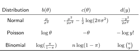
and Binomial distributions are provided in Table 1. For these,a(y) =y.

Table 1. Normal, Poisson and Binomial distributions as members of the exponential family

Distribution b(θ) c(θ) d(y)

Normal µ

σ2 -µ2

2σ2−

1

2log(2πσ

2₎ −y2

2σ2

Poisson logθ −θ −logy!

Binomial log( π

1−π) nlog(1−π) log n y

µandσ2are a mean and variance,πis a probability,nthe

number of trials and n y

=_y!(nn!

−y)! is the binomial coefficient.

For a TTE GLM, the observed outcome is the number of deaths during an interval:yt. This

is linked to the at-risk population at time t (denoted by τt) using a distribution from the

exponential family. Use of the Poisson distribution assumes that yt=τt×λt where λt is the

hazard at timet. Alternatively, use of the Binomial distribution assumes thatyt=τ1×ptwhere

ptis the cumulative probability of death. Model specification is [12]:

Observation model:E[yt] =µt×τt, yt∼exponential family distribution (2a)

Response function:µt=h(xTtβ) (2b)

whereE[·] denotes the expected value, bold font denotes a vector, and:

β is a vector of parameter coefficients to be estimated from the data,

xtis a covariate, assumed known (with transposexTt), and

h() is a one-to-one response function which maps the linear predictor (xT

tβt) to µt. Its

inverse is known as the link function, and is denoted asg().

Model parameters may be obtained via maximum likelihood estimation. The general expression for the logarithm of the likelihood is:

logL=

N

X

t=1

Lt=

N

X

t=1

ytb(θt) + N

X

t=1

c(θt) + N

X

i=t

WhereN is the number of time-intervals. For the Poisson and Binomial models, this becomes:

Poisson: logL=

N

X

t=1

[ytlog(θt)−θt−log(yt!)] (3a)

Binomial: logL=

N

X

t=1

ytlog

πt

1−πt

+ntlog(1−πt) + log

nt

yt

(3b)

In summary, a GLM may be specified by three components:

1. The distribution from the exponential family, as defined in equation (1),

2. the response (or link) function, and

3. the covariate vector.

For survival analyses, options forµtinclude the (cumulative) survival function, its complement

the (cumulative) failure function, the hazard function, and the cumulative hazard function - see [5, 14] for more details. Depending on the specification, we can express standard survival models

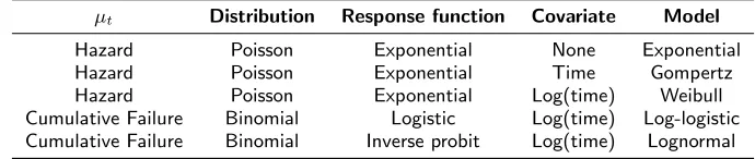
as a linear model: µt=β0+β1x_t. Table 2 provides these specifications. The log-logistic and

lognormal distributions have a cumulative function as their outcome. It would not be sensible to model such an outcome as a constant value which demonstrates why there is no single-parameter special case of these models. In contrast, the Weibull and Gompertz distributions model a non-cumulative outcome, so it is possible to model this as a single value, resulting in the exponential model.

Table 2. Specification of standard survival models as generalised linear models

µt Distribution Response function Covariate Model

Hazard Poisson Exponential None Exponential

Hazard Poisson Exponential Time Gompertz

Hazard Poisson Exponential Log(time) Weibull

Cumulative Failure Binomial Logistic Log(time) Log-logistic

Cumulative Failure Binomial Inverse probit Log(time) Lognormal

2.2

Limitations with linearity

The assumption of linearity may not always be realistic. For example, for overall survival the hazard of all-cause mortality will increase over time due to patient ageing. In contrast, frailty effects may result in disease-specific mortality decreasing over time (as those with an increased hazard will die sooner, leaving those with a lower hazard). The impact of treatment on survival may also vary over time: there may be an initial elevated risk of death due to adverse events; treatment-related toxicities may increase other-cause mortality over time, treatment stopping rules and trial inclusion criteria may have an effect [15]. These considerations motivate the need for more flexible survival models, which are considered within the GLM framework in the next two Sections.

3

Relaxing the assumption of linearity

We briefly describe flexible models that may be applied to survival data within a GLM

framework, more details are provided in the Appendix. Without loss of generality, y is used

to denote either a random variable or the observed data.

3.1

Fractional polynomials

FPs represent the outcome as a sum of polynomial terms; increasing the number of terms (the order of the FP) increases the flexibility of the model. A closed-test procedure may be used to

identify the order. For a single variable, anith

order FP is defined as:

E(yt) = FP(i) =β0+

i

X

j=1

βjxpj (4)

where the set of powerspj is pre-specified, and may include fractional powers (hence the name

fractional polynomials). FPs include linear models as special cases, so depending on specification may include one of the standard models from Table 2. Some limitations with FPs are that they may not have sufficient power to detect non-linearity, and they can be sensitive to extreme values

in the data. This sensitivity occurs because FPs areglobal models:β values are assumed to be

constant over time.

3.2

Restricted cubic splines and Royston-Parmar models

A cubic spline represents a continuous function as a series of piecewise cubic polynomials [14], hence relaxing the assumption of global time effects. Model flexibility is based on the number of piecewise intervals (equivalently, the number of ‘knots’). For extrapolation, the cubic polynomial from the last interval may be used, or it may be restricted to a linear function: this latter assumption results in an RCS. An example specification is provided in the Appendix.

R-P models use RCSs, but not in the GLM framework. Typically the outcome is the log cumulative hazard, which is monotonic. However, model estimates are not guaranteed to be monotonic, so implausible values may result.

4

Extensions to the generalised linear model

This section provides a brief overview of extensions to GLMs, with more details in the Appendix.

4.1

Generalised linear mixed models

A GLMM extends the GLM by incorporating random effect terms, which can help to quantify the impact of unmeasured covariates and provide more realistic estimates of uncertainty. An

example of an FP(2) with a random-effect (denoted bybt) is:

E(yt) = FP(2) =β0+bt+β1xp1+β2xp2, bt∼N(0, ψ

2

)

GLMMs are also referred to asfrailtymodels [17]. In theory, any GLM may be extended by adding

a random term as shown above. The main limitation with GLMMs is that as the random effects are not observed, there may be difficulties in model specification and parameter estimation.

4.2

Generalised additive models

A GAM is a GLM in which one or more of the covariates are modelled as a set ofbasis functions

[18]. For example, a univariate GAM is defined as:

E(yt) =

q

X

j=i

bj(t)βj=f(t)

Wherebj(t) is thejth basis function, andqis the dimension of the basis function. Higher values

of q result in more flexible models. Both FPs and RCSs may be viewed as GAMs. The main

extension provided by a GAM is that model complexity is penalised during parameter estimation

(via shrinkage of theβ). GAMs with a cubic spline basis have theoretical justification as being

approximate ‘smoothest interpolators’ [9] - see the Appendix for more details. Limitations of GAMs will depend on the basis function used. For example, if a spline is used, the limitations of these will still apply.

4.3

Dynamic generalised linear models and dynamic survival models

In a DGLM model coefficients (β) are allowed to vary over time. When applied to TTE data,

DGLMs are known as dynamic survival models (DSMs) [19]. Specification is (compare with

Equation 2a):

Observation model:E[yt] =µt×τt yt∼exponential family distribution (5a)

Response function: µt=h(xTtβt) (5b)

Transition model:βt=Fβt−1+ζt (5c)

Initial conditions:β0∼M V N(b0,Z0) (5d)

where M V N denotes a multivariate Normal distribution, F is a function describing how the

coefficients evolve over time, and ζt is an error term - see the Appendix for further details.

estimates may be based on minimising the error of within-sample extrapolations. This makes these models particularly appealing when the primary objective of the analysis is extrapolation. The main limitations with DGLMs are identifying suitable initial values, and convergence of algorithms to estimate model coefficients [20, 19].

5

Theoretical comparison of approaches

Five different modelling approaches were considered: FPs, splines, GAMs, GLMMs, and DGLMs. The frailty terms from a GLMM may be combined with either of the other four models. The following prompts are provided to aid with choosing between the different approaches.

What is the primary objective of the analysis? If the main objective is in generating

extrapolations, this implies the use of a DGLM, as this is the only one of the models for which parameter estimation is based on minimising forecasting error. If instead the main objective is to provide estimates of the observed data, then any of the approaches may be used.

Fractional polynomials or spline-based models? Spline-based models may be preferred

on theoretical grounds, as being approximate smoothest interpolators, whilst there are a number of limitations with the use of FPs (see the Appendix). This suggests the use of a spline-based model in preference to an FP within a GLM framework, with the latter as a form of sensitivity analysis.

To penalize during or after estimation? Parameter estimation with a GAM automatically

penalises for model complexity, which helps to avoid over-fitting. Alternatively, information criteria may be used. There are a number of different information criteria that could be used, whereas GAMs have a specific objective function. The choice between these is likely to be study specific: sometimes there may be good reasons to use a specific information criteria, whilst in others the more automated approach of a GAM may be preferred. For both approaches it is not possible to use significance tests to choose between model specifications.

Are there any subject matter considerations? For example, there may be reason to

believe that there are important unmeasured confounders, which suggests incorporating random effects. Or it may be thought that there will be important local fluctuations in this hazard, which suggests the use of either a spline or dynamic model in preference to the global FPs.

6

Empirical comparison of approaches

6.1

Dataset

We use a freely available dataset to demonstrate both the limitations of assuming linearity and

the use of more flexible models. Analyses were performed in R; the code used is available as

supplemental material. Hence the case-study is fully reproducible.

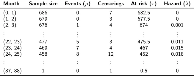
study conducted by the German Breast Cancer Study Group [21, 22]. Individuals with primary node positive breast cancer were recruited between July 1984 and December 1989. Events are defined as either death (from any cause) or cancer recurrence. Data are available for 686 individuals, of which 299 experienced an event during follow-up. The maximum follow-up was 7.28 years, with mean follow-up of 3.08 years. Use of GLMs requires that individual-level data are restructured in the form of life tables. Samples of the individual-level data and the corresponding (monthly) life table are provided in Tables 3 and 4, respectively. For Table 3, an event indicator of one denotes that an event occurred (otherwise the indicator is zero, and the outcome is time to censoring).

Table 3. A sample of the breast cancer data

Patient ID Outcome time (years) Event indicator

1 0.0219 0

..

. ... ...

15 0.1973 1

..

. ... ...

220 1.9562 1

221 1.9644 0

..

. ... ...

678 6.7288 1

..

. ... ...

686 7.2849 0

Table 4. Data from Table 3 restructured for Poisson regression

Month Sample size Events (µ) Censorings At risk (τ) Hazard (λ)

(0, 1) 686 0 7 682.5 0

(1, 2) 679 0 3 677.5 0

(2, 3) 676 1 4 674 0.001

..

. ... ... ... ... ...

(22, 23) 477 5 3 475.5 0.011

(23, 24) 469 7 4 467 0.015

(24, 25) 458 8 12 452 0.018

..

. ... ... ... ... ...

(87, 88) 1 0 1 0.5 0

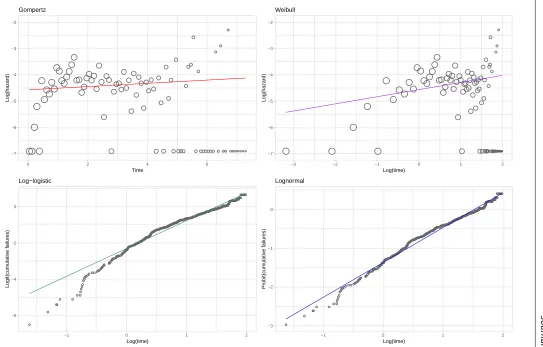
it would only be appropriate if both the Weibull and Gompertz estimates had no slope). The

specification of thexandy axis is such that the model estimates form a straight-line. Figure 1

Jou rn al T itl e X X (X ●● ● ● ● ● ● ●_●●● ●_● ●_●● ●● ● ●● ●● ●●_●● ● ● ● ● ●_● ● ● ●● ● ● ● ● ● ● ● ● ● ● ● ● ● ● ● ● ● ● ● ● ● ● ● ●●● ● ●● ● ● ● ●●●●●● ● ● ● ●● ● ● ● ● ● ● ●● −7 −6 −5 −4 −3 −2

0 2 4 6

Time Log(hazard) Gompertz ● ● ● ● ● ● ●●● ● ● ●● ●●● ●● ● ●● ●● ●●_●● ● ● ● ● ●_● ● ● ●● ● ● ● ● ● ● ● ● ● ● ● ● ● ● ● ● ● ● ● ● ● ● ● ●●● ● ●● ● ● ● ●●●●●● ● ● ● ●● ● ● ●●●●●● −7 −6 −5 −4 −3 −2

−3 −2 −1 0 1 2

Log(time) Log(hazard) Weibull ● ● ● ● ● ● ● ● ● ●● ● ●●● ●●●●● ● ● ●●●●● ●●●●●●●●●●●●● ●●●●●●●●●●●● ●●●●●●●●●●●●●●●●●●●●●●●●●●●●●●●●●●●●●●●●●●●●●●●●●●●●●●●●●●●●●●●●●●●●●●●●●●●●●●●●●●●●●●●●●●●●●●●●●●●●●●●●●●●●●●●●●●●●●●●●●●●●●●●●●●●●●●●●●●●●●●●●●●●●●●●●●●●●●●●●●●●●●●●●●●●●●●●●●●●●●●●●●●●●●●●●●●●●●●●●●●●●●●●●●●●●●●●●●●●●●●●●●●●●●●●●●●●●●●●●●●●●●●●●●●●●●●●●●●●●●●●●●●●●●●●●●●●●●●●●●●●●●●●●●●●●●●●●●●●●●●●●●●●●●●●●●●●●●●●●●●●●●●●●●●●●●●●●●●●●●●●●●●●●●●●●●●●●●●●●●●●●●●●●●●●●●●●●●●●●●●●●●●●●●●●●●●●●●●●●●●●●●●●●●●●●●●●●●●●●●●●●●●●●●●●●●●●●●●●●●●●●●●●●●●●●●●●●●●●●●●●●●●●●●●●●●●●●●●●●●●●●●●●●●●●●●●●●●●●● ●●●●●●●●● −6 −4 −2 0

−1 0 1 2

Log(time) Logit(cum ulativ e f ailures) Log−logistic ● ● ●● ● ● ● ●● ●● ● ●●●●●●● ● ● ●●●●●● ●●●● ●●●●●●●●● ●●●●●●●●●●●●● ●●●●●●●●●●●●●●●●●●●●●●●●●●●●●●●●●●●●●●●●●●●●●●●●●●●●●●●●●●●●●●●●●●●●●●●●●●●●●●●●●●●●●●●●●●●●●●●●●●●●●●●●●●●●●●●●●●●●●●●●●●●●●●●●●●●●●●●●●●●●●●●●●●●●●●●●●●●●●●●●●●●●●●●●●●●●●●●●●●●●●●●●●●●●●●●●●●●●●●●●●●●●●●●●●●●●●●●●●●●●●●●●●●●●●●●●●●●●●●●●●●●●●●●●●●●●●●●●●●●●●●●●●●●●●●●●●●●●●●●●●●●●●●●●●●●●●●●●●●●●●●●●●●●●●●●●●●●●●●●●●●●●●●●●●●●●●●●●●●●●●●●●●●●●●●●●●●●●●●●●●●●●●●●●●●●●●●●●●●●●●●●●●●●●●●●●●●●●●●●●●●●●●●●●●●●●●●●●●●●●●●●●●●●●●●●●●●●●●●●●●●●●●●●●●●●●●●●●●●●●●●●●●●●●●●●●●●●●●●●●●●●●●●●●●●●●● ● ● ●●●● ● ●●●●●●●● −3 −2 −1 0

−1 0 1 2

6.2

Methods

We considered five broad classes of model:

FP models. We considered FP(2) models, with the complexity of the chosen model based on

the closed-test procedure, and the chosen powers based on minimising AIC.

Generalised linear mixed models. We fit FP models as described above, but we also

included frailty terms.

Spline-based models. Both RCS models and GAMs were considered. For the RCS model

between 1 and 5 internal knots were considered, with the choice based on minimising AIC. For the GAM we considered two approaches to selecting the dimension of the basis function: one used a fixed (arbitrary) value of 11 (v1), the other was based on minimising AIC (v2). These two approaches were considered as some penalisation for over-fitting is included during model-fitting, so it is unclear if model choice based on AIC is required. For all models, the knots were placed at equally-spaced percentiles of the observed uncensored death times [21].

Dynamic models. We examined three specifications: local-level, local-trend, and local-level

with global trend. There was no need to base model choice on minimising AIC (as the data used to estimate the model parameters are separate to the objective function, which is based on minimising one-step ahead forecasts).

Standard survival models. Eight survival models were considered: exponential, Weibull,

Gompertz, gamma, log-logistic, lognormal, generalised gamma, and generalised F. Results are displayed for the three best fitting models (based on AIC). Note that the generalised gamma and generalised F models have three and four parameters respectively, so are more flexible than the standard survival models of Table 2.

The above choice of models was designed to be representative of the variety of different approaches possible, but not exhaustive. All of the models used the natural logarithm of time as the only covariate of interest (with the exception of the Gompertz, which uses time). All of the GLM-models assumed a Poisson distribution with an exponential response function.

6.3

Goodness of fit

Goodness of fit (GoF) measures how well the statistical model describes the observed data. It should be distinguished from predictive ability, which measures how well the model predicts external data (such as future observations). One measure of GoF is Akaike’s information criterion (AIC), which is defined as:

−2 logL+ 2k (6)

where Lis the model likelihood and kis the number of parameters in the model [23]. Because

Burnham and Anderson note that the AIC has strong theoretical motivation [23], whilst Jackson and colleagues note that the AIC is preferable when models are used to represent complex phenomena (such as survival processes) [25]. Due to having both empirical and theoretical support, the AIC shall be used in this manuscript. Any GoF measure should be used in combination with subject-matter considerations. In addition, estimates of the hazard function were visually compared to the observed hazard function.

The AIC measures GoF to the observed data. It is unknown if models with a good within-sample fit provide good extrapolations [14]. To measure the extrapolation performance of the models we split the dataset into two parts. The first part considered events occurring within the first three years, censoring all events after three years (half of the sample were at-risk of an event at three years). Extrapolation performance was defined as the sum of squared errors (SSE) between the model-estimate of the hazard and the observed hazard (calculated for monthly intervals) for the remaining follow-up:

ˆ λt−λt

2

, t∈ {37 to 88 months} (7)

6.4

Results

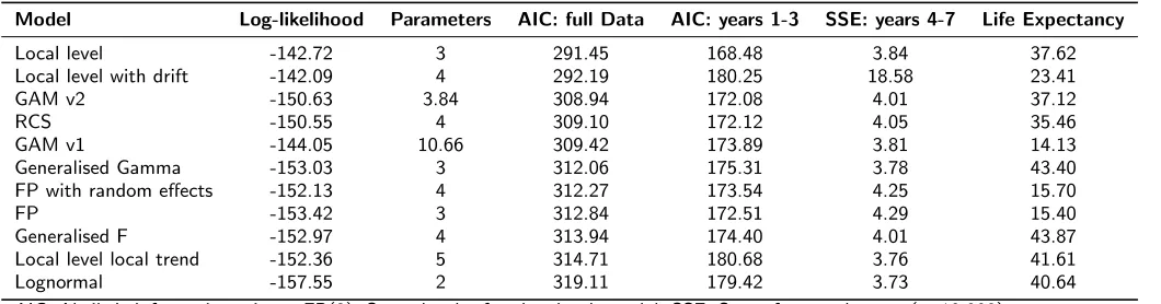
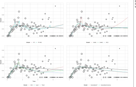
Table 5 provides GoF values for each model and estimates of lifetime mean life expectancy. Two AIC values are provided: one using the entire dataset, the other using the first three years. The number of parameters is provided as a measure of model complexity: the two GAMs do not have an integer number of parameters, as parameter effects are shrunk during model estimation. Plots of the estimated hazard function for each model are displayed in Figure 2 for the observed data. Corresponding extrapolations are given in Figure 3. As the best-fitting two-parameter standard survival model (based on all the available data), the lognormal is provided as a black reference line on all panes.

6.4.1 Within-sample goodness of fit All of the more flexible models provide lower AIC values than the lognormal, although in general differences between values are small, and cannot be tested for statistical significance. Visually, all of the models provide a good fit to the observed data in Figure 2, although there is variation in the degree to which local fluctuations are captured. Of the 11 models, the lowest AIC values arose from two DSMs. However, the third DSM had the highest AIC of all the flexible models. This suggests that the extension to dynamic models can lead to an improved GoF, but there is no guarantee that this will always occur. The next best AIC values arose from the three spline-based models, which all had very similar GoF. However, the two approaches to GAM estimation did result in markedly different models: the one with automated fitting was more complex (with almost three times as many parameters) than the one based on minimising AIC, whilst also providing a better absolute fit (based on log-likelihood). Of the three standard survival models, the two generalised models (gamma and F) both provided similar GoF, and both improved on the two-parameter models. Fit for the two FPs was similar to that for the generalised gamma and generalised F survival models, and lower than that for the spline-models. The inclusion of random effects had a negligible impact on the AIC.

This is most notable at approximately 1 and 1.5 years. However, as the most flexible models considered, there is a danger that these local fluctuations represent noise. If this is the case then the best-fitting models may be over-fitting the data, with no guarantee that this will lead to improved extrapolations.

6.4.2 Extrapolation goodness of fit When fitting the 11 models to the first three years, the ranking of the models was generally the same as for the full dataset, with the local level model providing the lowest AIC, and the lognormal one of the highest. An exception is the DSM with drift, which changes from having the second lowest AIC to the second highest. GoF to the observed data did not predict extrapolation performance. For example, the lognormal and local trend models both had the highest AIC values but the lowest SSEs. As with the AIC values, in general there was little difference between SSE values. An exception is the DSM with a drift, which provided poor extrapolations as it predicted an increasing trend.

Jou

rn

al

T

itl

e

X

X

(X

Model Log-likelihood Parameters AIC: full Data AIC: years 1-3 SSE: years 4-7 Life Expectancy

Local level -142.72 3 291.45 168.48 3.84 37.62

Local level with drift -142.09 4 292.19 180.25 18.58 23.41

GAM v2 -150.63 3.84 308.94 172.08 4.01 37.12

RCS -150.55 4 309.10 172.12 4.05 35.46

GAM v1 -144.05 10.66 309.42 173.89 3.81 14.13

Generalised Gamma -153.03 3 312.06 175.31 3.78 43.40

FP with random effects -152.13 4 312.27 173.54 4.25 15.70

FP -153.42 3 312.84 172.51 4.29 15.40

Generalised F -152.97 4 313.94 174.40 4.01 43.87

Local level local trend -152.36 5 314.71 180.68 3.76 41.61

Lognormal -157.55 2 319.11 179.42 3.73 40.64

AIC: Akaike’s information critera. FP(2): Second-order fractional polynomial. SSE: Sum of squared errors (×10,000)

For derivation of SSE values see section 6.3

re

d

u

si

n

g

sa

g

e

j.c

s et al ●●● ● ● ● ● ●_● ● ● ● ● ●_●● ● ● ● ●● ●● ● ● ● ● ● ● ● ● ● ● ● ● ●● ● ● ● ● ● ● ● ● ● ● ● ● ● ● ● ● ● ● ● ● ● ● ● ●●● ● ● ● ● ● ●●●●●● ● ● ● ●● ● ● ● ● ●● 0.00 0.01 0.02 0.03 0.04 Hazard

Model FP FP+RE

●●● ● ● ● ● ●_● ● ● ● ● ●_●● ● ● ● ●● ●● ● ● ● ● ● ● ● ● ● ● ● ● ●● ● ● ● ● ● ● ● ● ● ● ● ● ● ● ● ● ● ● ● ● ● ● ● ●●● ● ● ● ● ● ●●●●●● ● ● ● ●● ● ● ● ● ●●

Model GAM1 GAM2 RCS

●●● ● ● ● ●●● ● ● ● ● ●_●● ● ● ● ●● ●● ●●_●● ● ● ● ● ● ● ● ● ●● ● ● ● ● ● ● ● ● ● ● ● ● ● ● ● ● ● ● ● ● ● ● ● ●●● ● ● ● ● ● ●●●●●● ● ● ● ●● ● ● ● ● ●● 0.00 0.01 0.02 0.03 0.04

0 2 4 6

Time

Hazard

Model Drift Level Trend

●●● ● ● ● ●●● ● ● ● ● ●_●● ● ● ● ●● ●● ●●_●● ● ● ● ● ● ● ● ● ●● ● ● ● ● ● ● ● ● ● ● ● ● ● ● ● ● ● ● ● ● ● ● ● ●●● ● ● ● ● ● ●●●●●● ● ● ● ●● ● ● ● ● ●●

0 2 4 6

Model Generalised F Generalised Gamma

FP: fractional polynomial. RE: random effects. RCS: restricted cubic spline. GAM: generalised additive model. Gen: generalised. Hollow circles represent observed data; sizes are proportional to the denominator. For all panes the lognormal is included in

Jou rn al T itl e X X (X ●●●●● ● ●●●●● ●_● ●●●● ●● ●● ●●● ●_●● ● ● ● ● ●_● ● ●●●● ● ●● ● ● ● ●_● ● ●_●● ● ● ● ● ● ● ● ● ● ● ●●● ● ●● ● ● ● ●●●●●● ● ● ● ●● ● ●●●●●●● 0.00 0.05 0.10 0.15 Hazard

Model FP FP+RE

●●●●● ● ●●●●● ●_● ●●●● ●● ●● ●●● ●_●● ● ● ● ● ●_● ● ●●●● ● ●● ● ● ● ●_● ● ●_●● ● ● ● ● ● ● ● ● ● ● ●●● ● ●● ● ● ● ●●●●●● ● ● ● ●● ● ●●●●●●●

Model GAM1 GAM2 RCS

●●●●● ● ●●●●● ●_● ●●●● ●● ●● ●●● ●_●● ● ● ● ● ●● ● ●●●● ● ●● ● ● ● ●_● ● ●_●● ● ● ● ● ● ● ● ● ● ● ●●● ● ●● ● ● ● ●●●●●● ● ● ● ●● ● ●●●●●●● 0.00 0.05 0.10 0.15

0 5 10 15

Time

Hazard

Model Drift Level Trend

●●●●● ● ●●●●● ●_● ●●●● ●● ●● ●●● ●_●● ● ● ● ● ●● ● ●●●● ● ●● ● ● ● ●_● ● ●_●● ● ● ● ● ● ● ● ● ● ● ●●● ● ●● ● ● ● ●●●●●● ● ● ● ●● ● ●●●●●●●

0 5 10 15

Model Generalised F Generalised Gamma

FP: fractional polynomial. RE: random effects. AR: autoregression. RCS: restricted cubic spline. GAM: generalised additive model. Gen: generalised. For all graphs the lognormal is included in black.

7

Discussion

A wide variety of flexible parametric models may be used to analyse and extrapolate TTE data within a GLM framework, along with its extensions to GAMs, GLMMs and DGLMs. These include FPs, spline based models and DSMs. An advantage of the GLM-based models over standard survival models is that they can be made arbitrarily flexible as required to match the complexity of the observed hazard function (for example, increasing the order of an FP or the number of knots in a RCS). In contrast, to obtain more complex standard survival models, different specifications are required (such as moving from a Weibull to a generalised gamma model). Further, two of the GLM-extensions (GAMs and DGLMs) penalise for over-fitting as part of parameter estimation [20, 9], thus removing much of the subjectivity over model choice. To our knowledge, this is the first time that all of these approaches have been compared at both a theoretical and an applied level, with recommendations to aid in choosing between the models.

The case-study demonstrated that it is straightforward to perform a TTE analysis within a GLM framework and that results are at least as good as, and often superior to, those from standard survival models. However, differences in GoF were typically small, and in this example there was no relationship between within-sample GoF and extrapolation performance. A strength of the case-study is that we considered a variety of different statistical models, some of which are currently infrequently used in survival analyses [3, 19]. The fully reproducible nature of the case-studies shall help to increase the uptake of these more advanced methods.

There were marked differences in the extrapolations from each model, and hence estimates of lifetime mean survival. Using external evidence, only the extrapolations from one each of the DSMs and GAMs along with both FPs were plausible, whilst the best three standard survival models all provided implausible extrapolations. This highlights a further benefit of the GLM-approach, as it increases the potential to identify models which simultaneously provide good within-sample fit and plausible extrapolations. Formally incorporating such evidence is an important area of on-going research [26, 27]. However, this task is often non-trivial. For example, external datasets may exist but they may not be fully generalizable to the decision problem. This could be due to differences in the patient population, the healthcare system, or the time-period. Hence this external dataset may need to be adjusted, and assumptions shall be required about how the observed data relate to the external dataset.

The case-study had limitations. First, we compared models based on AIC (within-sample) and SSE (extrapolations). We were not able to test the differences for statistical significance. For AIC, there is some guidance on what differences may be important, but this only holds for nested models [23]. Whilst the more flexible models generally improved within-sample fit, they did not improve extrapolation performance. In addition, for many analysts, use of the more flexible models will come at an additional ‘cost’ as there will be a need to understand both the theoretical details (strengths and limitations) of the method, as well as how to implement the model. The guidance of section 5 and the reproducible case-study should help to reduce these costs, although they will still be a factor when choosing between the difference models.

The use of a single case-study may also be viewed as a limitation. It is unclear if the (generally) superior GoF provided by DSMs and GAMs generalises to other settings. The results for the three DSMs illustrate an important caution against generalisation: if only the two DSMs without a local trend were considered then DSMs would provide the best-fitting models. In contrast, if only the DSM with a local trend were considered than we would conclude that their fit is not as good as spline-based models. The GoF of the DSM with drift also varied markedly between using the full dataset and using the first three years of data. More experience with these different models and their performance for different sample sizes and follow-up times is required before firm conclusions can be made about which (if any) will provide more accurate estimates.

Conclusion

Parametric modelling of the hazard function allows for predictions of future outcomes. Standard survival models may be insufficiently flexible to reflect the complexities of observed hazard patterns. The GLM framework and its extension to GAMs, GLMMs and DGLMs can provide insight into the structure of standard one- and two-parameter models, and their assumptions of linearity. In addition to providing more flexible models (as we have demonstrated here), it also allows for a rich class of model specifications via different combinations of the outcome, distribution and response function - although this comes at the cost of needing to understand how and when to implement these models. We have provided guidance to aid with choosing between these models. Further, spline-based GLMs provide a useful alternative to R-P models: with appropriate response function these models cannot estimate implausible negative hazards, unlike R-P models. A motivating and fully reproducible case-study has demonstrated that these currently under-used approaches can sometimes provide better GoF and more plausible extrapolations than standard survival models.

Declaration of conflicting interests

The Authors declare that there are no conflicts of interest.

Acknowledgements

Funding

This research was funded by the NIHR Doctoral Research Fellowship (DRF-2016-09-119) ‘Good practice guidance for the prediction of future outcomes in health technology assessment’.

References

[1] Weinstein MC and Stason WB. Foundations of cost-effectiveness analysis for health and

medical practices. New England journal of medicine 1977; 296(13): 716–721.

[2] for Health NI and Excellence C. Guide to the methods of technology appraisal 2013, 2013.

URLhttps://www.nice.org.uk/process/pmg9/chapter/foreword.

[3] Latimer NR. Survival analysis for economic evaluations alongside clinical trials–

extrapolation with patient-level data: inconsistencies, limitations, and a practical guide. Med Decis Making 2013; 33(6): 743–54. DOI:10.1177/0272989x12472398.

[4] Hawkins N and Grieve R. Extrapolation of survival data in cost-effectiveness analyses: The need for causal clarity, 2017.

[5] Collett D. Modelling survival data in medical research (Third Edition). CRC press, 2015.

ISBN 1498731694.

[6] Crowther MJ and Lambert PC. A general framework for parametric survival analysis. Statistics in Medicine 2014; 33(30): 5280–5297. DOI:10.1002/sim.6300. URL <Go to ISI>://WOS:000346055000006.

[7] Gibson E, Koblbauer I, Begum N et al. Modelling the survival outcomes of immuno-oncology drugs in economic evaluations: A systematic approach to data analysis and extrapolation. PharmacoEconomics 2017; : 1–14.

[8] Fitzmaurice G, Davidian M, Verbeke G et al.Longitudinal data analysis. CRC Press, 2008.

ISBN 142001157X.

[9] Wood SN. Generalized additive models: an introduction with R. CRC press, 2017. ISBN

1498728375.

[10] Triantafyllopoulos K. Inference of dynamic generalized linear models: On-line computation

and appraisal. International Statistical Review 2009; 77(3): 430–450.

[11] Gamerman D. Dynamic bayesian models for survival data. Applied Statistics 1991; : 63–79.

[12] Fahrmeir L and Tutz G.Multivariate statistical modelling based on generalized linear models.

Springer Science and Business Media, 2013. ISBN 1475734549.

[13] Dobson AJ and Barnett A. An introduction to generalized linear models. CRC press, 2008.

[14] Royston P and Lambert PC. Flexible parametric survival analysis using Stata: beyond the Cox model. United States of America: Stata Press, 2011.

[15] Bagust A and Beale S. Survival analysis and extrapolation modeling of time-to-event clinical

trial data for economic evaluation: an alternative approach.Med Decis Making 2014; 34(3):

343–51. DOI:10.1177/0272989x13497998.

[16] Sauerbrei W, Royston P and Binder H. Selection of important variables and determination

of functional form for continuous predictors in multivariable model building. Statistics in

medicine 2007; 26(30): 5512–5528.

[17] Govindarajulu US, Lin H, Lunetta KL et al. Frailty models: applications to biomedical and

genetic studies. Statistics in medicine 2011; 30(22): 2754–2764.

[18] Hastie T and Tibshirani R. Generalized additive models. Wiley Online Library, 1990. ISBN

0471667196.

[19] He J, McGee DL and Niu X. Application of the bayesian dynamic survival

model in medicine. Stat Med 2010; 29(3): 347–60. DOI:10.1002/sim.3795. URL

https://www.ncbi.nlm.nih.gov/pubmed/20014356.

[20] Fahrmeir L. Dynamic modelling and penalized likelihood estimation for discrete time

survival data. Biometrika 1994; 81(2): 317–330.

[21] Royston P and Parmar MK. Flexible parametric hazards and proportional-odds models for censored survival data, with application to prognostic modelling and

estimation of treatment effects. Statistics in medicine 2002; 21(15): 2175–2197.

[22] Jackson CH. flexsurv: A platform for parametric survival modeling in r. Journal

of Statistical Software 2016; 70(8): 1–33. DOI:10.18637/jss.v070.i08. URL <Go to ISI>://WOS:000384912000001.

[23] Burnham KP and Anderson D. Model selection and multi-model inference. A Pratical

informatio-theoric approch Sringer 2003; 1229.

[24] Hyndman R, Koehler AB, Ord JK et al. Forecasting with exponential smoothing: the state

space approach. Springer Science and Business Media, 2008. ISBN 3540719180.

[25] Jackson CH, Thompson SG and Sharples LD. Accounting for uncertainty in health economic

decision models by using model averaging. Journal of the Royal Statistical Society: Series

A (Statistics in Society) 2009; 172(2): 383–404.

[26] Jackson C, Stevens J, Ren S et al. Extrapolating survival from randomized trials using

external data: a review of methods. Medical Decision Making 2017; 37(4): 377–390.

[27] Guyot P, Ades AE, Beasley M et al. Extrapolation of survival curves from cancer

trials using external information. Med Decis Making 2017; 37(4): 353–366. DOI:

[28] Jackson CH, Sharples LD and Thompson SG. Survival models in health economic

evaluations: balancing fit and parsimony to improve prediction. The international journal

of biostatistics 2010; 6(1).

[29] Kearns B, Chilcott J, Whyte S et al. Cost-effectiveness of screening for ovarian cancer

amongst postmenopausal women: a model-based economic evaluation.BMC medicine2016;

14(1): 200.

[30] Hyndman R. A brief history of time series forecasting competitions, 2018. URL