This is a repository copy of Using grouped smart meter data in phase identification. White Rose Research Online URL for this paper:
http://eprints.whiterose.ac.uk/128194/ Version: Accepted Version
Article:
Brint, A. orcid.org/0000-0002-8863-407X, Poursharif, G., Black, M. et al. (1 more author) (2018) Using grouped smart meter data in phase identification. Computers and Operations Research. ISSN 0305-0548
https://doi.org/10.1016/j.cor.2018.02.010
[email protected] https://eprints.whiterose.ac.uk/ Reuse
This article is distributed under the terms of the Creative Commons Attribution-NonCommercial-NoDerivs (CC BY-NC-ND) licence. This licence only allows you to download this work and share it with others as long as you credit the authors, but you can’t change the article in any way or use it commercially. More
information and the full terms of the licence here: https://creativecommons.org/licenses/
Takedown
If you consider content in White Rose Research Online to be in breach of UK law, please notify us by
Using grouped smart meter data in phase identification
Andrew Brinta*, Goudarz Poursharifa, Mary Blackb & Mark Marshallb
a Management School, University of Sheffield, 1 Conduit Road, Sheffield S10 1FL, UK
b Northern Powergrid Ltd., 98 Aketon Road, Castleford, West Yorkshire, WF10 5DS, UK
Abstract
Access to smart meter data will enable electricity distribution companies to have a far
clearer picture of the operation of their low voltage networks. This in turn will assist in
the more active management of these networks. An important current knowledge gap is
knowing for certain which phase each customer is connected to. Matching the loads
from the smart meter with the loads measured on different phases at the substation has
the capability to fill this gap. However, in the United Kingdom at the half hourly level
only the loads from groups of meters will be available to the network operators.
Therefore, a method is described for using this grouped data to assist with determining each customer’s phase when the phase of most meters is correctly known. The method is analysed using the load readings from a data set of 96 smart meters. It successfully
ranks the mixed phase groups very highly compared with the single phase groups.
Key words
Low voltage; Phasing; Smart meters; Ranking.
Highlights
Describes a novel method for phase identification using grouped smart meters
Analyses its performance using 96 smart meters each with 8,448 readings
Ranks the correct group phasing in the top 1% of phasings, usually much higher
Reliably labels mixed phase groups, including when there are unmetered loads
1 Introduction
The very large size of low voltage networks means that increasing the amount of their
active management has the potential to deliver significant benefits. For example, in the
United Kingdom the low voltage network comprises 48% of the combined length of the country’s electricity distribution and transmission networks [1]. Of all the energy
supplied by the UK’s electricity distribution networks (that is 132kV and below), 4% is lost on the low voltage network, while only 3% is lost on the rest of the network put
together [2]. Unfortunately, the size of the low voltage network also means that the
costs of the collection of detailed information about, for example, the average hourly
current in each cable, has been prohibitive. This means that the knowledge of the
power flows on the low voltage network is very poor when compared to the higher
voltage networks. This has been a barrier to the more active management of low
voltage networks. However, it is hoped that the completion of the roll out of the UK’s
smart meter programme to domestic customers in 2025 will address this. This will
come from providing the Distribution Network Operators (DNOs) such as Northern
Powergrid, with the half hourly customer loads in real time. While the cost of collecting
phase information in the past has been prohibitive, smart meters potentially offer a
minimal cost solution. However, in the UK only the load values from groups of smart
meters will be available at the half hourly level for network analysis [3]. This paper
investigates how the DNOs can use this grouped smart meter data to assist in
determining which phase each customer is connected to.
The paper’s structure is: The background on phasing and methods for phase detection are reviewed in Section 2. Following this, the data used in the research is described.
Section 4 discusses the availability of readings from individual smart meters in the UK
before Section 5 introduces a novel approach for using load readings from groups of
smart meters. It then goes on to analyse the performance of this approach using data
from 96 smart meters. The final sections discuss the implications of the research and
summarise the findings.
2 Background on phasing
Any low voltage network that supplies more than a few customers is composed of three
live phases (labelled red, yellow and blue) and a neutral phase. A normal domestic
customer is connected between one of the live phases and the neutral phase (see
the substation but throughout the network as this reduces voltage problems and losses
through reducing the sizes of the neutral and largest phase currents – the consequence
on the losses of different levels of imbalance are discussed in [4, 5]. Combining the
knowledge of what phase a customer is connected to together with smart meter load
readings will enable the performance of the low voltage networks to be modelled in
much better detail. Hence where problems are occurring or are likely to occur can be
highlighted, thus allowing remedial actions to be taken, e.g. determining which phase to
connect new loads or generation to.
For cable networks, once the joint connecting the customer to the mains cable has been
made and sealed, it is then not possible to visibly determine the phase the customer is
connected to. In the UK, although the phase has normally been recorded at the time
the joint was made, there is a universal belief that these records are not totally accurate,
and that a percentage of the phases are incorrectly recorded (see Figures 1 and 2).
However, although knowing the correct phase provides benefits, these benefits are
usually not sufficient to justify the expenditure needed to directly measure all the
customer phases on a network by visiting their connection point. Consequently, there is
interest in lower cost ways of determining the phase each meter is on. In some
countries communications to the smart meter use the power line, and this can allow the smart meter’s phase to be determined [6], but this is not the case in many countries, e.g. the United Kingdom communicates the readings via the mobile phone network.
Several approaches have been suggested for how the voltages and loads measured by
the smart meters can be used to infer the phase of each meter. The methods fall into 3
classes depending on whether they are based around the reactive powers, the voltages
or the currents at the smart meters. The first class is based on linking the phase angle
at each customer and the reactive power element of their load [7] but it needs a detailed
network model and grouping smart meters together would thus seem to be a problem.
The second class involves comparing voltage time series at a smart meter with those at
other smart meters and with the voltage time series of the substation phases [6, 8, 9,
10]. Differences between the approaches in this class are whether step changes in the
substation voltages are the feature to be matched to or whether the smart meter time
series are clustered together first and then matched to a substation phase. This
clustering of smart meters first can also allow connectivity problems to be identified, i.e.
being connected to [6]. Although using voltage time series has been the preferred
direction recently, it is more dependent on the network model in that the voltages will
vary down a circuit in line with the loads along it. When smart meters are grouped
together this complicates this changing pattern. Also it is not clear how the approach
would perform on the reasonably balanced UK urban cable networks, e.g. the examples
illustrating its performance in [10] are for single phase-taps. Therefore, we chose to
work with the third class which uses the fact that customer power measurements should
approximately sum to the total of the corresponding phase power measurements at the
substation [11].
2.1 Summing smart meter power measurements
The main criticisms of the summation based approach are that:
It is reliant on knowing which 11kV to 400V substation each meter is connected to.
It needs all the loads to be recorded, i.e. unmetered loads and cable losses are a problem [8, 10].
The need for very costly high voltage monitoring at the hundreds of thousands of 11kV to 400V transformers in the UK [7]. For example, Northern Powergrid has
approximately 25,000 of these transformers.
We do not believe that the first of these is any longer a significant problem in the United
Kingdom. The second point will be considered in Sections 5.2.2 and 6, while the third
point is ameliorated as the monitoring can be on the low voltage side of the transformer,
greatly reducing the cost.
The idea behind the approach is that the power measurements from the smart meters
on a phase, e.g. red, should sum to the power measurement at the substation on that
phase (when cable losses are ignored). Let
Xi be 1 if the ith smart meter is connected to red, and be 0 if it is not
Mit be the ithsmart meter’s value at time t
As the smart meter readings on red should sum to the red value at the substation at
time t, we have:
i.e. a subset sum problem.
So for time 1 to T we have:
M11 × X1+ … + MN1 × XN = R1
…
M1t × X1+ … + MNt × XN = Rt
…
M1T × X1+ … + MNT × XN = RT
If there are N independent equations, then the Xi can be found using regression.
Usually T = N gives N independent equations. However, regression needs more time
intervals than is necessary for a unique solution because it does not use the information
that Xi {0, 1} for all the Xi. An improvement on regression is to use linear
programming and besides the equality constraints
M1t × X1+ … + MNt × XN = Rt ,
to add the inequality constraints 0 Xi 1.
Mangasarian & Recht [12] derived a remarkable result by transforming the variables so
that the Xi [-1, 1] and introducing an extra variable Z with the constraints that
Z abs(Xi) for all i. Choosing Z to be the objective function to minimise, they showed
that N / 2 is the boundary for the linear programming approach to give a solution with
all Xi {-1, 1}. In other words, for 100 meters on a two phase network, about 50 time
periods are needed to solve the phase identification problem using the linear
programming formulation. [11] added extra columns to the equality constraint matrix so
as to incorporate the constraints on the yellow and blue phases in a single linear
programming problem. Again the boundary for obtaining a purely integer solution for
the Xi variables was around N / 2. [11] goes on to suggest that for cases where the
number of time instances is too low for linear programming to be applied successfully,
then binary integer programming should be tried. However, although binary integer
programming can solve the problem using less time periods than linear programming,
as the number of time periods decreases the solution time may become prohibitively
long. For both the linear programming and the binary integer programming approaches,
specifying an objective function based on any approximate beliefs about which phase
Unfortunately, in the United Kingdom the primary data from smart meters that the
Distribution Network Operators will be allowed to use will be half hourly values
aggregated over groups of smart meters. The aggregation will be specified by the
Distribution Network Operators, and so it is likely to be based around the geographical
location and the believed phases of the meters. The reason for this aggregation is to
preserve the privacy of individual customers [13]. This means that none of the three
classes of phase identification methods listed at the start of this section can be directly
used with the data. Therefore, a method for extracting phasing information from
grouped smart meter data is developed in Section 5. This approach can be used to
greatly reduce the possible phasing arrangements so that the approaches of the current
section can be used with monthly individual smart meter data (see Section 4), so as to
determine the correct phasing of each meter.
3 Data used in the study
The analysis will assume the availability of half hourly customer kWh readings from the
smart meters (albeit usually aggregated over several meters) and the half hourly kWh
readings on each low voltage phase at the 11kV to 400V substation. The substation
values could be provided by the equivalent of a smart meter attached to each phase at
the substation. In the longer term more advanced substation monitoring systems such
as the trial described in [14] may become more common place.
For any half hour, summing all the smart meter loads on a phase is unlikely to give the
exact load on this phase at the substation because of unmetered loads, cable losses,
reactive loads, etc. [11]. These discrepancies will be considered in Sections 5.2.2 and
6.
3.1 Smart meter data
The smart meter data used was the loads from 96 domestic (residential) customers with
time of use tariffs for a period of 8,448 half hours in 2013/2014 from data collected by
the CLNR project [15]. The CLNR smart meter data can be downloaded from:
http://www.networkrevolution.co.uk/resources/project-data/
Any single time period gaps in the sequence of half hourly loads were filled in using
interpolation. Meters with longer gaps of missing data were not included in the 96
meters that were selected. 6 other meters from this data set were used to test the
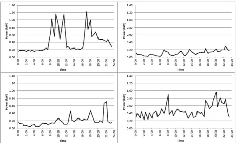
Although the demands were from domestic customers, there was a wide diversity in the
demands in terms of their time of day behaviour and their overall levels. For example,
Figure 3 shows the demands from the first four meters in the data set for a Friday in the
middle of the period. Apart from the values being lower in the early hours of the
morning and being relatively high around 18:00, there is little similarity between the
profiles. Figure 4 is the average demand from all the meters for this Friday and the
following Saturday. In contrast to the individual behaviour in Figure 3, the 96 meters
taken as a whole seem to have a distinct pattern of low night time, medium day time
and high evening demand. Figure 5 considers how the overall consumption over the
8,448 half hours differs for the customers. This histogram shows that if two customers
are chosen at random, then it is not uncommon for one to have two or more times the
consumption of the other.
In practice, the half hourly data will only be available from groups of meters. Figure 6
shows the average demands from meters 1 to 4, 5 to 8, 9 to 12 and 13 to 16 for the
Friday used in Figure 3.
3.2 Substation data
The smart meter data in Section 3.1 did not have any corresponding substation load
measurements available. Therefore, the meters were randomly assigned to phases and
the substation phase loads were based on the sums of the meters on each phase.
The background noise stemming from factors such as the cable losses was modelled as
4% of the total load supplied (in line with the low voltage losses estimated in [2]). This
was split in line with the ratio of the smart meter loads on each phase and added to the
substation phase loads. Finally, uncertainty in the allocation of this extra load to the
phases was modelled in Section 5.2.2 by altering the splitting ratio by 10%. For
example, for a 2 phase system, if the smart meter load split was 46:54 between red and
yellow, then the split of 56:44 was used for the allocation of the 4% cable losses term.
4 Readings available from individual smart meters
Access to the individual smart meter readings is sensitive as it can allow a profile of the customer’s behaviour to be constructed, especially if it is combined with other data sources such as social media accounts. For example, the top left demand profile in
Figure 3 suggests that the property might have been unoccupied between 12:00 and
unoccupied for the whole period. Consequently, the policy in the UK is that the data
from individual smart meters will only be available for network analysis for half hour time
periods if they are aggregated together with the values from other meters. However,
individual smart meter data averaged over longer periods such as a month are regarded
as being much less sensitive as it is more comparable with the energy usage readings of “old” meters. Hence the policy as stated in [3] is that “4.19 … network operators could access monthly consumption data from individual households for regulated
purposes”. However, this individual data is likely to be at a premium, and so it is
desirable to get as much information as possible from the grouped meter data to
augment the individual data.
5 Grouped smart meters
In contrast to the individual smart meter data, the number of time periods with grouped
smart meter data available to the UK’s DNOs will potentially be very large, e.g. there are
approximately 17,500 half hours in a year. The DNOs will be able to specify which
meters they want to be grouped together. A sensible way to group the meters is on the
basis of being close together and being believed to be on the same phase (as in Figure
1). However, as some of the believed phases may be wrong, some of the groups might
have a mix of phases (as in Figure 2). This section proposes and analyses an
approach for using the grouped data to identify the groups whose meters are believed
to be on a single phase but where there is actually a mix of phases. If the mixed and
single phase groups can be successfully identified, then this would allow the possibility
of analysing all possible phase combinations for the single meter data by just looking at
the possible phase permutations amongst the mixed groups. Hence the most
appropriate of the single meter phase identification techniques discussed in Section 2
could then be employed to determine the phasing breakdown in the mixed groups.
The approach’s steps are presented in Figure 7. In step 1, groups of meters are formed that are close to each other and which are believed to be on the same phase, e.g. from
the records from the time the customers were connected. The approach investigates whether a better fit between the substation data and the customers’ smart meter data can be achieved if some of the groups are designated as containing a mixture of phases
(with the mixture being specified, e.g. 3 red and 1 yellow). Therefore, step 2 modifies
the designation of the phases assigned to the groups to see whether this new
For each labelling combination, the groups of smart meters are used to predict the
current on each phase at the substation for each half hour (step 3), and this is then
compared with the recorded substation currents (step 4) to produce a prediction error.
How well each labelling of phases to groups does, is assessed by calculating the
variance of these errors (step 5). The labellings are then ranked on the size of these
variances, with the smaller the variance, the better the labelling (step 6). This ranking of
the different designations of phase labels to the groups of meters, can then be used to
either
select the best designations (step 7.a) that can then be analysed (step 7.b) using
the monthly individual smart meter data (see Section 4) along with one of the
approaches from Section 2, e.g. using the designation as the objective function for
the subset sum approach of Section 2.1,
or
identify the groups most likely to contain a mix of phases (step 8.a). Again the
approaches from Section 2 can then be used to identify the individual customer
phases for these groups using the monthly individual data (step 8.b) in a similar
way to step 7.b.
In more detail, step 3 estimates the substation load using the loads from the groups
allocated to this phase and a contribution from the loads from the mixed groups with at
least one meter on this phase. This mixed contribution is the value of the group load
times the fraction of this group on this phase times a (constant) scaling value. For
example, if a group is modelled as 3 meters on red and 1 on yellow, then its contribution
to the substation red phase total is 0.75the group totalthe scaling value.
In step 5, a single value for each allocation of groups to phases is produced by adding
together the variances from the different phases. When these values for all possible
group phasing permutations are ranked, the correct permutation is conjectured to have
one of the lowest values – the basis for this is detailed in Section 5.1.
The ranking value was analysed using the data sets of 96 smart meters with 8,448 time
periods introduced in Section 3. 96 was chosen as the number of meters for the
analysis as
It is close to 100 but is divisible by 3 and 4. This allowed group sizes of 2, 3 and 4 to be analysed on the same data set.
For ease of the implementation and of describing the approach, only two phases were
used in the modelling, i.e. red and yellow. The approach can easily be extended to
three phases but it becomes messier as it means there are more combinations for the
mixed groups, e.g. {2 red, 1 yellow, 1 blue}, {1 red, 3 yellow, 0 blue}, etc. The extension
to three phases is considered in Section 6. The 96 meters were allocated to groups in
terms of their numerical order, i.e. for a group size of 4, meters {1, 2, 3, 4} formed group
one, meters {5, 6, 7, 8} formed group two, etc. The meters were allocated to phases by
Assigning meters 1 to 48 to the red phase and meters 49 to 96 to the yellow phase (step 1). This corresponds to the prior beliefs, i.e. the recorded phases,
being that the first 48 meters were attached to the red phase and the second 48
meters were attached to the yellow phase.
Changing up to 4 of the 1 to 48 red meters to the yellow phase and up to 4 of the
49 to 96 yellow meters to the red phase, with the indices of the changed meters
being sufficiently well separated that they were in separate groups for groups of
sizes 2, 3 and 4 (step 2).
5.1 Variances of the correct and incorrect labellings
Considering the case of the prior beliefs about one of the first 48 meters and one of
meters 49 to 96 being incorrect, e.g. meter 48 is actually on the yellow phase and meter
96 is on the red phase, then if the groups containing meters 48 and 96 have been
correctly identified as being mixed, then the red component of the ranking measure for
group size 2 comes from the formula:
M47,t + M96,t– (M47,t + M48,t) – (M95,t + M96,t) Equation (1)
where Mi,t is the reading of meter i at time t.
Equation (1) stems from meters 1 to 46 being correctly identified as red, just leaving the
mixed groups containing meters 47, 48, 95 and 96 to affect the measure.
If we assume that the meter values are independently identically distributed and, without
losing any loss of generality, that the variance is 1, then the variance of equation 1 is
If the red mixed group is wrongly identified as meters 1 and 2 rather than meters 47 and
48, then the formula is now
M1,t + M2,t + M47,t + M96,t– (M1,t + M2,t) – (M47,t + M48,t) – (M95,t + M96,t)
The corresponding variance is
3 (1 –)2 + 1 + 2 = 4 2– 6 +4 Equation (3)
If in addition the yellow mixed group is wrongly identified as meters 49 and 50, then the
corresponding formula is
(1 –) (M1,t + M2,t) – M48,t + M96,t– (M49,t + M50,t)
and the corresponding variance is
2 (1 –)2 + 2 + 2 2 = 4 2– 4 +4 Equation (4)
Comparing equation (2) with equations (3) and (4), we can see that equation (4) is
always 2 greater than equation (2), and equation (3) minus equation (2) is 2 – 2 , and
so this is positive for less than one. Hence if is less than 1, then the variance of the
case where the mixed groups are correctly identified, i.e. equation (2), is less than the
cases where they are incorrectly identified, i.e. equations (3) and (4). In practice the
assumption that the meter values are independently identically distributed will not hold,
but the conjecture is that the ranking value corresponding to the correct labelling of the
mixed groups will be one of the lowest ranking values when the number of time periods
is large. Section 5.2 analyses this conjecture.
For group sizes of 3 and 4, the ranking formulae for the correctly identified mixed
groups are respectively
M46,t +M47,t +M96,t– 2 (M46,t +M47,t +M48,t) – (M94,t +M95,t +M96,t)
and
M45,t +M46,t +M47,t +M96,t– 3 (M45,t +M46,t +M47,t +M48,t) – (M93,t +M94,t +M95,t +M96,t)
The multipliers 2 and 3 stem from these mixed groups being designated as having 2
and 3 reds in them. and are used instead of so as to emphasise that the value of
the scaling factor depends on the group size. Expressions for the variances can be
derived in the same way as when the group size was 2. The intervals for and that
other variances, are smaller than the interval for group size 2 where the constraint was
<1, but they both contain the reciprocal of the group size.
5.2 Analysis of the ranking measure using the smart meter data
The approach of Figure 7 and Section 5.1 was applied to the data set of 96 smart
meters with values for 8,448 half hourly time periods (see Section 3.1). The substation
data was modelled as described in Section 3.2. Any discrepancy between the sum of
the meter readings for a half hour and the substation values, i.e. from the modelling of
the unmetered loads and losses, was split in the ratio of the totals from the believed
phasing of the meters, i.e. the 1 to 48 red total and the 49 to 96 yellow total. These
calculated discrepancies were then deleted from their respective substation phase
totals. Hence the sum of the grouped meter values equalled the sum of the substation
phase values.
The set of labelling schemes that were ranked (i.e. those considered in step 2) were
when all the mixed groups were correctly identified, when all but one of the mixed
groups were correctly identified, and when just one mixed group on each phase were
incorrectly identified, i.e. all but two of the mixed groups were correctly identified. For
example, for a group size of 4 and one incorrectly recorded meter for each phase, e.g.
meter 48 is on yellow and meter 96 is on red, then there is one correct labelling, 11
labellings with just the red mixed group wrong, 11 labellings with just the yellow mixed
group wrong, and 121 labellings with one red group and one yellow group wrong, giving
144 labellings in total (hence the 144 at the top of the second column in Table 1).
Therefore, all the labellings that are closest to the labelling initially believed to be correct
(step 1), have their ranking measure calculated (steps 2 to 6).
5.2.1 Zero unmetered loads
The adjustment to the unmetered load splitting ratio in Section 3.2 was set to zero
rather than 10%. One of the first 48 meters was assigned to yellow and one of the
second 48 meters was assigned to red, i.e. the number of mixed groups was 2. The
group size was set at 4. All 144 labellings for no mixed groups, 1 mixed group and 2
mixed groups were analysed. The labelling that corresponded to the correct
identification of the two mixed groups gave the lowest value, i.e. was ranked as 1 (in
step 7.a). This is denoted by the 1 in the first entry in column 3 row 2 of Table 1. This
meters 1 to 48 and the index of the red meter in meters 49 to 96. This gave the other
11 entries in the column 3 row 2 cell. These 12 ranking entries were converted to a
percentage ranking by dividing by 144 and multiplying by 100. The median, mean and
highest of these percentages are given in columns 4, 5 and 6. The analysis was
repeated with 4, 6 and 8 mixed groups to give rows 3, 4 and 5. Tables 2 and 3 give the
corresponding results when the group sizes were 2 and 3. Tables 1, 2 and 3 show that
the correct labelling is generally in the top fraction of a percent in the rankings when the
number of mixed groups is 4, 6 or 8.
In Table 4, the top 75 rankings from the bottom row of Table 1 are analysed, i.e. the
case of group size 4 and 8 mixed groups. For each of the 24 size 4 groups, the number
of times this group is labelled as a mixed group in these top 75 ranked labellings is
determined (step 8.a). For example, the group containing meters 1 to 4 might be
labelled as a mixed group in labellings with rankings of, say, 7, 32 and 66, giving an
overall score for this group of 3. Table 4 identifies whether the groups with scores of at
least 70, 60, 50 and 40 are actually mixed or not. The statistics in this table, e.g. the
mean, stem from analysing the 12 random assignments of meters considered in the
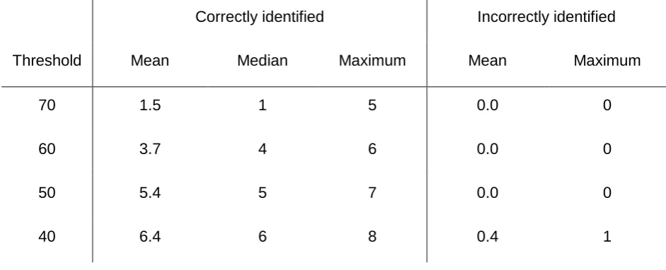
bottom row of Table 1. Table 4 shows that if the threshold is set at 80%, i.e. 60 out of
75, then approximately half of the 8 mixed groups can be identified with the chance of
an incorrect identification of a single phase group as mixed being extremely low.
However, the raw data (not presented here) showed that often the bottom one or two
mixed groups had counts well below many single phase groups.
Table 5 repeats the analysis of Table 4 but for groups of size 3 and 6 mixed groups, i.e.
the case of the bottom row of Table 2. As the choice of 75 for the number of rankings in
Table 4 was arbitrary, 50 rankings were used in Table 5 so as to investigate the effects
of a lower number. The results were similar to Table 4. Several of the mixed groups
could be very reliably identified when the threshold was set at 80% i.e. a count of 40 or
more, but some of the mixed groups had very low counts, and so were not identifiable.
Consequently, using the ranking measure with step 8.a seems to be able to very reliably
identify some but not all of the mixed groups. It is likely that this identification could be
improved by investigating what is the best number of rankings to use rather than the
5.2.2 Modelling the presence of unmetered loads
The 4% discrepancy between the substation loads and the sum of the smart meter
loads (see Section 3.2) was not split across the phases in line with the believed split of
smart meters across the phases, but the red percentage of this split was increased by
10% and the yellow percentage was decreased by 10%. For example, if the sum of the
smart meter loads believed to be on the red phase was 47% of the total of the smart
meter loads, then 57% of the discrepancy term was added to the substation’s red phase and 43% to the substation’s yellow phase.
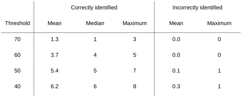
Table 6 gives the results from performing the same analyses as in Table 4. Comparing
Table 6 with Table 4 shows that the ranking approach performs similarly in both cases,
with Table 4 possibly performing slightly better when the threshold was 70.
In addition to cable losses, a proportion of the discrepancy between the substation and
the smart meter loads can arise from customer loads that are not metered. The effects
of some of these, e.g. street lights, could be ameliorated by considering the nature of
the load, e.g. it may only happen at night, but some of the loads will be more random.
Therefore, the ranking approach’s robustness to these loads was investigated by
allocating extra customer loads to the substation phases. Six extra profiles from the
same data set behind the 96 profiles in Section 3.1 were used, i.e. the analysis involved
102 different profiles. The test involved adding extra customer loads to the case
analysed in Table 6, i.e. the case of a 10% imbalance in the cable losses being added
to the red phase. Most of the majority of these extra customers were added to the red
phase so as to worsen the effect of the cable loss imbalance. The cases considered
were 2 meters on red and 1 on yellow, 4 meters on red and 2 on yellow, 4 metres on
red and 1 on yellow, 5 metres on red and none on yellow, and 6 metres on red and
none on yellow. For each of these, the 12 cases considered in each row of Table 6
were analysed. The results are given in Table 7. The deterioration in the performance
as the number of extra unmetered loads on the red phase compared with the yellow
phase increases from one to six is very low.
Tables 6 and 7 show that the performance of the ranking approach in reliably identifying
some of the mixed groups is robust to the presence of unmetered loads with no meters
being wrongly identified in 10 out of the 12 cases making up each row, and only 1
6 Discussion
Several simplifications were made in the modelling:
2 phases – The analyses in Section 5 were carried out on two phases rather than three. For the three phase case it seems simpler and more straightforward to perform three “2 phase” analyses, i.e. red, and non-red, etc., than to perform one combined analysis.
Meter inaccuracy – The high degree of accuracy required from the meters for
billing purposes means that this is unlikely to lead to serious mismatches
between the substation and the smart meter totals in practice. Meter inaccuracy
was modelled in [11] with no problems being found. Where concerns have been
raised over the accuracy of smart meters, it has been when the waveforms are
distorted rather than for more normal conditions (see for example [16]).
The number of meters aggregated together – This research has considered group sizes of 2, 3 and 4. As the group size increases, phase identification
becomes more difficult. However, group sizes much above 4 are probably not
that helpful for network analysis anyway as the meters being aggregated
together become more spread out through the network.
7 Conclusions
The proposed method for analysing grouped smart meter data can reliably detect some
of the mixed phase groups when the existing knowledge about the phase connections is
good but not perfect. The identification of the mixed groups is robust to the presence of
unmetered loads such as cable losses and unmetered customers.
This capability is important as the access to non-grouped smart meter data in the UK
will be very severely restricted, and so extracting information from the grouped smart
meter data will be paramount.
Notation
Mit is the ithsmart meter’s value at time t
Rt is the red phase value at the substation at time t
Xi is 1 if the ith smart meter is connected to the red phase and 0 otherwise
is the scaling value applied to mixed groups of size 2 (see Section 5)
is the scaling value applied to mixed groups of size 4 (see Section 5
Acknowledgements
We would like to thank the CLNR project team for providing us with the Smart Meter
datasets necessary to carry out this research, and the insightful comments of the
anonymous referees.
References
[1] EurElectric (2013) Power distribution in Europe facts and figures
http://www.eurelectric.org/media/113155/dso_report-web_final-2013-030-0764-01-e.pdf (Accessed 13th December 2017)
[2] Sohn Associates (2009). Electricity distribution system losses: Non-technical
overview
https://www.ofgem.gov.uk/ofgem-publications/43519/sohn-overview-losses-final-internet-version.pdf (Accessed 13th December 2017)
[3] DECC (2012) Smart metering implementation programme: Data access and privacy – Government response to consultation Department of Energy and Climate Change https://www.gov.uk/government/uploads/system/uploads/attachment_data/file/43046/7
225-gov-resp-sm-data-access-privacy.pdf (Accessed 13th December 2017)
[4] Strbac, G, Djapic, P, Ortega, E, Stanojevic, V, Heyes, A, Markides, C, Aunedi, M,
Shamonina, E, Brook, R, Hawkins, D, Samuel, B, Smith, T, & Sutton, A (2014)
Management of electricity distribution network losses Imperial College / Sohn
Associates
https://www.westernpower.co.uk/docs/Innovation-and-Low-Carbon/Losses-strategy/SOHN-Losses-Report.aspx (Accessed 13th December 2017)
[5] Pezeshki, H, & Wolfs, PJ (2012) Consumer phase identification in a three phase
unbalanced lv distribution network Proceedings of the 3rd IEEE PES Conference on
Innovative Smart Grid Technologies (Available on IEEE Xplore)
DOI:10.1109/ISGTEurope.2012.6465632
[6] Arya, V, & Mitra, R (2013) Voltage-based clustering to identify connectivity
relationships in distribution networks Proceedings of 4th IEEE International Conference
on Smart Grid Communications (Available on IEEE Xplore)
DOI:10.1109/SmartGridComm.2013.6687925
[7] Fan, Z, Chen, Q, Kalogridis, G, Tan, S, & Kaleshi, D (2012) The power of data: Data
Innovative Smart Grid Technologies (Available on IEEE Xplore)
DOI:10.1109/ISGTEurope.2012.6465630
[8] Arya, V, Mitra, R, Mueller, R, Storey, H, Labut, G, Esser, J, & Sullivan, B (2014)
Voltage analytics to infer customer phase Proceedings of the 5th IEEE PES
Conference on Innovative Smart Grid Technologies (Available on IEEE Xplore)
DOI:10.1109/ISGTEurope.2014.7028878
[9] Seal, BK, & McGranaghan, MF (2011) Automatic identification of service phase for
electric utility customers Proceedings of the IEEE Power and Engineering Society
General Meeting (Available on IEEE Xplore) DOI:10.1109/PES.2011.6039623
[10] Short, TA (2013) Advanced metering for phase identification, transformer
identification, and secondary modelling IEEE Transactions on Smart Grid 4(2)
651-658 DOI:10.1109/TSG.2012.2219081
[11] Arya, V, Seetharam, D, Kalyanaraman, K, Dontas, K, Pavlovski, C, Hoy, S, &
Kalagnanam, JR (2011) Phase identification in smart grids Proceedings of 2nd IEEE
International Conference on Smart Grid Communications (available on IEEE Xplore)
DOI:10.1109/SmartGridComm.2011.6102329
[12] Mangasarian, OL & Recht, B (2011) Probability of a unique integer solution to a
system of linear equations European Journal of Operational Research 214(1) 27-30
DOI:10.1016/j.ejor.2011.04.010
[13] Duran, A (2015) Smart Meter Aggregation Assessment EA Technology report
http://www.energynetworks.org/assets/files/electricity/futures/smart_meters/FINAL%20
REPORTS%20from%20consultants/Smart%20Meter%20Aggregation%20Assessment
%20Final%20Report%20-%20Executive%20Summary_V1%204%20FINAL.pdf
(Accessed 13th December 2017)
[14] Lees, M (2014) Enhanced network monitoring Customer-Led Network Revolution
CLNR-L232 http://www.networkrevolution.co.uk/resources/project-library/ (Accessed
13th December 2017)
[15] Bulkeley, B, Matthews, P, Whitaker, G, Bell, S, Wardle, R, Lyon, S, & Powells, G
(2015) Domestic Smart Meter Customers on Time of Use Tariffs Customer-Led
Network Revolution CLNR-L243
[16] Leferink, F, Keyer, C, & Melentjev, A (2016) Static energy meter errors caused by
conducted electromagnetic inference IEEE Electromagnetic Compatibility Magazine
Table 1: The ranking of the correct designation of which groups are mixed out of all the permutations of assigning the correct number or less of mixed groups to the 24 groups when the group size was 4 (i.e. the results of step 7.a).
Number of
mixed
groups
Number of
phasing
labellings
Ranking of the correct designation for 12 different
allocations of meters to phases different from their
believed phase
Median % Mean % Worst %
2 144 1, 28, 4, 1, 7, 1, 1, 1, 1, 1, 1, 7 0.69% 3.13% 19.44%
4 4,356 1, 3, 2, 1, 161, 6, 1, 1, 1, 1, 6, 4 0.03% 0.36% 3.70%
6 48,400 427, 128, 7, 7, 274, 175, 1, 53, 8, 71, 44, 30 0.10% 0.21% 0.88%
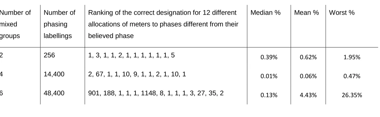
Table 2: The ranking of the correct designation of which groups are mixed out of all the permutations of assigning the correct number or less of mixed groups to the 32 groups when the group size was 3 (i.e. the results of step 7.a).
Number of
mixed
groups
Number of
phasing
labellings
Ranking of the correct designation for 12 different
allocations of meters to phases different from their
believed phase
Median % Mean % Worst %
2 256 1, 3, 1, 1, 2, 1, 1, 1, 1, 1, 1, 5 0.39% 0.62% 1.95%
4 14,400 2, 67, 1, 1, 10, 9, 1, 1, 2, 1, 10, 1 0.01% 0.06% 0.47%
6 48,400 901, 188, 1, 1, 1, 1148, 8, 1, 1, 1, 3, 27, 35, 2 0.13% 4.43% 26.35%
Table 3: The ranking of the correct designation of which groups are mixed out of all the permutations of assigning the correct number or less of mixed groups to the 48 groups when the group size was 2 (i.e. the results of step 7.a).
Number of
mixed
groups
Number of
phasing
labellings
Ranking of the correct designation for 12 different
allocations of meters to phases different from their
believed phase
Median % Mean % Worst %
2 576 1, 1, 1, 1, 10, 1, 1, 1, 1, 1, 1, 2 0.17% 0.32% 1.74%
Table 4: The split between whether the most commonly occurring mixed groups in the top 75 rankings were actually mixed or not when the group size was 4 and the number of mixed groups was 8 (i.e. the results of step 8.a).
Correctly identified Incorrectly identified
Threshold Mean Median Maximum Mean Maximum
70 1.5 1 5 0.0 0
60 3.7 4 6 0.0 0
50 5.4 5 7 0.0 0
40 6.4 6 8 0.4 1
Table 5: The split between whether the most commonly occurring mixed groups in the top 50 rankings were actually mixed or not when the group size was 3 and the number of mixed groups was 6 (i.e. the results of step 8.a).
Correctly identified Incorrectly identified
Threshold Mean Median Maximum Mean Maximum
50 1.8 2 3 0.0 0
45 2.4 2 3 0.0 0
40 3.0 3 4 0.0 0
35 3.4 3 5 0.1 1
Table 6: Repeating the analysis of Table 4 but using 10% rather than 0% to adjust the split of the cable loss discrepancy between the substation load and the sum of the smart meter loads (i.e. the results of step 8.a).
Correctly identified Incorrectly identified
Threshold Mean Median Maximum Mean Maximum
70 1.3 1 3 0.0 0
60 3.7 4 5 0.0 0
50 5.4 5 7 0.1 1
40 6.2 6 8 0.3 1
Table 7: Identifying the mixed phase groups after adding unmeasured meters to the substation for the 10% imbalanced losses case of Table 6. The threshold for identifying the mixed groups was 80% (i.e. the results of step 8.a).
Unmetered Correctly identified Incorrectly identified
red and
yellow
Mean Median Maximum Mean Maximum
0 and 0 3.7 4 5 0.0 0
2 and 1 4.0 4 5 0.2 1
4 and 2 4.2 4 6 0.2 1
4 and 1 4.3 4 6 0.2 1
5 and 0 3.6 4 5 0.2 1
Figure 1: Believed phasing according to the network records. Smart meters are allocated to groups based on proximity and their believed phase.
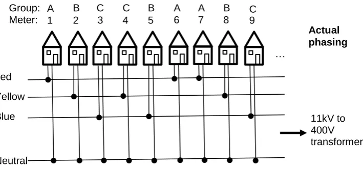
Figure 2: Actual phasing. Meters 4 and 5 are on different phases to those they are believed to be on in Figure 1, and so groups B and C now contain a mixture of meters connected to the yellow and blue phases.
Neutral Blue Yellow Red
11kV to 400V transformer
Meter: 1
Group: A
Believed phasing
2 3 4
B C C
5 6 7 8 9
B A A B C
…
Neutral Blue Yellow Red
11kV to 400V transformer
Meter: 1
Group: A
Actual phasing
2 3 4
B C C
5 6 7 8 9
B A A B C
[image:24.595.88.443.335.501.2]Figure 3: The first four profiles in the smart meter data set for Friday the 7th of February
Figure 4: The average demand from the 96 meters for each half hour on Friday the 7th
and Saturday the 8th of February 2014.
[image:26.595.75.349.487.656.2]Figure 7: The steps in using grouped smart meter data to improve the identification of customer phases
1) Original designation of groups as being on the red, yellow or blue phases
2) Alter original designation by
specifying some groups as mixed phase
3) Predict the half hourly totals for the red, yellow and blue phases at the substation
5) Calculate the variance of the half hourly errors
8.a) Find groups labelled as mixed in the lowest variance designations 7.a) Find the
designations with the lowest variances Smart meter group totals Substation phase totals Individual smart meter monthly totals
4) Form the half hourly errors between the prediction and the observation
7.b) Check all the individual customer phasings for each mixed group
Start
6) Sort the phase designations in order using the size of their variances Test phase designations
For each half hour
Phase recorded at time of connection