Actuarial models for the analysis of disability income insurance

(1)

ACTUARIAL MODELS FOR THE ANALYSIS OF DISABILITY

INCOME INSURANCE

By

David G.W. Pitt

November 2004

(2)

To my parents,

(3)

DECLARATION

This thesis contains no material which has been accepted for the award of any other degree or diploma in any other university, and to the best of my knowledge and belief, this thesis contains no material published or written by another person, except where due reference is made in the thesis.

(4)

ABSTRACT

(5)

ACKNOWLEDGEMENTS

(6)

LIST OF FIGURES

Figure 2.1 Multi-state model used for Disability Income Insurance Modelling... 7

Figure 2.2 General Insurance Claim History Model... 14

Figure 3.1: Comparison of Actual and Expected Experience over Tim e... 29

Figure 3.2: Reserve requirements to obtain varying probabilities of adequacy...41

Figure 4.1: Kaplan-Meier Estimate of the Claim Duration Survival Function...56

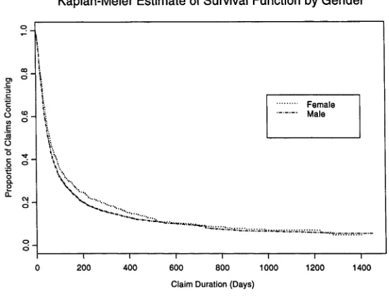
Figure 4.2 Kaplan-Meier Survival Function Split by Gender... 57

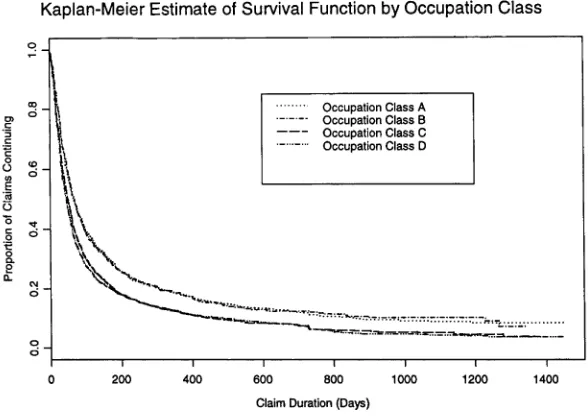
Figure 4.3 Kaplan-Meier Survival Function Split by Occupation C lass... 58

Figure 4.4: Kaplan-Meier Survival Function Split by Deferment Period... 58

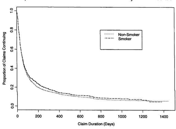
Figure 4.5: Kaplan-Meier Survival Function Split by Smoker Status... 59

Figure 4.6: Cumulative Hazard Ratio Plots for Various Levels of Independent Variables... 63

Figure 4.7: Assessment of Fit of Parametric Density to Claim Duration... 68

Figure 4.8: Comparison of Actual and Fitted Rates for the Generalised F Distribution... 77

Figure 4.9: Comparison of Kaplan-Meier and Cox Regression Claim Duration Models... 78

(11)

Figure 5.2: Comparison of Sensitivities of Log Duration to Age...91

Figure 5.3: Comparison of Sensitivities of Log Duration to Occupation C lass... 91

Figure 5.4: Density Function of Mean Difference CRQ vs Cox Regression Survival (0.8,1.0)...94

Figure 5.5: Density Function for Mean Difference CRQ vs Cox Regression Survival (0.6,0.8)... 95

Figure 6.1: Multiple State DII M odel... 97

Figure 6.2: Supersmoothed Hazard Rates for Claim Termination...99

Figure 6.3: Three step tree diagram for Calculation of Premium Rates... 104

Figure 6.4: Risk Premia by Occupation Class... 109

Figure 6.5: Risk Premia by Benefit Level... 110

Figure 6.6: Risk Premia by Deferred Period... 110

Figure 6.7: Flowgraph for Disability Income Insurance Contract... 112

Figure 6.8: Revised Flowgraph with Single Output State... 113

(12)

LIST OF TABLES

Table 3.1: Table of Covariates for GLM Analysis...25

Table 3.2: Summarised Rating Variables...26

Table 3.3: Comparison of Actual and Expected Experience over Time... 30

Table 3.4: Index of Termination Rates by Characteristic...31

Table 3.5: Retained Covariates... 38

Table 3.6: Reserve requirements for probability of adequacy... 42

Table 3.7: Incidence Rate GLM Coefficients...44

Table 3.8: IAD vs GLM incidence rates for two-week deferred period...47

Table 3.9: IAD vs GLM incidence rates for one-month deferred period...48

Table 3.10: Goodness of Fit Analysis... 50

Table 4.1: Potential Covariates for Claim Termination Rate Analysis...53

Table 4.2: Summary of Potential Claim Duration Parametric Distributions... 66

Table 4.3: Assessment of Fit of Parametric Density to Claim Duration...69

Table 4.4: Assessment of Accelerated Failure and Mixture Models for Claim Duration...73

(13)

Table 4.6: Logistic Model Regression Coefficients 76

Table 4.7: Annuity Value Comparison for three Model Fitting Procedures... 79

Table 5.1: Censored Regression Quantile Coefficients... 87

Table 5.2: Censored Regression Quantile Output... 88

Table 6.1: Estimated Regression Coefficients - Claim Termination Rate Analysis...100

Table 6.2: Duration Bands for Recovery Intensities... 106

Table 6.3: Groups of Lives for risk premium calculations... 109

Table 6.4: Piecewise Exponential Model for Claim Recovery Intensities...118

(14)

CHAPTER ONE

INTRODUCTION

1.1 Introduction and Motivation

Between 1988 and 2001, the in-force annual premiums for Australian disability income insurance (DII) have increased from 180 million dollars to almost 1.1 billion dollars (Munich Re of Australia, Rice Kachor Research (2002)). This increase has occurred across both ordinary and superannuation linked lines of life insurance risk business. This sharp increase in the volume of DII business, and the inherent difficulty in calculating actuarially fair premium rates for this line of business, provided the motivation for the research presented in this thesis.

(15)

Expenses play a particularly important role in the determination of premium rates for DII business. DII business is predominantly sold through insurance brokers and agents, and hence large initial expenses related to commissions are common. Once a DII contract has been signed, the renewal expenses (payable generally annually) are significantly lower than the expenses that the office faces in the first year after initial sale. It is therefore of interest for insurers to have a measure of the persistency, or renewal rates, for those insured lives who have purchased DII in the past. Higher renewal rates will lead to lower expenses on average each year and in turn can justify lower premium rates.

The largest and most uncertain future cash outflow in the management of DII business arises due to the payment of the insured disability benefits. Uncertainty in the amount of these cash flows stems from two sources: first, the occurrence of future disability for an insured life is uncertain; and second, the duration of a claim under a DII contract can vary from as little as one week to many years. It is common actuarial practice (Booth, 2000) to estimate the rate of disability onset using a claim incidence rate and to estimate the duration of claims using a set of estimated claim termination rates.

A number of morbidity tables have been produced, based on the disability experience of life offices, in various countries. These tables provide practising actuaries with a starting point for the assessment of their future liabilities associated with in force DII business. These tables include (Munich Re, 2002):

• The Manchester Unity Tables (covering a lengthy nineteenth century investigation in England);

(16)

The Commissioner’s Individual Disability Tables (CIDA) 1985; and

• The Australian Table IAD89-93.

The construction of the Australian Table and also some of the experience analysis performed in the UK will be reviewed in Chapter 2 of this thesis.

1.2 Contribution of this Thesis

This thesis proposes the use of a number of recently developed statistical methodologies to the actuarial pricing of DII business. Experience analysis of DII business overseas and in particular in Australia has up until now relied on statistical methods developed over thirty years ago. Multiple state modelling, exposed-to-risk and graduation methods along with actual vs expected analysis have formed the historical basis for the modelling of claim incidence and claim termination rates. These forms of modelling do not readily capture interactions that exist between the rating variable information available to DII providers. Historically popular methods rely on subdividing DII data prior to performing analysis to enable faster computation of output. Faster computing speeds and increased statistical literature that makes use of these methods, enables considerably more data analysis to be performed on DII policy and claim data.

(17)

termination. The results of this modelling will then be used with existing actuarial pricing theories to develop suitable premium rates and reserving strategies for DII business.

1.3 Structure of Thesis

Chapter Two will provide a review of the most important literature relating to the analysis of DII business from an actuarial and statistical viewpoint. This will place the research that follows in an appropriate context.

Chapter Three will report the results of two generalised linear model analyses of DII claim experience presented to the Institute of Actuaries of Australia membership in 2002 and 2003. The termination rate analysis in that chapter was published in the Australian Actuarial Journal and the incidence rate analysis formed part of the Proceedings of the 2003 Biennial Convention of the Institute of Actuaries of Australia.

Chapter Four continues the analysis of claim termination rates with the use of survival models for long term survivors (Mailer and Zhou, 1996). Survival analysis provides a natural modelling framework for the analysis of disability claim durations. Both claim termination rates and probabilities of failure to recover are modelled in terms of various sets of underlying covariates or rating factors.

(18)

example, assess whether the impact of smoker status on claim termination varies according to the duration that a claimant has already been receiving DII benefits. This is an important feature of the analysis because the calculation of disabled life reserves depends critically on the impact of covariates at a range of claim durations.

Chapter Six ties together some of the work presented in earlier chapters and develops actuarial pricing strategies using both multiple state models and flowgraph models.

Chapter Seven concludes the thesis. A summary of the main findings of the research is given along with recommendations for future research.

Acknowledgement

(19)

CHAPTER TWO

LITERATURE REVIEW

2.1 Disability Income Insurance Models

The development of a number of different models for the description of disability income insurance (DII) has taken place over the last two decades. The models proposed have varied considerably in terms of underlying assumptions, the amount of underlying statistical rigour and the extent of data used in their development. This section will review a number of the key papers on DII, and place the research work developed in this thesis in context.

2.1.1 Continuous Mortality Investigation Reports

(20)

as a key method for the pricing and reserving in respect of DII policyholders. The multiple state model used in the analysis is shown in Figure 2.1 below.

DEAD ABLE

Insured is able to work and earn income

ILL

Insured is unable to work - either full or partial

disability.

Figure 2.1: Multi-state model used for Disability Income Insurance Modelling. A policyholder may move between the 3 states, with death an absorbing state

CMIR 12 begins by explaining the link between transition intensities and conditional probabilities for the state occupied by policyholders. Discussion then turns to the graduation of claim recovery and mortality intensities. In order to simplify the analysis and without loss of generality, Male Standard lives are the only lives considered in the report. After considerable experimentation, the complete formula used for the graduation of recovery rates derived in CMIR 12 was

p Ttsz=r.{a + b(\ + q . m a x ( 4 - w z , 0 ) ) . J Z ( Y - 5 0 ) } e - ‘'ß (2.1)

where a, b, c, p, q and s are constants and

p y+Z i is the transition intensity (or hazard rate) for recovery of a life aged y + z who has been

in the disabled state for a continuous period of z years

(21)

for z<5, Y = y

T = y + z - 5 fo rz> 5 ;

z is duration of sickness (in years) and

Z = z for z < 1,

Z = \ + s ( z ~ \ ) f o r l < z < 5 ,

Z = 1 + 4s for z>5

( i A

and for deferred periods of 4, 13 and 26 weeks, we have r = min^/? + — (wz - d ) ( \ - p ) , \

so that r — 1 if wz > d + 4 for deferred period d, expressed in weeks. Note also that w is a constant equal to the number of weeks in a year, taken as 52.18 in this analysis.

Equation (2.1) represents a stochastic model for the transition intensity from the disabled state to the able state. The model is fit using slices of data from the CMIR12 investigation where the slices contain recovery data for lives with specified age, deferred period and duration of disability characteristics. The above formulation was determined after various diagnostic checks on relationships present in the data. In particular, a plot of the log of the duration of claim effect (on claim termination rates) against the square root of duration produced a graph that was

(22)

underlying DII policy. This phenomenon suggests the need to model an interaction between age and deferred period in the description of claim termination rates - this interaction is explored more fully in Chapter 3, which focuses on generalised linear models and claim termination and

incidence rates. This interaction is dealt with in equation (2.1) by the term Vz (T -5 0 ) included

in the slope coefficient. There is also evidence of lower recovery rates during the periods soon after claim payments commence. These are dealt with in equation (2.1) by the reduction factor, r, which only applies for the period 4 weeks after the expiry of the deferred period. Evidence of an increased sensitivity of claim termination rates to age during the first four weeks of disability

is dealt with by the g.max ( 4 - wz,0) term in equation (2.1).

The graduation formula (2.1) was fitted using the method of maximum likelihood. A general discussion of maximum likelihood in the context of actuarial experience analysis is given in Forfar et al (1988). An experience analysis is the term used by actuaries to describe the investigation of a set of statistical data that is derived from business transactions over a long period. The most common experience analysis performed by actuaries is an investigation into mortality rates using data on deaths derived from payments of sums insured under endowment and term life insurance business. The use of maximum likelihood estimation means implies asymptotic standard errors for the estimated parameters in (2.1) are readily available. In addition, Bayliss (1991) tested the suitability of these standard errors by a method of simulating the experience and parameter-fitting process. His results were very close to those found using the asymptotic results based on maximum likelihood theory.

(23)

find evidence of a “hump-backed curve” relating the mortality experience to duration of disability. That is, mortality rates appear to be higher at shorter durations of disability claim (less than 20 weeks), regardless of the age of the claimant. The impact of increasing age on mortality rates is really only evident for ages greater than 50, where there is some evidence of the usual positive relationship between age and mortality rates.

The graduation of sickness inception intensities is also considered in CMIR12 (1991) by Waters. The method used is to separate data on exposure to the risk of claim inception and number of claims by age and deferred period. Separate graduations are performed for each of the four main deferred periods, namely 1 week, 4 weeks, 13 weeks and 26 weeks. Again experimentation with a range of functional models led to the use of

ax

= exP {/(■*)}> (2.2)

where

a x

represents the transition intensity (or hazard rate) for the transition from the able state

to the disabled state, x represents age and/ is usually a polynomial of degree three. This form of mathematical function and underlying model used for claim inceptions suggested the use of generalised linear modelling as a natural modelling approach. Higher sickness inception intensities were predicted for shorter deferred periods. In addition the impact of age was to increase the claim rates for both the youngest and oldest ages of the insured lives. That is, the sickness inception intensities were highest for those insured lives younger than 30 or older than 55. The impact of age on sickness inception intensities was greatest for the one week deferred period. The sickness inception intensities for the 26-week deferred period policies showed little evidence of a relationship with age - the graduated sickness inception intensities were about

(24)

CMIR12 (1991) next provides details on the computational procedures for determining both probabilities of movement between, or occupancy of, various states in the three state model in Figure 2.1. In addition the approximation of monetary functions using numerical integration methods was also described. Chapter Six of this thesis considers numerical methods for dealing with the semi-Markov nature of the transitions from the disabled state and the associated calculations of premium rates and disabled life reserves. Chapter Six will also demonstrate a new use of flowgraphs to calculate DII premium rates.

2.1.2 Significant Contributions to the Disability Income Insurance Modelling Literature

Many other models have been proposed in the literature for the pricing and reserving of disability income insurance. Gregorius (1993) describes the methodology used in the Netherlands. The potential annuity of benefits payable up until retirement under a DII contract is broken into two separate parts, the A-cover and the B-cover. The A-cover includes all payments to insureds for the first year of disability. A simple multiplicative model is used to calculate the risk premium in respect of the A-cover. The risk premium is calculated as

P ( i J , k ) = B.a(i). b(j). c(k), (2.3)

(25)

mortality rates for active and disabled lives, however, there is inadequate data in the Netherlands DII market to assess this theory. In order to deal with the duration dependent recovery rates, Gregorius proposes a refinement of the usual three state model used in DII analysis. The disabled state is divided into six states where each state denotes disability for a different amount of time. To simplify the calculations, a model without return, where transitions out of the disabled state are ignored is proposed for the determination of single premiums. This simplification clearly introduces significant bias into the analysis proposed by Gregorius.

Taylor (1971) introduced a Markov model with multiple states for duration of disability. This paper was key to the development of stochastic analysis in morbidity studies. This work was developed further by Haberman (1984).

Segerer (1993) describes the actuarial treatment of the disability risk in Germany, Austria and Switzerland. In these countries, and a number of other European centres, the method of pricing and reserving for DII is based on multiple decrement tables (Neill, 1977). The decrements are state dependent. For active lives, the two decrements of primary interest are mortality and disability. For those lives in the active state, the two decrements are recovery and mortality. The formula used in Switzerland for a net single premium is

__

1

_

N - N .

• — i

x+t+l/2 ’f x + f ' S x+t '^ x + t+ V 2 :n -t-l/2 \ ’ (2.4)

where Nx and Dx are standard actuarial commutation functions evaluated using national

mortality rates and 3% per annum interest, ix is the incidence rate of disability at age x, gx is factor that reflects the degree of the disability and a 1-^ represents the expected present value of

(26)

continuing for a maximum period of n years. Interestingly, the disabled life reserves are calculated based on standard life annuity values, reduced by a factor to allow for the fact that payment is made contingent on both survival and continuing disability. The formula used for the calculation of disabled life reserves is

V '= 1.02 a —,

1 x x+t:n-t\

W 5

/w+i

(2.5)

where

/ x (jc-1 5 )2 f i x ) = 0.3 +

0.7---v ' 50

Hert,f(x) is the age-dependent deduction factor and tV ‘ represents the amount of money that an insurer should hold in reserve in respect of a DII policy that was bought t years ago by a life that has just become disabled and was aged jc at the outset of the policy. At age 15, the factor is 0.3 and the factor increases continuously until it reaches unity at age 65. An age-dependent deduction factor of one implies equality between the standard life table annuity value and the disability annuity. The approaches adopted in Germany and Austria are slight variations on the approach in Switzerland. See Segerer (1993) for details. The underlying disability incidence and continuance rates used in Equations (2.4) and (2.5) are based on industry average statistics split by age and duration. Following tariff reform in parts of Europe in the early 1990s that impacted premium calculations, large loadings of up to 50% were added to previously used rates to bring them closer into line with industry experience.

(27)

0~IBNR 3~Settled -Reported

No Case Reserve

2~Reported Case Reserve

Figure 2.2 General Insurance Claim History Model

(28)

amount of the various payments made on transition between the states of the model in Figure 2.2. These data can be used to derive both probability distributions for payments made on transitions between states and the transition intensities for movement between states. The expected future payments on a claim that occurred at time u in the IBNR state is

where ymn (£) is the average payment made on transition from state m to state n, p0m («,£) is the

probability of a transition from state 0 to state m in the time between u and g and Amn (£)

denotes the transition intensity between states m and n at time £. Under the assumption of a Poisson process for claim arrivals and settlements, the transition intensities are constant and therefore the calculation of the transition probabilities between states can proceed by solving the usual Kolmogorov’s equations, (see for example, Pitacco et al (1999)).

Originally, actuarial pricing and reserving theory was developed on the basis of the calculation of expected present values of cash flows. The argument put forward for relying solely on deterministic calculations was that this approach was justified for large portfolios of insurance business due to significant pooling. More recently, this approach has been justified, in some cases, by the use of stochastic models. Norberg (1996) develops ordinary differential equations for moments of present values of benefits commonly found in life insurance. Norberg (1991, 1992) defines a set of notation in relation to a multistate life insurance policy. The policyholder can reside in any of J states at time t. These J states may include healthy, sick, lapsed, totally and permanently disabled (TPD) and dead. Let / / be an indicator variable for whether the

(29)

state k during the time interval (0, t]. The payment function B generated by the policy is assumed to be of the form

d B = Y j I!d B ;+ Y Jbild N !\ (2.7)

j j*k

where each B ’ is a deterministic payment function specifying payments due during sojourns in state j and each bjk is a deterministic function specifying payments due upon transition from state j to state k.

The present value of future benefits less premiums, that is the actuarial reserve, at time t is

- f (2.8)

v, ,

where v, is the standard discount factor. Norberg presents a theorem for finding the gth conditional moment of the present value in (2.8), given the information available at time t, that is

V qU) = E

( i n

Y

— f

vdB

U r

J

1

= i ,

J

(2.9)

where V q(J) represents the qth quantile of the distribution of the present value of future

payments under a DII contract, that is a contract that continues to make payments to this life while he resides in the disabled state, state j.

(30)

(b/k)rV,{q-r)k. (2.10)

d_

dt

=

(qS/ +ß! ) v ^ i -qb:v^-')l

k * j r- 0 V ^ >

This thesis will further explore moments of present values of projected benefits less premiums in the case where the assumptions of the Norberg model do not apply - in particular in relation to disability income insurance where Markov transition intensities are invalid. Instead, semi- Markov transitions from the ill state to the able state and the associated complications for premium rating and reserving will be considered in this research.

2.1.3 Australian Industry Table

During 1995, the Graduation Sub-Committee of the Disability Committee of the Institute of Actuaries of Australia produced an industry table of claim incidence and claim termination rates based on the experience of Australian disability income insurance policyholders in the years between 1989 and 1993 inclusive. The table is now presented as an Excel spreadsheet model and

is used to varying degrees by many of the large Australian life insurers which sell DII.

(31)

The data was graduated by fitting formulae so that the chi-squared measure of goodness of fit (Benjamin and Pollard (1993)) was minimised. The formulae used for the graduation were chosen after considering the shapes apparent in the CIDA (US experience based) tables. Given that many Australian insurers, at the time of preparation of IAD89-93, used the CIDA tables as a base and then made appropriate adjustments to fit their own experience, it was decided to form the IAD89-93 table without making any reference to the CIDA tables. This approach would mean that the Australian derived table would not contain any systematic bias due to country- specific conditions and could be used by insurers independently of other internationally derived morbidity tables.

In the construction of IAD89-93, separate curves were fitted, varying with age, for male accident incidence rates and male sickness incidence rates. The formula used for accident incidence rates was a cubic function of age:

F (x) = A + Bx + Cx2 + Dx3, (2.11)

where x represents the age last birthday at date of disablement. The accident incidence rate data is calculated using the number of accident induced new DII claims divided by the number of years that lives are observed in the able state, with a DII policy, and therefore are exposed to the risk of accident. Similarly for male sickness incidence rates, the formula adopted was

F( x) = A + Bx + CDx. (2.12)

(32)

B, C and D and for each of the 2 week and 1 month deferment periods. Other rating factors such as smoking status and other more unusual deferment periods had insufficient data, (for example six month deferred periods,) to warrant graduation. The report on the construction of the IAD table does provide some guidance to users on how to adjust the published rates for each of these factors, though this advice is more indicative than comprehensive.

For the determination of female incidence rates for both sickness and accident, sufficient data again was not available to warrant a reliable graduation of these rates. Instead a decision was made to adjust the male rates by a factor which varies according to age, deferment period, cause of claim (accident or sickness) and occupation class. After considerable experimentation, the formula chosen was

where/denotes female incidence rates, m denotes male incidence rates, c is the claim cause, X is age last birthday at disablement, o represents the occupational class and w represents the waiting period (either 2 weeks or 1 month). The quantities Ec X o w are the fitted factors varying by cause,

age, occupation class and deferment period. The Ec X o w factor is an adjustment factor that

applies to predetermined accident incidence rates and was modelled using

where Faow is a cubic polynomial as defined in (2.11) and for ages below M ow the formula

used was

(2.13)

(33)

female rate = male rate at age M o w.Fao w [ \ - G a w( X - M o w)\. (2.15)

The rationale behind the use of Equation (2.15) for low ages was to account appropriately for the “accident bump” present in the male incidence rate curve and to allow a straight line to be fitted for ages below Mow. Similar adjustments were made to the male sickness incidence rates to

estimate the female sickness incidence rates.

The monthly equivalent termination rates for each of the 2 week and 1 month deferment period claims were graduated using the formula

YXd = Ad {\ + B(l.X)-,d = 1 to 6 or 7, (2.16)

where YXij is the modelled value for the number of claims closing for lives aged x with claim duration d divided by the number of months that lives are aged x and disabled with duration d

months and X is the age last birthday. The values of d from 1 to 6 or 7 correspond to the durations as presented in the 1995 Disability Committee Report of the Institute of Actuaries of Australia. These are the periods ending at 1,3, 6, 12, 18, 24 and 36 months from disablement, with the 1 month duration only being relevant for the 14 day deferment period. Note that Aj

(34)

Monthly equivalent rates are then converted to termination rates of the required duration by use of the formula

TX J = l - [ l - Y x,df , (2.17)

where Pd is the number of months in the period to which the required termination rate relates. Equation (2.17) is used to convert monthly termination rates to annual termination rates, Tx,d■ An annual termination rate for claim data can be derived by dividing the number of claims that close with duration d and age X into the total number of years that lives were disabled at age X and with duration d.

Partial claims are allowed for in the IAD rates by counting them as the appropriate fraction of a full claim based on the benefit amount paid as a proportion of the insured amount. The IAD table investigation indicated that there was some evidence of an anti-selection effect at younger ages and a selection effect at the middle ages. These effects were thought insignificant and were ignored in the construction of the table.

(35)

2.2 Actuarial Use of Generalised Linear Models

Actuaries working in both life risk and general insurance business have recently made extensive use of generalised linear models. General insurance actuaries now routinely use GLMs for pricing a range of both long and short-tail lines of business.

Brockman (1992) describes the use of GLMs in motor vehicle insurance pricing and illustrates some of the diagnostic procedures commonly employed to ensure underlying model assumptions are not seriously violated. Haberman (1996) summarises the use that actuaries have made of GLMs in a very accessible paper.

The first use of GLMs by actuaries in the life insurance domain appears to have been by Renshaw (1991). His paper, “Generalised Linear Models and Actuarial Science”, describes how models traditionally used by actuaries in the graduation of mortality rates can be viewed as special cases of GLMs. The traditional Gompertz and Makeham functions for describing the variation in the force of mortality by age and the Wilkie model, for mortality, are recast as GLMs. For example, the Wilkie model for mortality is

exp (r)s ) 1 + exp (*?,)’

J - 1 ^

where f)x = Y j ^ j x ^ j= 0

(2.18)

where qx is the model predicted value of the one-year death probability for a life aged x. It is

(36)

One of the early significant mathematical models of disability rates was developed by Miller and Courant (1974). GLMs were first used in connection with disability income insurance by Renshaw. Renshaw (1995) describes the use of generalised linear modelling for graduating transition intensities in the well-known multiple state model used to describe the dynamics of disability income insurance. This model was shown in Figure 2.1.

Chapter 3 of this thesis will consider both claim incidence and claim termination rates for disability income insurance.

(37)

CHAPTER THREE

GENERALISED LINEAR MODELS AND DISABILITY INCOME

INSURANCE

3.1 Motivation

'The common feature in all recent reports of disability experience has been the deterioration of claims termination rates. By this, we refer to lower claim termination rates leading to longer average duration for DII claims. Of course, the adequate analysis of termination rates requires very significant amounts of data. In this study, we have had access to claims data submitted to the Institute of Actuaries of Australia Disability Committee over the period 1980 to 1998, covering 106,000 claims.

This major dataset has been analysed using conventional approaches, (namely actual over expected) and using more modem Generalised Linear Modelling techniques. Also presented is a comparison of a stochastic approach to the setting of reserves for outstanding claims liabilities with the corresponding deterministic method.

(38)

3.2 Data

The Institute of Actuaries of Australia Life and Risk Committee supplied the Australian National University with their claims database for the period 1980 to 1998. This database had all identifiers relating to company or policy removed before access was given to the university for research. The database contained records relating to 106,000 individual claims and their various characteristics.

Each claim record contained the following information in relation to the claimant

Rating Variable Rating Variable

Country of purchase of the DII contract Benefit Rate

Disability Definition Benefit Type

Gender Medical Evidence

Deferment - Accident Coverage Type

Deferment - Sickness Contract Type

Date of Policy Commencement Cause of Claim Benefit Period - Accident Smoker Status Benefit Period - Sickness Benefit Proportion

Occupation Date Disability Commenced

Date of Birth Date Claim Ceased

Expiry Age

Table 3.1 Table of Covariates for GLM Analysis

(39)

Summarised Rating Variables

Deferment Claim cause Coterminus benefits Proportionate benefit

Benefit rate Age at claim

Table 3.2 Summarised Rating Variables

Note that these summarised rating variables provide a simpler way of dealing with the variables given in Table 3.1. When the data was prepared, a matrix was used where lives that have a DII contract with the same characteristics are grouped together. Total exposure and total number of recoveries for these lives are then calculated. The models that follow in this chapter are

developed using the rating factors given in Table 3.1.

The detailed specifications used to determine these summarised characteristics are set out in Appendix 3.1. Certain records were excluded from the analysis due to missing data or in order to match the primary data selection criteria used by IAAust Disability Committee. The exclusion criteria are also set out in Appendix 3.1. After these records were excluded, 101,000 claims with 875,000 months of exposure to the risk of returning to work remained for subsequent analysis.

(40)

available for it and contributed to actual terminations only if it terminated in the time period when data was available for it. Claim cessation due to death, recovery or lump sum payment was defined as a claim termination. Claim cessations due to benefit expiry were not treated as a claim termination. This choice was made because our aim is to develop a model of claim termination rates. Claim durations were taken at monthly intervals from the date disability commenced regardless of the deferment period. The first month was labelled as duration zero. In the actual over expected analyses, only benefits classified as “Full” were included, except for the comparison of “Partial” and “Full” benefits.

3.3 Comparison of Actual vs Expected Claim Terminations

The IAAust Life and Risk Committee most comprehensively reports claim termination experience by using average duration of claims for the first three years of claims. This approach is reasonable given that each report concentrates on the four years covered. However, as noted in those reports, average claim duration needs to be interpreted with care as it can change due to fluctuations in the level of new claims volumes without concomitant change in underlying termination rates.

During this chapter, we have concentrated on actual over expected claim terminations (by claim numbers) as the measure of termination rate experience. For the calculation of expected terminations we have used IAD89-93.

The results are presented as an index which is the reciprocal of the actual over expected ratio so that as results deteriorate, the ratio increases.

(41)

• Individual coverage (excluding Business Overheads); and

• Contract type not Cancellable; and

• Not a partial benefit at any point in the claim payment history.

Detailed actual over expected results are set out in Appendix 3.2. The more important conclusions are summarised in the following. In this section only a one-dimensional view is taken of the experience, as there are simply too many possible cells to allow a reasonable multidimensional analysis to be conducted using actual over expected techniques. However, the section dealing with the generalised linear model does, of course, allow for a multivariate approach.

It will be noted that the data for the period 1989 to 1993 does not have an index of 100%; that is, the data does not agree with IAD89-93 for the same period. This discrepancy is due to three sources of difference between the data provided to the university and the data originally used by the IAD Graduation Sub-Committee of the Institute of Actuaries of Australia.

• The data provided to the authors was of later origin than that used to derive IAD89-93 owing to subsequent revisions and submission of additional data by contributors;

(42)

• IAD89-93 uses an “artificial” approach to setting termination rates at longer durations, in particular a simple extrapolation of the trend in termination rates is used.

Since the comparisons used here are based on the relative values of the “index”, the small difference between our 1989 to 1993 results and IAD89-93 is not significant in the interpretation of the results.

3.3.1 Experience over Time

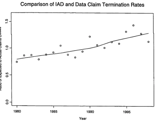
[image:42.539.126.398.367.583.2]

In this analysis, the “year” refers to the year of exposure (and claim termination). The results from Table 3.3 are displayed using a scatterplot along with a lowess smooth of the points in Figure 3.1 below.

Comparison of IAD and Data Claim Termination Rates

Figure 3.1: Comparison of Actual and Expected Experience over Time where expected experience is derived using the IAD89-93 table

(43)

evident. Is this a real improvement or, like the periods 1986 to 1988 and 1990 to 1992, merely a random fluctuation before the presumed underlying deterioration resumes its course?

Because of this very material change in aggregate experience over time, the results of the analyses by each of seventeen covariates are presented in a two dimensional form to show the experience over time as well as how it varies with the value for each individual characteristic. The only exceptions to this presentation style are experience by benefit size, age at claim, duration and year of policy commencement as the number of individual values for each characteristic are too great to allow such an exposition.

3.3.2 Summary of Results

Y e a r E x p e c te d A c tu a l I n d e x

1980 19 26 7 4 %

1981 79 92 86%

1982 2 2 6 261 87%

1983 515 651 7 9%

1984 629 715 8 8%

1985 76 3 8 2 6 9 2 %

1986 1202 1146 105%

1987 2 0 9 0 2381 88%

1988 2 1 4 2 2 5 8 0 83%

1989 2 3 5 2 2 5 1 3 9 4%

1990 3261 2681 122%

1991 4 8 9 5 4 6 2 5 106%

1992 5 1 4 8 5 0 8 2 101%

1993 6 4 4 7 5 7 3 6 112%

1994 6 9 6 0 6 3 6 9 109%

(44)

1996 8 1 6 6 5 6 5 8 144%

1997 7 4 9 0 5 8 6 2 128%

1998 5 4 7 7 4 8 3 0 113%

[image:44.539.112.421.344.742.2]

6 5 6 0 0 5 7 8 7 4 113%

Table 3.3: Comparison of Actual and Expected Experience over Time

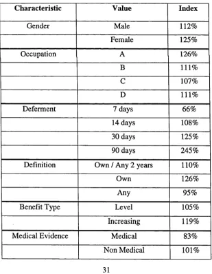
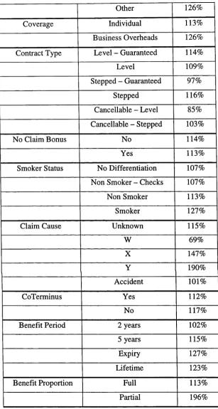
Table 3.2 shows the results for each characteristic presented as the Index for the total period ignoring differences by year. The experience by year for each characteristic is to be found in Appendix 3.2. This table identifies which values for which characteristics are material in impacting the termination experience.

Characteristic Value Index

Gender Male 112%

Female 125%

Occupation A 126%

B 111%

C 107%

D 111%

Deferment 7 days 66%

14 days 108%

30 days 125%

90 days 245%

Definition Own / Any 2 years 110%

Own 126%

Any 95%

Benefit Type Level 105%

Increasing 119%

Medical Evidence Medical 83%

(45)

O th e r 126%

C o v e ra g e In d iv id u a l 113%

B u s in e s s O v e rh e a d s 126% C o n tra c t T y p e L ev e l - G u a ra n te e d 114%

L ev e l 109%

S te p p e d - G u a ra n te e d 9 7 %

S te p p e d 116%

C a n c e lla b le - L ev el 85% C a n c e lla b le - S te p p e d 103%

N o C la im B o n u s N o 114%

Y es 113%

S m o k e r S ta tu s N o D iffe re n tia tio n 107% N o n S m o k e r - C h e c k s 107% N o n S m o k e r 113%

S m o k e r 127%

C la im C a u s e U n k n o w n 115%

W 69%

X 147%

Y 190%

A c c id e n t 101%

C o T e rm in u s Y es 112%

N o 117%

B e n e fit P e rio d 2 y e a rs 102%

5 y e a rs 115%

E x p iry 127%

L ife tim e 123%

B e n e fit P ro p o rtio n F u ll 113%

[image:45.539.110.417.45.620.2]

P a rtia l 196%

(46)

3.3.3 Some Initial Conclusions

The results summarised by Figure 3.1 and Tables 3.3 and 3.4 suggest that the characteristics used in IAD89-93 to predict claim termination rates, namely deferment, gender and occupation, do not capture significant differences in experience that are evident due to the presence of other rating factors. This suggests that the classification using the current industry table contains considerable heterogeneity. Indeed, usual industry practice in the application of the IAD89-93 table for Australian life insurers varies considerably. Some insurers apply a proportion (rating up or down) factor to the rates provided in IAD89-93. The proportion is calculated using a comparison of aggregate experience to the rates published in the IAD industry table. Other Australian insurers disregard the Australian table on the basis that it was constructed using insufficient experience. They instead base their rates on the CIDA85 tables produced in the United States and then apply a set of internally developed factors relating to age, smoker status and occupation class to bring the US table rates into line with the particular office experience.

In addition, not only is the experience deteriorating to an extent where IAD89-93 is materially overstating the likely termination rates, but also its shape for various characteristics may be materially and commercially significantly different to that shown in the experience.

3.4. GENERALISED LINEAR MODEL OF CLAIM TERMINATION RATES

3.4.1 Background to Generalised Linear Models

(47)

linear regression model, when used for the prediction of a dependent variable, Y (for example claim termination rate), with a number of independent variables, Xj, X2,....,Xp, (for example

occupation class, duration of claim, age, smoker status) can be described as follows:

1. A random component: each value of Y is normally distributed with expected value /u (which may depend on covariates) and constant variance a 1 2.

2. The systematic component: a set of independent variables Xj, X 2, ...,XP which combine to

p

produce a linear predictor rj given by 77 - ^ x fß r where the ßj are regression coefficients,

1

usually estimated by the least squares principle.

3. The “link” between the linear predictor and the mean of Y is n = t] The GLM extends this basic model in two significant ways:

(48)

2. The link function in (3) above can be any monotonic differentiable function. Common link functions include the identity link, the log link, the inverse link and the logit (or log-odds) link. The link function allows non-linearity in the relationship between Y and the covariates.

Having fit a GLM, the process of determining whether predictors are adding value to the model is also different to the process used in multiple regression or traditional linear modelling, insofar as the so-called deviance is used as a measure of fit rather than the more traditional “variation- explained”.

To assess the adequacy of the fit of a GLM we need to define the deviance statistic. The deviance reflects the discrepancy between the actual values of the dependent variable and the fitted values relating to the dependent variable in a likelihood sense. The formula for the deviance is

The deviance is the scaled difference in log-likelihoods between a perfectly fitting (or saturated) model and the model for which the deviance is being calculated.

(3.1)

where (f) is the dispersion parameter and i(y ,</)^ is the log-likelihood function for the observed

(49)

The addition of independent variables to a GLM inevitably reduces the deviance. The amount of this reduction in deviance (in other words the size of the step taken towards the perfectly fitting model) may be used as a measure of whether that particular independent variable should be retained in the model.

3.4.2 Advantages of Using Generalised Linear Models for Claim Termination Rates

Some advantages of using GLMs in describing termination rates are that:

• they enable the impact of changing the level of a rating factor to be quantified in a way that does not consider the change in other rating factors that will accompany such a change in rating variable. For example, the 1997 Disability Report considers the impact of occupation class on claim duration. The report states that claim duration for occupation class A is longer than that for occupation classes B to D. The GLM enables you to isolate out the impact of the change in occupation class from the changes in other variables which occur when you move from occupation class A to D. For example females are rarely in occupation class D, and secondly occupation class A lives are usually more severely disabled before they are unable to work than is the case for, say, occupation D lives; note, however, that such interpretations may struggle fo find real- world analogues, as changes in individual covariates often occur.

(50)

• they enable suitable modelling of the variance of the expected termination rate (unlike conventional linear modelling) to more adequately reflect real-world experience;

• the predicted termination rates vary smoothly meaning that premiums and reserves calculated from the model will also vary smoothly for continuously varying covariates. They won’t necessarily be smooth for, say, binary covariates.

• the results for termination rates can be summarised as the result of a single model rather than through the provision of a large set of different tables. This compactness allows for easy calculation and also provides a very efficient means of communicating such information.

3.4.3 Discussion

The GLM fitted in this research used data from the whole period 1980 to 1998 but using only a limited set of characteristics in order to facilitate the actual calculations by reducing the number of cells analysed. A GLM fit to the full set of characteristics using only data from the latest data period, 1995 to 1998, has been derived for claim incidence rates. The results of this analysis are shown later in this chapter.

(51)

A number of different GLMs were fit to the termination rate data. After considerable experimentation and assessment of residual plots, it was decided that the Poisson error structure was the most appropriate for describing the mean-variance relationship inherent in the data. It was comforting to note that this error family is the same one commonly used for claim frequencies when the claims experience of many short-tail lines of general insurance business are modelled.

The data selection for the final GLM chosen used claims which had a deferment of 14 or 30 days, did not have an Unknown claim cause and had Individual coverage. There were 83,000 such claims with 675,000 months of exposure. The following characteristics were retained in the final model:

Rating Variables Rating Variables

Definition Claim Cause

Gender Deferment Period

Occupation Class Benefit Rate Smoker Status Year of Exposure

Age at Claim Claim Duration

Table 3.5 Retained Covariates

There were 275,000 cells in the data, after allowing for all multi-way classifications of the above ten rating variables.

(52)

In order to give greater weight to those observations in which we have more confidence in, the GLMs were fit using the exposure for each rating factor combination as weights in the fitting algorithm.

The results in Appendix 3.3 show that all of the following rating factors aid significantly in the modelling of termination rates: age at date of claim, cause of claim, duration of claim, gender, occupation class, smoker status, deferment period, benefit rate and the calendar year at the date of possible claim termination. In addition a significant duration and age interaction was found. The dataset includes all claim terminations so that at every possible duration only certain claims will actually be observed to terminate.

From the output in Appendix 3.3, we can calculate the fitted values for claim termination rates. The prediction formula is

Fitted Claim Termination Rate = exp(32.3 .008AgeClaim + 0.371(ClaimCauseW) + ... -.00652(AgeClaim*Sqrt(Duration)))

Standard errors of the fitted coefficients are provided in Appendix 3.3. It is clear from Appendix 3.3 that the model retains a significant residual deviance. This result is not surprising given that the nineteen years of data was included in the analysis and only a limited number of rating factors were included as explanatory variables. The interpretation of deviance residuals is explained in McCullagh (1989). A number of other variables and transformations of existing variables have been explored in the context of claim incidence rates.

(53)

model for claim termination rates (and incidence rates) based only on the most recent five years of claim data. This reduced dataset will allow a considerably improved fit to the data to be achieved than was possible in the full analysis.

Other interesting results of the analysis include:

• The benefit rate has a statistically significant, negative impact on the rate of claim termination;

• there is a statistically significant interaction between duration and deferment period in determining the termination rate. At shorter durations the predicted termination rate is significantly higher for the shorter deferment period. After durations of approximately 8 months this difference becomes non-significant;

• there has been a statistically significant decline, over time, in termination rates when aggregated across all levels of the rating factors. The decline in termination rates is still statistically significant even after the impact of all other rating factors has been allowed for.

(54)

3.5 STOCHASTIC CLAIMS RESERVING

Using the GLM output shown in Appendix 3.3, we aim to find the approximate distribution, using simulation, of the required reserves in respect of a DII portfolio to ensure relevant probabilities of adequacy. The analysis is for the average of 100 claims that are new at the date of valuation with a monthly disability payment of $2600. The graph below was generated for the case of a male aged 40, in occupation class A, with a deferred period of 2 weeks who became disabled because of an accident.

Reserve Requirements for $2600 Monthly Claim at Duration Zero

[image:54.539.101.430.303.563.2]

Percentage

Figure 3.2: Reserve Requirements to obtain varying probabilities of adequacy

In the above analysis, allowance has been made for deteriorating claim termination rates and for interest at 6% per annum, compounding continuously.

(55)

distributed. This is because the fitted value is a linear combination of coefficient estimates and constant covariate values and the coefficient estimates are maximum likelihood estimates, which are themselves asymptotically normally distributed. The delta method was used to approximate the variance of the actual fitted values for the termination rates. The number of terminating claims, given the termination rate, was then simulated from a binomial distribution.

Table 3.6 shows the reserves required to give a particular probability of the reserve being adequate using the simulation approach described above.

Probability Claim Reserve at Start of Claim

Increase Over 50%

50% 33,764

75% 36,749 9%

90% 39,692 18%

95% 41,180 22%

99% 45,357 34%

Table 3.6: Reserve Requirements by Probability of Adequacy

The reserve calculated using a traditional deterministic approach would be approxiamtely at the 50% probability level in Table 3.6.

3.6 A GLM for Claim Incidence Rates

(56)

E [log (Y)] = log(exposure) + /?0 + ^

A*;+ X A

x ix j * (3.2)

7=1 selected i,j',k=\

where Y denotes actual number of claims multiplied by benefit percent, the Xj are covariates associated with holders of DII contracts and the ß } are regression coefficients derived using

maximum likelihood estimation (McCullagh and Neider (1989)). The exposure is the amount of time that disability income insurance holders are exposed to the risk of becoming disabled and is recorded in days. The xpCj terms are interaction terms. These will be discussed further in this section.

This model is fit using an offset for log(exposure). The offset ensures that the model is fit with a regression coefficient for log(exposure) equal to one. This means that the model can be rewritten as

£(log(lncRate)) = ,#0 + V /?.*,.+ £ A x ix j * (3-3)

7=1 selected i, j, k = \

where IncRate denotes the incidence rate of claims measured on a per day basis.

(57)

C o v a ria te C o e ffic ie n t

E s tim a te

Z -S c o re C o v a ria te C o e ffic ie n t

E s tim a te

Z -S c o re

G e n d e r 0 .2 7 4 7 4 5 2 .9 3 B e n a m o u n t6 0 .2 1 1 6 4 1 6 .1 0

A g e 0 .2 4 6 0 1 5 15.81 B e n a m o u n t7 0 .2 5 4 1 9 9 5 .5 2

V A §e -2 .3 1 0 6 9 7 -1 8 .6 3

S m o k e r 0 .1 5 6 6 8 5 10.61

O c c u p a tio n B 0 .9 2 1 9 4 4 7 .4 9 A id s 0 .2 2 2 8 7 9 1 5 .0 4

O c c u p a tio n C 1 .8 0 5 0 6 1 2 2 .7 7 D u r a tio n l 0 .2 0 7 5 7 3 1 2 .5 6

O c c u p a tio n D 2 .0 0 0 9 9 9 2 3 .5 7 D u ra tio n 2 0 .0 8 3 4 7 7 5 .8 9

D e fin itio n 2 -0 .0 5 8 8 7 1 -4 .0 3 N e b 0 .0 6 7 3 6 7 4 .6 9

D e fin itio n s - 0 .0 4 3 3 1 9 -0 .8 9 C o n t r a c t - 0 .3 2 1 5 3 2 -4 .7 6

D e fin itio n 4 -0 .2 1 9 7 1 3 -4 .5 8 C o n tra c t2 - 0 .0 7 8 0 4 0 -3 .9 9

D e fin itio n s -0 .3 5 6 4 3 1 -8 .8 6 C o n tra c t3 0 .1 4 9 0 4 5 3 .0 6

D e fin itio n s - 1 .1 5 8 2 6 8 -1 .4 6 M e d ic a l -0 .2 0 5 6 1 7 -6.11

D e fe rm e n t2 0 .9 0 6 2 2 1 1 .2 0 A g e * O c c u p a tio n B - 0 .0 0 9 2 1 9 -3 .3 8

D e fe rm e n t3 - 0 .0 4 8 2 2 2 -0 .0 6 A g e * O c c u p a tio n C - 0 .0 1 9 7 5 2 -1 1 .3 9

D e fe rm e n t4 -2 .5 4 0 3 5 5 -3 .0 9 A g e * O c c u p a tio n D -0 .0 2 1 1 8 2 -1 1 .4 2

D e te rm e n ts - 2 .6 1 2 0 5 5 -3 .2 0 G e n d e r* A g e 0 .0 0 4 8 7 0 2 .4 0

(58)

D eferm en t7 -3 .5 3 3 4 3 8 -1 .5 2 G ender*O ccupationC -0 .4 7 4 0 7 4 -9 .7 3

D eterm en ts -3 .3 3 3 8 0 2 -6 .7 2 G ender*O ccupationD -0 .5 6 3 5 2 9 -7 .0 8

B en p eriod l -1 .0 7 8 8 5 4 -1 3 .6 2 A ge*D eferm ent2 -0 .0 2 5 9 2 0 -1 .9 6

B en period 2 0 .0 1 9 6 2 8 8 1.3 9 A ge*D eferm ent3 -0 .0 2 3 0 9 7 -1 .7 5

B en am ou nt2 0 .0 4 4 0 5 4 2 .2 0 A ge*D eferm ent4 0 .0 1 1 8 8 1 0 .8 0

B en am ou n t3 0 .1 7 4 3 7 8 9 .0 6 A ge*D eferm ent5 0 .0 0 2 8 7 7 0 .2 0

B en am ou n t4 0 .2 0 0 4 3 0 9 .8 8 A ge*D eferm ent6 0 .0 2 7 7 2 0 1.08

[image:58.539.43.487.47.339.2]

B en am ou n t5 0 .2 3 5 9 0 0 8 .7 3 A ge*D eferm ent7 -0 .0 1 1 8 6 0 -0 .2 5

Table 3.7 Incidence Rate GLM Coefficients

The above table shows that thirteen interaction terms are included in the model for claim incidence rates. Interaction terms add to the flexibility of the model and enable a more realistic description of the underlying data. To consider an example, we see in the above table that the gender by age interaction is statistically significant. This means that the impact of age on incidence rates is different dependent on the value taken by gender in the model. The gender by age interaction term has a positive coefficient meaning that for a unit increase in age the resulting predicted incidence rate increases more when gender is 1 (female) than when gender is 0 (male).

(59)

ensure that this proportional increase in variance with the fitted values was a reasonable assumption for this data. The test indicated that there was no evidence of overdispersion.

Another important characteristic of this analysis was the treatment of the smoker variable. In the original data, approximately 3.5% of the exposure was not classified as either smoker or non- smoker. One approach to the modelling is to ignore this 3.5% of the data. It is not possible to fit the GLM using a subset of the required covariates for certain data points unless a specific imputation technique is put into place. One imputation method is, therefore, to attempt to predict the value of the missing smoker value by employing logistic regression with smoker as the response. This analysis fits a regression model where the response variable is the probability that the policyholder was a smoker and the explanatory variables are the other covariates including claim information available in the data. The logistic regression methodology ensures that the fitted values for the probability of being a smoker are on the range from 0 to 1 and hence can be used as valid covariates in the fitted GLM.

3.7 Comparison of GLM Results with IAD89-93

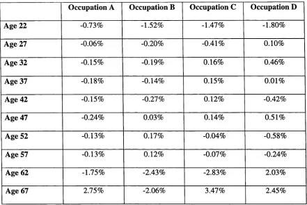
An analysis of the main differences between both the smoothed incidence rates, fitted by the GLM from Section 3.6, and the existing rates from IAD89-93 is given in this section.

(60)

Occupation A Occupation B Occupation C Occupation D

Age 22 (IAD) 1.8889% 4.0643% 5.4911% 5.7715%

Age 22 (GLM) 1.6661% 3.3402% 6.4850% 7.5635%

Age 27 (IAD) 1.7401% 3.4906% 4.9069% 5.3417%

Age 27 (GLM) 1.5625% 2.8803% 5.4560% 6.2806%

Age 32 (IAD) 1.8441% 3.2985% 4.8465% 5.4489%

Age 32 (GLM) 1.6318% 2.8408% 5.1082% 5.8771%

Age 37 (IAD) 2.1474% 3.4744% 5.1656% 5.9374%

Age 37 (GLM) 1.8429% 3.0734% 5.2040% 5.9217%

Age 42 (IAD) 2.6645% 4.0039% 5.8266% 6.7658%

Age 42 (GLM) 2.1955% 3.5029% 5.5956% 6.3472%

Age 47 (IAD) 3.4226% 4.8797% 6.7981% 7.8987%

Age 47 (GLM) 2.7603% 4.1802% 6.2835% 7.0909%

Age 52 (IAD) 4.4471% 6.1014% 8.0550% 9.3069%

Age 52 (GLM) 3.6175% 5.2749% 7.4288% 8.3044%

Age 57 (IAD) 5.7930% 7.6759% 9.5784% 10.9671%

Age 57 (GLM) 4.9656% 6.6699% 8.9480% 10.1073%

Age 62 (IAD) 7.5205% 9.6170% 11.3560% 12.8620%

Age 62 (GLM) 7.0301% 8.8306% 11.2966% 13.0054%

Age 67 (IAD) 9.4457% 11.7093% 13.2333% 14.8477%

Age 67 (GLM) 10.2979% 12.4523% 14.8078% 17.2813%

(61)

Table 3.9 compares the smoothed incidence rates using the GLM from Section 3.6 and the rates from IAD89-93 for the one-month deferment period policies.

Occupation A Occupation B Occupation C Occupation D

Age 22 (IAD) 0.5856% 1.1248% 2.2204% 2.2662%

Age 22 (GLM) 0.6874% 1.3810% 2.6977% 3.2659%

Age 27 (IAD) 0.5358% 1.0037% 1.9808% 2.1374%

Age 27 (GLM) 0.6578% 1.2108% 2.2889% 2.7232%

Age 32 (IAD) 0.5947% 1.0333% 1.9486% 2.1758%

Age 32 (GLM) 0.6861% 1.1913% 2.1743% 2.5688%

Age 37 (IAD) 0.7290% 1.1581% 2.1002% 2.3628%

Age 37 (GLM) 0.7853% 1.2686% 2.2314% 2.6056%

Age 42 (IAD) 0.9400% 1.3428% 2.4340% 2.7153%

Age 42 (GLM) 0.9504% 1.4557% 2.4194% 2.8215%

Age 47 (IAD) 1.2517% 1.6247% 3.0144% 3.3107%

Age 47 (GLM) 1.2068% 1.7347% 2.7519% 3.1868%

Age 52 (IAD) 1.6995% 2.1345% 3.9507% 4.2741%

Age 52 (GLM) 1.5995% 2.1383% 3.2830% 3.7740%

Age 57 (IAD) 2.3454% 3.0658% 5.4235% 5.7822%

Age 57 (GLM) 2.2051% 2.7362% 4.0876% 4.6466%

Age 62 (IAD) 3.2603% 4.6743% 7.6233% 8.0478%

Age 62 (GLM) 3.1133% 3.4621% 5.1661% 5.9687%

Age 67 (IAD) 4.3157% 6.5442% 9.9974% 10.6651%

[image:61.539.44.479.99.669.2]

Age 67 (GLM) 4.4394% 4.6979% 6.9509% 7.4860%

Actuarial models for the analysis of disability income insurance