Tracer diffusion in liquids

by

John f . Tilley.

Thesis for the Degree of Master of Science

Australian National University Diffusion Research Unit

This w ork is divided into two se c tio n s. The f i r s t d e ta ils the m e a su re m e n t of in trad iffu sio n co efficien ts by conventional d ia p h ra g m -c e ll technique. Iso to p ic frictio n co efficien ts have been calcu lated fro m th e in trad iffu sio n , m utu al-d iffu sio n , and activ ity d ata fo r th e sy ste m s; Sucrost la b elled s u c r o s e -w a te r and M an n ito l-lab elled m a n n ito l-w a te r. An attem p t h as been m ade to c o rre la te fric tio n co efficien ts w ith m o le c u lar p ro p e rtie s . B ecau se of th e lim ited data av ailab le fo r s y ste m s of th e type studied good c o rre la tio n s w ere not obtained.

The second section d e s c rib e s th e developm ent of a continual m o n ito rin g technique applied to the d iap h rag m c ell. In an e ffo rt to im p ro v th e a c c u ra c y of th is technique a la rg e n u m b er of tr a c e r - io n concen tratio n m e a su re m e n ts w e re m ade on th e sy ste m S trontium c h lo rid e - w a te r. The r e s u lts obtained fro m continual m on ito rin g w e re co m p ared w ith th o se from

n

t

CONCLUSION

C o rre la tio n of fric tio n co efficien ts with m o le c u la r p ro p e rtie s is e m p iric a l a t p re s e n t. In fu tu re, stu d ie s should be u n dertaken on

hom ologous s e r ie s of so lu tes to enable e a s ie r c o rre la tio n than i s p o ssib le a t p r e s e n t. The w ork done on the continual m o n ito rin g technique in d ic a tes th a t th e m ethod w ill p ro v id e highly a c c u ra te diffusion co efficien ts if

Page CHAPTER 1

INTRODUCTION 1

Liquid diffusion 2

Definitions 4

Methods for measuring tracer-diffusion coefficients 5 Theory of tracer-diffusion in electrolyte solutions 11

Tracer diffusion of non-electrolytes 12

Multicomponent diffusion 14

CHAPTER 2

THE DIAPHRAGM CELL METHOD 18

Theory 19

Stirring of solutions 20

Transport mechanisms 21

Diaphragm steady state 22

Volume change on mixing 23

Cell calibration 24

Duration of experiments 32

Cell constant variation 33

CHAPTER 3

INTRADIFEUSION MEASUREMENTS IN SOME AQUEOUS NON-ELECTROLYTE

SYSTEMS. THEORY AND EXPERIMENTAL 35

Experimental flow equations 37 Relation "between intradiffusion coefficient and mutual-

diffusion coefficient 38

Theoretical flow equations 40

Listing of the auxiliary data required for the calculation

of friction coefficients 44

Treatment of the data 47

Reagents 30

Purification of radioactive compounds 52

Preparation of solutions for diffusion 53

Preparation of solutions for counting 55

Determination of radioactive tracer concentration 55

Counting technique 56

CHAPTER 4

INTRADIFFUSION MEASUREMENTS IN SOME AQUEOUS NON-ELECTROLYTE

SYSTEMS. RESULTS

AND

Experimental intradiffusion coefficients 61

Discussion of errors 63

Special effects 64

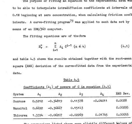
Curve fitting the experimental data 66

Comparison of intradiffusion data with other related data 67

Eriction coefficients 73

CHAPTER 5

CONTINUAL MONITORING- METHOD OP MEASURING DIFFUSION

COEFFICIENTS. THEORY AND EXPERIMENTAL 78

Aims o f th e s e m ic o n d u c to r m o n ito r in g m ethod 79 D e te c to r c h a r a c t e r i s t i c s 80

D e te c to r n o is e 81

R e q u ire m e n ts o f a s s o c i a t e d e l e c t r o n i c eq u ip m en t 83

Use o f d e t e c t o r s 84

C om parison o f se m ic o n d u c to r d e t e c t o r s w ith o t h e r r a d i a t i o n

d e t e c t o r s 86

D esig n o f th e d i f f u s i o n c e l l 87 C hoice o f s u i t a b l e is o t o p e s 88 P u r i f i c a t i o n o f r a d i o a c t i v e s tr o n ti u m c h l o r i d e 89

E x p e rim e n ta l p r o c e d u r e 90

C a l c u l a t i o n o f d i f f u s i o n c o e f f i c i e n t 91

C o u n tin g c o r r e c t i o n s 92

CHAPTER 6

CONTINUAL MONITORING METHOD OF MEASURING DIFFUSION

COEFFICIENTS. RESULTS AND DISCUSSION 93

T r a c e r - d i f f u s i o n c o e f f i c i e n t s o f s tr o n ti u m io n i n

s tr o n tiu m c h l o r i d e s o l u t i o n s 94 C om parison w ith p r e v io u s d a t a

Limitations of the measuring system 9&

Problems in background estimation 98

Estimation of x> rediffusion time 100

Conclusion 101

1 2 3 4 5

6

8

85

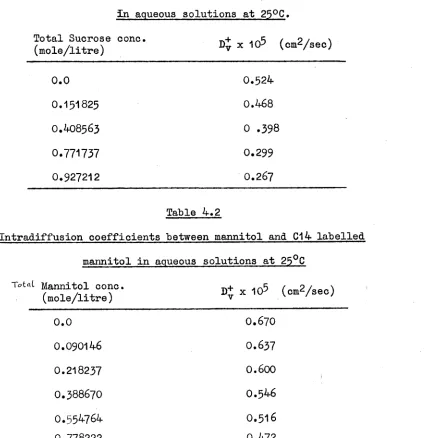
Diffusion of Sucrose in aqueous solutions

Diffusion of mannitol in aqueous solutions

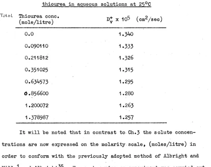
Intradiffusion coefficients of thiourea

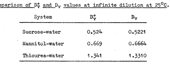
Comparison of diffusion data of sucrose

Test of equation 4.4 for thiourea

Friction coefficients of sucrose

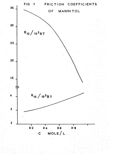
Friction coefficients of mannitol

Cross-section of a surface-barrier detector

Circuit of detector system

Diaphragm cell for continual monitoring

CHAPTER 1

Liquid diffusion

It has been customary to express molecular interactions in diffusing liquid systems in terms of the diffusion coefficients of the components. Recently, a number of workers have suggested that data from diffusion studies might be more informative if transport properties were expressed in terms of friction coefficients. The

calculation of reasonably precise isotopic friction coefficients requires highly accurate mutual-diffusion, tracer-diffusion and activity data. Over the past two decades several techniques have been introduced for the measurement of tracer-diffusion coefficients in liquids, and the most accurate of these is the diaphragm-cell method. Present practice is to calculate a diffusion coefficient from just two measurements of the tracer concentration all made at the conclusion of the experiment. In spite of this limitation, pre­ cision of the order of a few tenths of is possible1 * Part of the work described in this thesis is devoted to measuring tracer diffus­ ion coefficients by the above method and thereby to calculate frict­ ion coefficients. In addition;with the aim of enhancing the accuracy of the method, a project was undertaken in which a large number of tracer-concentration measurements were made during the course of an experiment.

driving force. Onsager^, when deriving equations for diffusion, used the gradient of chemical potential-* as the force. For tracer diffusion this gradient is considered to be a term derived from the entropy of mixing. An established method for measurement of tracer- diffusion coefficients is by means of radioactive isotopes. It is assumed that the diffusive behaviour of labelled and unlabelled isotopes is identical. A feature of diffusion in aqueous solution is that the diffusing entity is usually hydrated, and since diffus- ional velocities are more dependent on size than mass, the substit­ ution of a labelled atom in place of an unlabelled one is virtually

4

unnoticeable. Most experimenters have found that diffusion coeffic­ ients for the same molecule measured with different labelled isotopes are identical within the precision of measurement, except where mass differences are large.

The equations derived by Fick^ are the basis of diffusion measurement. The first law states that for an isothermal single­ phase system the diffusional flux (j) passing at time (t) through unit area perpendicular to the x- direction is proportional to the

concentration

(c)

independent of concentration in the above equations and is actually s

the case for tracer-diffusion. The second law applied to all diff­

using systems and a solution of it, subject to the appropriate

boundary conditions is employed in both free-diffusion and

restricted-diffusion studies. The first law may be applied to simpler systems

where the concentration gradient is tirne-independent. This situation

is closely approximated in the diaphragm-cell method.

Definitions.

Some confusion has been evident in the past in regard to the

terminology used to describe the various types of diffusion coeffic­

ients. An explanation of the various terms used in this work is given.

Tracer diffusion is a general term describing the motion subject

to a concentration gradient of a labelled component present in (very)

low concentration in an otherwise uniform medium. One aspect of

tracer diffusion is where the tracer species has a chemically ident­

ical counterpart in the supporting medium. This has been termed

intradiffusion^. A special case of intradiffusion is self diffusion,

where the supporting medium contains only the chemically identical

counterpart of the tracer. In a diffusing system of two chemically

b t r\

rKr^J

different components several different mtrb^ai^hiffusion coefficients

exist, depending on the frame of reference chosen. The mutual-diffus­

for the volume-fixed frame of reference. In this case the

mutual-diffusion coefficients of each component are identical. Also, if

no volume change occurs on mixing, the cell-fixed and volume-fixed

frames of reference coincide.

Methods for measuring tracer-diffusion coefficients.

Open-ended capillary method.

This method was developed for aqueous solution work by Anderson

and Saddington^ in 1949. Modifications have been carried out by Wang"'7,

Mills^, and Mills and G-odbole^. The theory of the method has been explained by these authors.

Capillaries used are approximately 2 cm in length and 0.5 mm

internal diameter and sealed at one end. The tube is filled with

tagged solution and immersed in a relatively large reservoir of in­

active solution, of the same chemical composition. Diffusion is

allowed to proceed and after a measured time interval the quantity

of tagged material remaining in the capillary is measured and com­

pared with the initial quantity. It is possible to diffuse tracer

solution into the capillary by filling the bath with tagged solution

and the capillary with inactive solution. Solution of kick's second

law for the given boundary conditions produces a relatively simple

equation if the experimental diffusion period is sufficiently long.

Errors in capillary method.

The capillary equation shows that the method is an absolute

one, but it suffers from some degree of uncertainty in the exactness

invariably results in a slight scooping out of tracer solution.

A drop of liquid is usually left on top of the open end to minimise

10 i i

this error. Mills and Kennedy , and Mills and Adamson'1, showed

that losses of approximately 1.5% of the capillary contents resulted

under stirred conditions, corresponding to a lengthening of the diff­

usion time by 100 seconds. This is negligible when compared with

usual diffusion times of 2 x 1 (ß seconds.

Solution of F i c k ’s second law requires that the concentration

of the tracer at the open end of the capillary is zero. Consequently

some form of stirring is necessary to remove the stagnant layers of

c -ip

tracer solution. Anderson and Saddington , Burkell and Spinks ,

13

Matuura and Shimozawa and several others, neglected stirring, and

their results would tend to be lower than the true value. Wang?

attempted to remedy the defect by using a one litre reservoir and

stirring solutions with a large paddle placed below the capillary.

However because of the turbulence caused by the paddle, the diffus­

ion coffecients were higher than the true value. Tagged solution

was being scooped out of the capillary by the uneven flow of reserv­

oir solution over the mouth of the capillary. Quoted experimental

error of the method at this stage was ± 2/o.

Further study of the technique by Mills and K e n n e d y ^ indicated

possible additional errors due to ion adsorption of the tracer, and

pH differences between tracer and bath solution. The next advance

flow of reservoir solution was passed over the open end of capill­

aries. The flow rate of reservoir solution was varied until results

from the capillary cell and diaphragm cell agreed. The accuracy

claimed was ± 1$.

The results of Mills and G-odbole^ using a continual monitoring

method indicated a precision of + 0.2$. In this method the capillary

containing tracer solution was placed inside a plastic scintillator

mounted on a photomultiplier tube, and. enabled a continuous determin­

ation of the activity remaining in the capillary. By using low conc­

entrations o1 solute they were able to test the Onsager^ limiting law

for ionic diffusion.

Free diffusion.

f.ang and Kennedy^ + used large tubes of 0.1cm diameter, which

were divided into three sections. The duration of the experiment

was such that the change in solute concentration at the closed end

was negligible, and a solution of F i c k ’s second law for the approp­

riate boundary conditions allowed the diffusion doefficient to be

found. Claimed accuracy of this method was ± 1

$.

Porous-Frit method.

A thin porous disc (thickness 0.033 to 0.1~]b- cm, hole diameter

1p) of inert porcelain is saturated with labelled solution and then

suspended in a large bath of unlabelled material. From the rate of

decrease of activity with time the diffusion coefficient is calculated.

diffusing polymers. They suspended a porcelain disc saturated with the solution of interest from the arm of an analytical balance and determined the diffusion coefficient from the time rate of weight change. The bath liquid was stirred except when recording weights. The pore size of the frit was chosen to eliminate bulk flow and wall effects.

As with the open-ended capillary cell immersion errors are present but are insignificant for sufficiently long diffusion times. Errors are likely due to diffusion from the ends of the frit and

scooping-out of tagged solution may well occur because of the turb­ ulent stirring employed. In an extension of the method Marcinkowsky et al17 used the following procedure : a porcelain frit was saturated with radioactive tracer solution, and a non-labelled solution of the

same chemical concentration was pumped past the frit. The diffusion coefficient was found from a plot of counting rate against time together with frit calibration data. They calibrated the frit with the data of Mills^ for tracer diffusion of Na+ in 1M EaCl and adjusted the flow rate of the bulk solution so that their results coincided with calibration data. They found that for best results frits had to be aligned parallel to the direction of flow. Accuracy claimed was ± 5%«

Diffusion coefficients in molten salts1^ have been determined by the porous-frit weight-loss method. Results obtained have been

Diaphragm cell method.

In 19-4-7 Adamson5^ adapted the diaphragm cell for tracer diffusion measurements. Previously it had been used for mutual- diffusion studies. Diffusion is confined to the sintered glass diaphragm separating the upper and lower cell compartments. One compartment is filled with tracer solution and the other with iso- topically normal solution of the same chemical concentration. Sol­ utions are stirred continuously and sampled at beginning and end of experiments. Being a pseudo-steady state method a solution of Pick’s first law is used. Cells are calibrated with accurate mutual-diffus­ ion data (± 0.1%) obtained by optical techniques and the method gives diffusion coefficients reproducible to approximately + 0.3%« Several sources of error exist, viz. ion adsorption and stirring speeds.

Nielsen, Adamson and Cobble^0 , and Stokes^ found that measure­ ments below 0.05M for univalent salts were in error, due to adsorpt­

ion of ions on the glass sinter. The formation of an electrical double layer contributes to total transport by surface diffusion. This then excludes the method for testing the limiting laws of elect­ rolyte theory.

20

field argued that solutions were stirred by density difference and while this may have applied (for mutual diffusion) to the bulk of solution, the existence of stagnant layers on the diaphragm was realised from studies of reactions at solid—liquid interfaces» Several methods of stirring were employed, but for the most part they were not satisfactory. Stokes^ indicated a successful method whereby small glass rods containing iron wire sweep the diaphragm at 50 to 80 r.p.m. One just sinks in the upper solution and one just floats in the lower solution.

Theory of tracer diffusion in electrolyte solutions.

Onsager and Fuoss2^ formulated a general equation expressing

the diffusion coefficient of an ion in terms of the solution conc­

entration and mobilities of the ions present. Onsager2 extended

the theory to obtain a limiting law. This law expressed the diff­

usion coefficient of an ion present in low concentration in terms of

the electrolyte concentration and conductances of the ions.

Gosting and Harned25 gave a simpler version of the law which

could be used to test experimental data. The law applies only to

very dilute solutions. The form of the limiting law is as follows:

D = D0 - K C1^2

where D is the tracer-diffusion coefficient of the ion under study.

% value of the tracer-diffusion coefficient at infinite

dilution given by Nernst equation.

K is a constant involving a number of thermodynamic properties

of the solution and

C is the concentration of the supporting electrolyte.

The limiting law has been confirmed by the measurements of

Mills and G-odbole^. A semi-empirical extension2^ of the limiting

law has enabled reasonable correlation between theoretical and

experimental data for a slightly larger concentration range (up to

0.1 M). The extension has been to include a factor including the

ion size, which is neglected in the original treatment. The estim­

concentrations greater than 0.1M is empirical in the absence of any

suitable theory to account for the complex phenomena occurring at

these concentrations.

A relation between diffusional mobility and viscosity has been

obtained and is expressed in the Stokes-Einstein equation. However

the non-applicability of this equation to the aqueous tracer diffus­

ion considered here is not surprising since the relation was derived

for large uncharged solutes in non-polar solvents. Because of the

highly polar nature of water and the charges on ions there is a certain

structure present and the idea of local viscosities near ions being

larger than the bulk viscosity has been discussed by Wang^7. Empir­

ical extensions have been derived from Onsager's equation to take

account of viscosity and hydration and ionic charge, but have not on

the whole been successful in accurately predicting the experimental

data.

Tracer-diffusion of non-electrolytes.

Theories relating mutual and tracer-diffusion coefficients in

binary liquid mixtures are of two general types.

Adamson*^ and Hartley and Crank^9 propose that the mutual-diffusion coefficient is equal to the tracer-mutual-diffusion coefficient

multiplied by an activity correction term.

w h e r e )^cr^ i s a r e s i s t a n c e c o e f f i c i e n t a n d i s t h e m o le f r a c t i o n o f

c o m p o n e n t i , i s t h e a c t i v i t y o f c o m p o n e n t 1 a n d D-j 2 i s t h e m u tu a l'

d i f f u s i o n c o e f f i c i e n t o f c o m p o n e n t 1 i n c o m p o n e n t 2 .

C arm en a n d S t e i n o b t a i n e d

»12 = (N2D* + N ^ X ^ l n a i ) a I n N>,

b y s a y i n g t h a t _{N <r|>v}RT

A dam son o b t a i n e d t h e s i m i l a r e x p r e s s i o n

D12 = ( + *2*1) ( )

b e i n g t h e v o lu m e f r a c t i o n o f c o m p o n e n t i , a n d D* t h e t r a c e r - d i f f u s i o n

c o e f f i c i e n t o f c o m p o n e n t i .

I r a n i a n d A d am so n -^ , B e a r m a n 3 2 , a n d Laram-^ u s e t h e c o n c e p t o f

f r i c t i o n c o e f f i c i e n t s b e tw e e n e a c h o f t h e d i f f u s i n g m o l e c u l e s t o

p r e d i c t i n t e r - r e l a t i o n s b e tw e e n m u t u a l a n d t r a c e r - d i f f u s i o n c o e f f i c i e n t s .

xx

The e q u a t i o n s o f L am nr^ c o n t a i n q u a n t i t i e s w h ic h c a n n o t b e

d e t e r m i n e d e x p e r i m e n t a l l y b u t a n a p p r o x i m a t i o n w h ic h may b e u s e d i s

D / j 2 — N - j

Dj . Dg0 D*° -

$

~b I n a2

b l n C2

Irani and Adamson’s approximate relation is ä ln &2

»12 = (»2 -

I S A ) / 01 - alTcJ

where ^ is the solution viscosity,^ ^ the viscosity of pure 2.

Bearman's equation for regular solutions is

D* / D| = V2 / V1

wh ere is the partial molar volume of component 1.

Bearman32 and M i l l s ^ have considered the range of applicab­ ility of the preceeding equations, and stated that the equations should apply only to regular solutions. However M i l l s ^ added that study of the interactions of like molecules as a function of conc­ entration may lead to an extension of the statistical mechanical equations of Bearman-^ to non-regular systems.

Multicomponent diffusion.

will enable the liquid state to be better understood than is the case at present.

Isothermal diffusion in multicomponent systems may be des­ cribed by either of two types of formulation. The method developed by G-osting^^ based on Fick’s laws uses diffusion coefficients to relate diffusional flux and concentration gradients. For a system of n non-reacting components, the flux of component i measured with respect to a frame of reference R is given by

n ^

Cfc-(Ji)R = - E (°ik)R k=1

(i = 1,2 ... n)

D ± ± are termed main term and cross-term diffusion coeffic­

ients, the ik denoting the effect on the i th ion of the flow of the k th ion.

The frame of reference^ R may refer to the volume-fixed, cell-fixed, mass-fixed or number-fixed frames of reference.

For the case of tracer diffusion the experimental data is ob­ tained on the cell-fixed frame of reference which coincides with the volume-fixed frame as there is negligible volume change on mixing the diffusing components.

of most of the experimenters was to confirm the Onsager Reciprocal

Relations.

ffor a large number of irreversible phenomena it has been found

that the flows are linear functions of the thermodynamic forces in­

v o l v e d ^ . This may be expressed as

n

- (Ji)R

(i = 1 ,2 ... n)

where the force producing diffusion Xk is assumed to be the chemical

potential gradient of the k th component. The (Lj_k )R are termed

phenomenological coefficients. Their magnitudes depend on the frame

of reference chosen.

Woolf, Miller and G o s t i n g ^ have given a rigorous derivation

of the relations between (Lik )R and (i>ik )R coefficients. They showed

that by making all forces and flows independent, the phenomenological

coefficients will obey the Onsager Reciprocal Relation expressed in

an appropriate form e.g.

(R ik)v = (^ki)v (i / k )

where v indicates the volume-fixed frame of reference.

By using a different starting point a set of transport coeffic­

ients independent of the reference frame may be defined. Onsager

used the relation

X± = ^ R ik • Jk (k = 1 >2... n )

and implying

Rik

= Rki

(i / k)

The flux Jp may be expressed in terms of the velocity vp of the

i th component by

(Ji)R

Laity^5, KleranA^, B e a r m a n ^ and D u n l o p ^ have derived equations based

on the equation of Onsager. Dunlop’s equation is

n

- *i = E Rik • ck (v i “ vk) (i = 1, 2 ... n) k=1

c

Since the Rj_k relates forces and velocities they have been called

friction coefficients. They are independent of the chosen frame of

reference and have advantages over the (Lik)R coefficients for this

reason. The relations between (Dpk)R and Rj_k usedin the following

sections of this thesis have been derived by D u n l o p ^ and Albright

and Kills"* .

A l b r i g h t ^ derived two approximate equations based on different

assumptions which relate viscosity and intradiffusion coefficients in

a multicomponent system. The first equation is obtained by using the

approximation that the friction coefficients Rpk raay be related in a

certain way to the friction occurring in viscous flow. The second

Theory.

Northrop and Anson^9 introduced the porous disc method of

measuring diffusion coefficients in 1928, and since then a number

of modifications have been made to the theory and practical operation

of the device, in order to improve the accuracy and reliability of

the measurements. The aim of the method is to confine the diffusion

process to the disc itself, so as to avoid mechanical and thermal

mixing of the solutions undergoing diffusion. Diaphragms are usually

made of sintered glass, but may be of plastics or metals having suit­

able porosity and chemical characteristics.

The mathematical solution of F i c k ’s second law for the boundary 50

conditions of the diaphragm cell was performed by Barnes and extend­

ed by Mills, Woolf and Watts^l. The following equations proceed from

the expressions for upper and lower compartment concentrations quoted

in reference 5 1• It will be seen that the equations obtained vary

slightly with different initial conditions.

(1) A linear concentration gradient being established across the

diaphragm just prior to the commencement of diffusion

-(2) Top compartment and diaphragm filled with solvent at the

commencement of diffusion.

(3) Bottom compartment and diaphragm filled with solution at

the commencement of diffusion.

ln

CB - C

“ 6 '

" ^ 1

; ^ VT + V

B^

1

“ 6 ^D,t*

where o q£ and CB are initial and final solute concentrations in the

lower compartment, and ocrp and Crp are initial and final solute conc­

entrations in the upper compartment, expressed in moles per litre*

A and 1 are the effective cross-sectional area (cm2) and length (cm) of the diaphragm, and Vy and VB are the volumes (cm3) of upper and lower compartments respectively. \ is defined by

2Vj)

X = V

+V

where Vp is the effective volume of the diaphragm. A number of

assumptions have been made in the derivation of the above equations,

the validity of these will be examined in relation to experimental

practice.

Stirring of solutions.

Firstly, the solutions are each assumed to be homogeneous.

Unfortunately most of the results obtained prior to 1950 were in­

correct, because either no stirring, or inadequate stirring was em­

ployed. The existence of stagnant layers of solution on the diaph­

ragm when solutions were unstirred, was demonstrated by Mouquin and

Cathcart52 w ho used both stirred and unstirred cells. Mechanical

satisfactory method was demonstrated by S t o k e s ^ , who showed that

stirrers must remain in contact with, and sweep the effective area

of the diaphragm to successfully remove stagnant solution layers.

There is a threshold stirring rate above which results are quite re­

producible and it has been show n ^ that with cells of Stokes design

a speed of 5 0 to Ö0 r.p.m. is satisfactory for solutions whose viscos­

ities differ only slightly from that of water. With solutions of

higher viscosity a higher stirring rate is probably necessary; however

disruption of the diaphragm steady must not be allowed.

Transport mechanisms.

To achieve valid results, the transport of material across the

diaphragm must be diffusion controlled. Experience has shown that

the most satisfactory diaphragm pore size is approximately 5-10 mic­

rons, as this prevents bulk flow while allowing a reasonably short

diffusion time. Robinson and Stokes^6 have indicated that the method

produces incorrect results for electrolyte concentrations below about

0.05M. (This applies to 1:1 electrolytes and for higher valence

types the method may be in error for concentrations higher than 0.05M).

In this case the electrical double layer on the sintered disc allows

surface diffusion to a small but significant degree in the overall

transport.

T o o r ^ investigated the directions of diffusion fluxes in the

diaphragm. Because of the tortuous nature of the pores in the sinter,

of diffusion, fluxes exist along the other two mutually-perpendicular

axial directions. However Toor proved mathematically that the solut­

ion of the diffusion equation without assuming unidirectional flux,

under the usual e:jq?erimental conditions, reduces to the same solut­

ion when flux is assumed unidirectional. H o l m e s ^ studied convective

mass transfer in a diaphragm cell having a vertical diaphragm and

stirrers placed on the horizontal cells' walls. He found that much

higher speeds were needed to adequately stir solutions than with cells

of conventional design.

Diaphragm steady state.

At any instant during the diffusion the quantity of solute

entering the diaphragm is assumed equal to the quantity leaving. The

flux (mole. cm~2 sec”1 ), itself changes exponentially with time. For

the case of pure solvent filling one compartment and a linear conc­

entration gradient existing across the diaphragm, Barnes concluded

that the assumption introduces a negligibly small error when the ratio

X is <" 0.1, and the diffusion time is sufficiently long so that a

number of time-dependent terms in the full equation may be neglected.

D u l l i e n ^ employed similar assumptions to Barnes, (except that one

initial solution be pure solvent) and integrated the diffusion equat­

ion numerically for typical diffusion-cell conditions. He indicated

that even if the diffusion coefficient varied with concentration, the

use of the quasi-steady state assumption should introduce errors of

Gordon^?, quotes results obtained for mutual-diffusion measure­ ments on KCI-H2O and HCI-H2O solutions in cells of widely differing characteristics and concluded that under the conditions of use^diaph­ ragm-cell diffusion may be treated as a steady state problem. The assumption of a quasi-steady state amounts to declaring that a const­ ant concentration gradient exists across the diaphragm. Barnes der­ ived an equation expressing the solute concentration at any point in the diaphragm after the commencement of diffusion. It consists of two linear terms and a lengthy summation, which rapidly approaches zero as time proceeds. If a linear gradient is assumed at the end of an experiment which began with a solute or solvent filled diaphragm then negligible error should be introduced. Barnes noted that the same does not apply near the commencement of either of the two types of experiment mentioned.

Volume change on mixing.

Olander^Q and Robinson et al^9 investigated the effect on the diffusion coefficient, produced by volume changes on mixing upper and lower compartment solutions. Mathematical analysis showed that for most binary liquid and liquid-solute systems, volume changes are too small to appreciably alter measured diffusion velocities. In systems where there is a large heat of mixing, e.g. ethanol-water and sulphuric

used the steady state assumption; i.e. the flux ratio of solute is invariant with distance through the sinter. If volume changes occur on mixing, this statement should not strictly he true, as in a binary system the diffusion coefficient and partial molal volume of solute are concentration dependent. Here then, a concentration profile should be non linear. Probably because the rate of concentration change is quite slow the steady-state assumption may not be seriously in error. An approach which could give an accurate estimate of the volume change effect, but which may be very difficult is to solve Barnes' equations for a volume change on mixing.

The assumption by Barnes that the volumes of cell compartments are equal is usually not realised in practice. Differences may be from 1-1 Q$. By defining A as any error in D is greatly reduced

VB+VT

and is in fact allowed for in the cell constant when the cell is calibrated.

Cell calibration.

Cells of the type shown in ref. 26 were used to find intra- diffusion coefficients for the organic solute-water systems. Cell compartment volumes averaged 45-50 ml., and the porous glass diaphragms were of porosity 4 (5-1 Op). The upper teflon plug is in two sections,

rating. Diaphragm volumes were approximately 1ml. Solutions were stirred "by the rotation of hollow glass rods of 3mm. diameter inside which were small lengths of iron wire. Externally mounted bar magnets rotated around the cell. Stirring rates used were 54 and 70 r.p.m.

The capacity of the water thermostat was approximately 30 gallons. A triple-bulb mercury contact thermometer was used as the sensing element and regulation was 25

t

spirit level and plumb line. Each cell had its individual brass holder which was fastened securely to it after measurement of cell volumes.

The accurate relocation of each cell was provided for by plugging the slotted base of the brass holding rod into a keyway in the base block and tightening the locking screw. All volumes were determined by filling the cell with water and emptying each compartment in turn. Weighing the cell empty and after each emptying, gave weights reprod­ ucible to + 0.02 gm. Volumes were equated to weights of water, as the density of water was assumed constant under the prevailing con­ ditions.

All solutions were filtered through porosity No.4 sintered glass pads to avoid pore blockage, and then degassed by connecting to a water-aspirator pump for approximately 5 minutes. The solutions were

Bottom and top compartments were rinsed twice with approximately

10ml of equilibrated pure water. (While solutions were equilibrating,

the cell was maintained at around 25°C by warming in a laboratory oven)* The cell was inverted and the bottom compartment filled with pure water. The water was gently drawn through the diaphragm by suction. Approx­ imately 30-40 ml was used. With the cell upright and bottom compart­ ment plugged temporarily, the top section was filled with pure water

and plugged. The bottom section was rinsed with KC1 solution, then

filled and stoppered with a special plug, the internal portion of which was washed with water and acetone, then dried by drawing air through

it. Small rubber tubes sealed at one end were placed over the glass

inlets and the cell was then placed in the temperature-controlled water bath.

The time allowed for prediffusion (tp) was calculated from an empirical relation of Gordon^.

^2

tp = 1.2 ( -jj- ) seconds where D is the diffusion coefficient.

(2.3)

1 is the effective length of the diaphragm. Equation 2.3 can be rearranged to give equation 2.4

0.579 x 10-3

Dß hrs. (2.4)

At the end of the prediffusion period, the top compartment was rinsed three times with pure degassed water which had been placed in

the final filling solution was taken as the commencement of the

diffusion period. To avoid disturbing the diaphragm solution during

filling and withdrawing solutions, special bulb pipettes with blank:

base, and small side hole were used because they pass solution horiz­

ontal to the diaphragm.

At the end of an experiment, the cell was withdrawn from the

water bath, then dried around the top plug, which was opened by gently

withdrawing the insert. When the rest of the plug was removed approx­

imately 30-40 ml of solution was withdrawn and transferred to weighed

flask. With the top plugged, the cell was inverted and about 5 cc.

of air was forced into the bottom section through the glass tube in

the bottom plug-' . This pushed solution through the diaphragm, effect­

ively stopping diffusion. A sample of the bottom solution was then

transferred to a second weighed flask.

To find the dell constant ß, concentrations of the KC1 solutions

are required. Solutions from the cell compartments were accurately

weight diluted with pure water, to bring their specific conductances

close to 0.01 ohm“-'cm"-'. The diluted solutions were mixed thoroughly

placed in a standard type of conductivity cell, and equilibrated in a

controlled temperature oil bath for about 3 0 minutes before a resist­

ance measurement was taken. The conductivity thermostat employed a

light commercial grade of oil, and had a capacity of 22 gallons.

The oil was stirred vigorously by a sturdy centrally-located,

triple-bladed stirrer. Power input to the immersion heater was approximately

triple-bulb mercury contact thermometer. Overall temperature reg­ ulation was ± 0.005°C, the temperature being measured by a thermom­ eter calibrated by N.S.L. Sydney.

Concentrations of top and bottom solutions were estimated from the measured resistances of the sampling solutions. Resistances were measured by standard A.C. bridge method. The audio oscillator, narrow band filter, amplifier, detector and meter balance indicator were combined in a single unit; Hewlett-Packard Wave Analyser Model 302A. This instrument allowed a very precise measurement of the out of bal­ ance voltage because of its narrow filter.! 2 H z jand sensitive meter (0-30 pV). The resistance bridge was of Jones-Dike0^ design. An accuracy of 5 parts in 100,000 was readily obtained for resistance measurement.

The use of a large graph of d (gm.mho cm“"* mole"^ ) versus

C/d (mole. Rg“^ ) constructed from the KC1 conductivity data of Stokes^, allowed a value of C/d to be found by successive approximations, from any given specific conductance. A graph of C/d versus d (gm.cm“3)

from the density data of Costing0^ then allowed a value of C (mole 1”^ ) to be calculated for any value of C/d.

Use of the steady state assumption allows an evaluation of the unknown concentrations of cell compartments at the beginning of an experiment.

°C

'V

+ °C

,'V

+ °C

*V]) = CT.VT + CB.VB + CD.VD

where

°C

, CB

ragm to extend from its lower edge at x = 0 (top of lower compartment) to x = 1, (bottom of upper compartment) we may represent the concen­ tration at any point within the diaphragm by

Cp (x)

=

+

- CB)

~

Now, the total concentration of solute in the diaphragm is given by

CD = J Jq CD (x) dx

Crp + CB

= 2

Use of this expression with the general mass balance equation allows a value of °Cß to be found for the three cases introduced previously.

(1) Linear gradient established at the commencement of experiment, °Ct = 0, °Cb is unknown.

°CB =

C

+ C

(

VT + I . VD

VB + i . Vd

)

(2) Lower compartment and diaphragm filled with solution, top compart­ ment filled with solvent at commencement of experiment

°Cß - cT VT + 7 • VD ] VB + \ • VD

VB + VD

j

+ C

b

l

VB +

\

°cB

V B

+ Ct

V T +

\

For a concentration-independent diffusion coefficient the theory

provides the following equation for an initial linear gradient.

°CB - °C

\ CB - Cy, = ( i ^ Vt + V B “ 6 ^ D , t *

For the diaphragm cell calibration experiments, the diffusion

coefficient is an averaged value over concentration and time, so that

in the above equation D should be replaced by

D (t) dt. o

where

D (t)

Ci - Cf Cf c. do

and _Ci

Cf

D

initial concentration

final concentration

Differential mutual-diffusion coefficient

D the diaphragm-cell integral diffusion coefficient is

defined by

D

t D <*> dt

and ß the cell constant by

< f > <

k +

-

the differential diffusion data. Stokes^0 showed that by using the following equations (which are not strictly exact) negigible error is introduced in the calculation of D.

Cr« ’ 1

- C m U

J

D. dc

and 1 D. do

then

1 - Cm" cm '

cm "

* V "

where _{cm ' =} °CB + Cg

Cm "

° Ct + Ct

To find accurate Dq values the following procedure was employed. The KC1 differential data of a number of experimenters^1>62,63*^0 was plotted on a large graph and a smooth curve drawn through the points from 0 - 1M. The Nernst limiting value and 190 pairs of D and C values read from the curve, were fitted to an equation by a computer program on an I.B.M. 3^0/50 machine. D was expressed as a power

series in with nine coefficients, (includes ( C ^ ^ ) 0 ).

to the expression for and the computer used to print values of

Dq and C over the ranges,

0.01M to 0.1M at intervals of 2 x 10“5 M and

0.1M to 1 .OM at intervals of 2 x 10”^ M.

Duration _of_ experiments.

Gordon37 gave a rough estimate of the time required to estab­ lish a linear gradient across the diaphragm. A measurement of the

time required for solute to move across the sinter has been possible

in the continual monitoring experiments, and is approximately one

third to one half the prediffusion time of G-ordon. This is confirmed

by the measurements of Mills et a l ^ .

Using the statistical theory of error propagation and minimising

the fractional standard deviation AD/D in the diffusion coefficient

R o b i n s o n ^ obtained the following result for the optimum duration of

an experiment 2

topt = Ö7ß

Subject to the assumptions

-(1) Volumes of compartments are equal.

(2) Errors in ß and t are negigible.

(

3

Since these conditions are closely approached in practice,

the equation may be used without alteration.

With a knowledge of the approximate diffusion coefficient and

solutions may be achieved. The object of dilution being to bring

solutions close to the same concentration so that errors in analytical

procedures will be minimised. The dilution factor for the lower com­

partment solution in an intradiffusion experiment is found from the

following relations

Vnp

°CB ^ CB + CT (if - 1)

D. ß.C ^ In

Cg +

CB - Cm

j. 1.2

^opt - D ß

Crp

^ en Cg" ” 0.54 at the end of an experiment.

Therefore dilution of the bottom solution by 1.85 will closely

equalise the concentrations. Of course dilution factors may be

com-puteu 1 or any particular time interval from the above relations.

Cell constant variation.

A minor variation of the cell constant with time is evident due to the abrasive action of the stirrers on the sinter. Cells were

calibrated approximately every 300 hours and the values plotted so

that a cell constant for each run could be estimated readily. The

reproducibility of cell constants was at least + 0.1$. Any major

change in cell constant was due to excessive wear or clogging of

diaphragm pores and may indicate the end of the useful life of a cell.

with the cells used for organic solute-water systems.

Table 2.1

Cell Hrs. of use. Calibration Constant

Or 1 44 0.14451

308 0.14450

846 0.14465

1186 0.14468

1680 0.14470

2032 0.14480

G- 2 324 0.14757

644 0.14785

685 0.14803

1125 0.14823

& 3 65 0.19646

294 0.19671

CHAPTER 3

IN T R A D IF g U S IO N MEASUREMENTS IN SOME AQUEOUS NON-ELECTROLYTE SYSTEM S.

Reasons for measuring intradiffusion coefficients.

Because of the limited results obtained from the continual

monitoring method, intradiffusion measurements were undertaken on

some non-electrolyte solutes in water. The object of this work was

to measure the intradiffusion coefficients and then calculate the

derived friction coefficients. The systems chosen were,

Sucrose --- labelled Sucrose --- water.

Mannitol -- labelled Mannitol ---- water.

Thiourea -- labelled Thiourea ---- water.

Intradiffusion coefficients for only the first system have been meas­

ured previously, but the results obtained in that case appeared to be

inaccurate. A discussion of the intradiffusion results for the three

systems follows in the next chapter. The systems sucrose - labelled

sucrose - water, and mannitol - labelled mannitol - water were consid­

ered suitable for allowing the calculation of friction coefficients

for the following reasons.

(1) Each was reasonably soluble in water.

(2) Radioactive (C14) compounds were readily available.

(

3

were available.

The system thiourea - labelled thiourea - water was chosen because

at the time it was expected that mutual-diffusion coefficients were

being measured in another laboratory. A limited quantity of data

(up to 0.3M) is available but this is not sufficient to allow the

Experimental flow equations.

A

Intradiffusion1 may be regarded as a special case of diffusion in three component systems. In this case we can recognise two iso­ topic forms of the same solute. Isothermal unidimensional diffusion in such a system may be described by the following equations

2

(Ji)R = - E (Dij)R “ (i=1*2) (3.1)

j=1

where 1,2 refer to labelled solute and unlabelled solute respectively, and o is reserved for the solvent. R denotes the reference frame to which the diffusional velocities are referred. In the following

sections, for convenience in the interpretation of experimental results we shall consider only the volume-fixed frame of reference. The volume fixed frame of reference is defined by the relation

2 _

Z (Ji)„ • V± = 0 (3.2)

i=0

For definitions of and conversion between frames of reference see ref. 39* The units of quantities referred to in the equations above are as follows

J - diffusion flux - mole cm * sec 1.-2 -1

x - length cm.

t - time sec.

D - diffusion coefficient - cm“2 1 sec-1 C - concentration - mole litre“**.

In an intradiffusing system

E C± = i=1

Cs = constant at all times _(3.3)

so that dC>| ^c2

(3 .4 )

b x bX

hence -(Ji)v = _{(-1 )1 1 (Di2)v - (Di-Ov)!“ 1" (3 .5 )}

= _{^ ’ a x} (3 .6)

where D* is the intradiffusion coefficient of the i th component.

Also D* =

(^ii)v *“ (^ij)v (3.7)

(i / j, i = 1 >2, j = 1 , 2 )

Relation between intradiffusion coefficient and mutual-diffusion coefficient»

In a system consisting of two components, e.g. C2H5OH and H2O in which a concentration gradient exists, the flow of either component may be expressed in terms of a mutual-diffusion coefficient. (Volume- fixed frame of reference is understood). No difference is assumed in the diffusional behaviour of the various possible isotopic forms. For example, the C2H5OH may consist of (C12) C2H5OH and a trace of

(C14) C2H5OH, The mutual-diffusion coefficient calculated from conc­ entration measurements (gravimetric and radiometric) will be identical.

gradient exists between one or more isotopic forms of component,

the diffusional flows of these isotopes may be described by intra­

diffusion coefficients.

For the special case of two isotopic forms of a component

being distinguishable we can treat the system, solvent-first isotopic

form-second isotopic form as a three component system.

In this case

where Dv is the mutual diffusion coefficient of the solute at the

concentration Cs .

Rearrangement of the previous equations gives

Ci/C^j = constant independent of x and t (3*8)

and

2

E (Ji)v

(

3

.

9

)

i=1

then _(Ji)v

(

.

c±

3cs

(

3

.

10

)

(

3

.

11

)

(i / 1» i - 1|2j j — 1>2 ) and

(Dipv "

(

(i = 1,2 j = 1,2 )

Theoretical flow equations.

According to the theory of irreversible thermodynamics diff-

usional flows my be related to forces as follows

2

(Ji)v = “ (^ik)v • (3*^3)

k=0

where the thermodynamic force causing diffusion, is understood to

be the chemical potential gradient of k. (l*ik)v are termed the

phenomenological coefficients and they describe molecular interaction.

Woolf, Miller and G o s t i n g ^ derived equations in which flows aid

forces are completely independent so that the (l‘jjc)v would necessarily

be bound by the restriction called the Onsager Reciprocal Relation viz.,

(kik)v = (^ki)v

(i/k)

(3

•'14)

For the volume-fixed frame of reference they obtain the expression 2

(Ji)v = - £ (Liklv . Yk (i=1,2) (3.15) k=1

where 2

E j=1

( « kj + CjVj, / C0V0 )

^ x

(3.16)

(i=1,2 k = 1 ,2) and |ij is the chemical potential of j.

To find (Lik)y ^-n 'terms of (Dik)v we e(iuate flows in the modified

Fick expression (3*1) with flows in the theoretical equations (3»15)»

Dunlop and Gosting^O and W o o l f , Miller and G-osting^ formed

( L1 l ) v = a 2 2 ^ 1 1 ) v “ a12(D1 2 )v / A ( 3 .1 7 a )

( L2 2) v = a 1 l ( D22)v " a2l ( D2l ) v / A ( 3 .1 7 b )

( L12)v = a 1 l ( ^ 2 l )v “ a 2 1 ^ 1 i ) v / 4 ( 3 .1 7 c )

( L2l ) v = a2 2 (D2 l ) v " a12^D22)v / A ( 3 .1 7 d )

2

where a j l = £ ^ l k * Mkj

k=1 (1 = 1 ,2 )

0 = 1 , 2 )

( 3 .1 8 )

i j = K i j + c j v i / c ov o) ( i = 1 , 2 ) ( j = 1 ,2 )

( 3 .1 9 )

<5Rk

Mfcj = S c J ( 3 .2 0 )

A = a 11 *a 22 “ a12 • a 21 ( 3 .2 1 )

Hi “ + RT In C iy i _{( 3 .2 2 )}

y i i s t h e molar a c t i v i t y c o e f f i c i e n t In t h i s p a r t i c u l a r system

l>

(i

.

cm

l>

ii

\>

( 3 .2 3 )

Also ä ln ai _(i=1,2)

(k = 1 ,2 )

2 C_k

1 _ ^ y s g ik

ys ' acs + ck (3.25)

aj_ being the activity of component i.

By combining the previous equations we obtain

(L ik)v = (RT)-'

(i=1,2 k = 1 ,2)

C V C . C. D o 0 1 k v

1000 C2 (2>ln a s/ * C s )

(-l)i+k C.,C2D+

(3.26)

Equations for where o denotes the solvent-fixed frame of ref­

erence may also be obtained from the above equations contained in

reference 1.

(L ik), (RT)-1

1000 CjCk Dv (-l)i+k C^CgD*

cov o c s O l n a s/ * C s )

(3.27)

( i = 1 ,2 k = 1 ,2)

D u n l o p ^ considered the alternative representation of Onsager. Here

the basic equation is of the form

2

- Xi = — = Z R i k .(Jk )v (i=0,1,2) (3.28) k=o

V/here the Rj_k (3 for ternary system) are termed frictional coefficients. It has been suggested that relationship between diffusion processes

and macroscopic solution properties e.g. viscosity, will be more

described by the Rj_k rather than the (Dik)p coefficients. This is

so because the frictional coefficients are independent of the frame

of reference chosen while the (Dik)p and also (Lik)R are not.

By expressing flows in terms of diffusional velocities the

following equation is obtained

2 f \

- = Z Ri k Ck ; ( V i ) v - (v k ) v \ ( i = 1 , 2 ) (3.2 9)

k=o V /

Now by relating forces in (3.29) with concentration gradients in

equation (

3

1

cl ( c1p11 + c 2p12)

^ 0 C0 (C>)a>|>j + C2a>|2 ) (3 .3 0 a )

c l ( a12p11 “ a11p21)

R>l2 “ c i an + C2a12 ( 3 . 3 0 t )

c 2 ( a21P22 “ a22P2 l )

RO, ■“ M p

C1a21 + C2a22

(3 .3 0 o )

c 2( c 1p2i + c2p22 ;

R2 ° " C0 (Cia2i + C2a 2 2 l (3 .3 0 d )

where _{P11 = - n22/Q} (3 .3 1 a )

P 1 2 = N12/Q ( 3 . 3 1 t )

Q = N±j ' = - N 12N21

‘11

H 2 ~ (D11'v ^12 “ ^D12^v ^11 / 6

(D2l)v Ij12 " (D22)v P-21 / 0

P11 P22 " P12 P-21

from which we obtain ®ik = RT

V0C0 (3 In as/dCs) 1000 D,

(3 . 3 2 )

/ e (3.33a)

/ e (3.338)

/ 0 (3.33o)

/ © (3.33d)

(3.3*0

1

D+ Co v 3

^ ik

+ - 1 (3.3 5) Ci

Kl

(i=1,2 k=1,2)

And because of the chemical identity of 1 and 2

R 1o = r2o “ R o1 = r o2 (3.36)

- - C - • R 0o (3.37)

RT V0CS O l n as/3Cs)

1000 Dv (3.38)

Listing of auxiliary data required for the calculation of friction coefficients.

that activity, density, and mutual diffusion data are required to

evaluate the R-y^ coefficients. In addition viscosity data are re­

quired for some of the calculations in chapter 4. Hence the relevant data are presented below in a convenient manner showing the concent­ ration ranges used, the precision of the curve-fitting equations in relation to the experimental points, and the origin of the data. The symbols and units used are

c

c

d density gm/cm3

n, r

m concentration mole/Kgm water

0

All quantities were measured at 25°C. Density data.

Sucrose-water. Equation

Average deviation

Concentration range 0 <C C 0.9M

Reference number 74

Mannitol-water.

d = 0.997048 + 0.13153 C - 0.001570 C2

+ 0.0007%

Equation

Average deviation

Concentration range 0 ^4 C 0.9M

76

d = 0.007048 + 0.063110 C - 0.000754 C2

+

.

%

Thiourea-water.

Equation d = 0.997048 + 0.021311 C - 0.000171 C2

Average deviation ± 0.0005%

Concentration range 0 ^ C £ 1 ,5M

Reference number Viscosity data.

74

Sucrose-water.

Equation

\ r

C

Average deviation

t

Concentration range 0 ^ C ^ 0 . 9 M

Reference number 74

Mannitol-water.

Equation Y[ r = 1 + 0.469 C + 0.225 C2

Average deviation t 0.06%

Concentration range O ^ C ^ 0.6m Reference number

Thiourea-water.

4 1

Equation ^ r = 1 + 0.01510 C + 0 . 0 0 7 9 9 c 2

Average deviation ± 0.02%

Concentration range 0 ^ C ^ 1 . 5 M

Osmotic coefficient data. Sucrose-water.

Equation 0 = 1 + 0.0740 m + m2(o-oioo)

Average deviation 0.04% Concentration range 0 < C 2M Reference number 77

Mannitol-water.

Equation 0 = 1 + 0.0034 m + 0.0042 m2 Average deviation i 0.05%

Concentration range 0 ^ m ^ 1 ,3m Reference number 77

Mutual diffusion data. Sucrose-water.

Equation 105 . Dv = 0.5221 - 0.26408 (C1 ) + 0.04060 (C1)2 R.M.S. deviation t 0.1%

Concentration range o ^ C ^ 1 .4M Reference numbers

Mannitol-water.

72, 73, 74

Equation 105 . Dv = 0.6664 - 0.2088 C + 0.0278 C2 Average deviation + 0.1%

Concentration range 0 £ C £ 0.9M Reference number 76

Treatment of the data.