cell segmentation
.
White Rose Research Online URL for this paper:
http://eprints.whiterose.ac.uk/142047/
Version: Accepted Version
Article:
Fehri, H., Gooya, A., Lu, Y. et al. (3 more authors) (2019) Bayesian polytrees with learned
deep features for multi-class cell segmentation. IEEE Transactions on Image Processing.
ISSN 1057-7149
https://doi.org/10.1109/tip.2019.2895455
© 2018 IEEE. Personal use of this material is permitted. Permission from IEEE must be
obtained for all other users, including reprinting/ republishing this material for advertising or
promotional purposes, creating new collective works for resale or redistribution to servers
or lists, or reuse of any copyrighted components of this work in other works. Reproduced
in accordance with the publisher's self-archiving policy.
[email protected] https://eprints.whiterose.ac.uk/ Reuse
Items deposited in White Rose Research Online are protected by copyright, with all rights reserved unless indicated otherwise. They may be downloaded and/or printed for private study, or other acts as permitted by national copyright laws. The publisher or other rights holders may allow further reproduction and re-use of the full text version. This is indicated by the licence information on the White Rose Research Online record for the item.
Takedown
If you consider content in White Rose Research Online to be in breach of UK law, please notify us by
Bayesian Polytrees with Learned Deep Features for
Multi-Class Cell Segmentation
Hamid Fehri,
Student Member, IEEE
, Ali Gooya,
Member, IEEE
, Yuanjun Lu, Erik Meijering,
Senior Member,
IEEE
, Simon A. Johnston, Alejandro F. Frangi
Fellow, IEEE
Abstract—The recognition of different cell compartments, types
of cells, and their interactions is a critical aspect of quantitative cell biology. However, automating this problem has proven to be non-trivial, and requires solving multi-class image segmentation tasks that are challenging owing to the high similarity of objects from different classes and irregularly shaped structures. To alleviate this, graphical models are useful due to their ability to make use of prior knowledge and model inter-class dependencies. Directed acyclic graphs, such as trees have been widely used to model top-down statistical dependencies as a prior for improved image segmentation. However, using trees, a few inter-class constraints can be captured. To overcome this limitation, we propose polytree graphical models that capture label proximity relations more naturally compared to tree based approaches. A novel recursive mechanism based on two-pass message passing was developed to efficiently calculate closed form posteriors of graph nodes on polytrees. The algorithm is evaluated on simulated data and on two publicly available fluorescence microscopy datasets, outperforming directed trees and three state-of-the-art convolutional neural networks, namely SegNet, DeepLab and PSPNet. Polytrees are shown to outperform directed trees in predicting segmentation error, by highlighting areas in the segmented image that do not comply with prior knowledge. This paves the way to uncertainty measures on the resulting segmentation and guide subsequent segmentation refinement.
Index Terms—hierarchical graphs, cell and nucleus
segmenta-tion, multi-class segmentasegmenta-tion, error prediction
I. Introduction
Accurate and efficient image segmentation of complex
spa-tial object arrangements composed of multiple constituting structures (or classes) is challenging yet paramount for bio-logical discoveries underpinned by quantitative imaging. For
example, the identification of different cells within tissue [1]
H. Fehri is with the Center for Computational Imaging Simulation
Tech-nologies in Biomedicine (CISTIB), The University of Sheffield, Sheffield,
United Kingdom. He is also with the Bateson Center, Firth Court,
Uni-versity of Sheffield and the Department of Infection, Immunity and
Car-diovascular Disease, Medical School, University of Sheffield. (e-mail:
A. Gooya, Y. Lu and A. F. Frangi are with the Center for Computational Imaging Simulation Technologies in Biomedicine (CISTIB), The University
of Sheffield, Sheffield, United Kingdom. (email: [email protected];
[email protected]; [email protected])
E. Meijering is with the Biomedical Imaging Group Rotterdam, Erasmus University Medical Center, 3015 GE Rotterdam, The Netherlands. (email: [email protected])
S. A. Johnston is with the Bateson Center, Firth Court,
Univer-sity of Sheffield and the Department of Infection, Immunity and
Car-diovascular Disease, Medical School, University of Sheffield. (e-mail:
SAJ and AFF are joint senior authors.
or organelles within cells [2], the sub-cellular localization of
proteins [3], the interactions of different cell types in organ
development [4], or the immune response during infection [5], as just a few examples of relevant problems in biology. To assess the morphological and behavioral characteristics of these cells (some having unknown causes [6]) quantitative metrics are devised, which require image segmentation as an unavoidable first step. Additionally, histology images are in-creasingly used for disease diagnosis and grading. Quantitative analysis of these images through the developed metrics (e.g. for abnormal nuclei as a potential indicator of cancer) helps pathologists by providing a supporting diagnosis and disease progress evaluation [7], [8]. Still, at a finer resolution, the biology of cell nucleus, i.e. the organization of the genome and the proteins, has a functional relevance with the biological cell processes, and their mis-localization (hence segmentation) can be a valuable indicator for many pathologies [9], [10], [11]. Given that all the above mentioned examples are multi-class segmentation problems, automatic methods are of high significance due to their labor-intensity, and inter- and intra-observer variability of manual analysis, especially for large datasets. However, common features of such images, such as defused or overlapping boundaries, irregular shapes and high deformability of objects, limited resolution and quality in biological images, may contribute to the poor segmentation performance of automatic methods.
Incorporation of prior knowledge can play an important role in aiding and improving segmentation. Inter-object de-pendencies have been used in the segmentation of interacting objects [12] and intra-object spatial relationships were shown to enhance the segmentation of cell organelles [13]. Other examples in cell segmentation include using priors to consider the relative topology of cells and nuclei [14], [15], and to impose area and size constraints on segmented regions [16], to achieve a better segmentation. In brain tissue analysis, appearance and spatial priors have been used to improve tumor localization [17], generalization to unseen images [18], and lesion recognition as atypical brain tissues [19].
Graphical models enable modeling associative relations between random variables [20]. These probabilistic models can improve segmentation by imposing constraints emerged from the prior knowledge [21], [22]. The key aspect of graphical models is that the label of each node is determined based on both its own attributes and attributes of other nodes connected through graph edges. This way, not only all the information is incorporated in inferring the labels, but also label
For instance, Chen et al. [23] employed graphical models to incorporate nuclear positions with boundary information
for yeast cell segmentation. In a rather different application,
segmentation of retinal images, graphical models have been used for combining appearance models with shape priors [24]. We propose polytree graphical models for implementation of local label configurations for multi-class segmentation prob-lems. Polytrees are a type of Bayesian Networks (BNs) whose nodes can have more than one parent. Compared to other well-known BNs based on trees [25], [26], [27], [28], where each node only has one parent, polytrees can capture more complex configurations and constraints. This higher flexibility of polytrees also inhibits certain unfeasible label cliques on the graph that trees are unequipped to exclude in spite of their contravening prior knowledge. The performance of the proposed method was compared to that of the directed trees and three convolutional neural networks to assess the modeling
and error prediction efficiencies.
II. Related work
Two types of graphical models have been used for image segmentation, namely Markov Random Fields (MRFs) and Bayesian Networks (BNs). MRFs have weighted edges indicat-ing dependencies between variables and are used for capturindicat-ing correlations between random variables. Directed edges in BNs indicate causal relationships between random variables [29]. In this paper, we focus on BNs and enforce the constraints using conditional probabilities that appear in the joint probability
distribution. To find optimal labels of the graph, different
inference algorithms have been proposed. Two-pass inference algorithms were initially proposed for chain-based models, which calculate exact probabilities for node labels [30]. Ex-tension of this forward-backward algorithm, known as belief propagation [31], [32], resulted in exact solutions for two main
types of Directed Acyclic Graphs (DAGs):treesandpolytrees.
Directed trees are BNs with only one route between each pair of nodes in the graph (i.e. singly connected [20]), with each node, except the root node, having exactly one parent node. Polytrees, however, are singly connected BNs where each node can have more than one parent node. Existing solutions for these two DAGs factorize the posterior of each node into two factors: a marginal posterior given a subset of observations, and a subgraph data likelihood given the label of the node [32]. Despite their being exact and non-iterative, the dependency on the likelihood function in these factorizations makes the numerical implementation impractical [33]. This is because probability values become very small at some nodes, where the likelihoods involve a large number of data components, hence causing arithmetic underflow.
To address the implementation problem of the proposed
algorithms for inference, Laferte et al. [33] designed a
re-cursive framework that calculates exact posteriors of nodes on a regular quadtree, based on posteriors of its neighboring
nodes. Fenget al. [34] used Tree-Structured Belief Networks
(TSBNs) as a prior model combined with a neural network
for local prediction of class labels. TSBNs suffer from block
artifacts [35] resulting from the descendants of a node s
on a tree being conditionally independent, given the state
of s. More complex graph structures, such as overlapping
trees [36] whose nodes do not point to distinct areas of the image, and two-dimensional trees [37] have been proposed to
reduce this effect at the expense of higher computational costs.
Alternatively, a group of authors proposed trees with dynamic structures fitting the image contents (e.g. [38], [39]) where the labels and the graph structure are inferred. Priors have also been incorporated into trees using Hierarchically-Structured Interacting Segments (HINTS) [12], where the nodes represent interacting segments in the image. Iterative algorithms were proposed for approximating the optimal label configurations for binary [40] and multi-label [41] cases. However, the proposed optimization algorithms do not always converge and may require modifying the graph structure or relaxing the constraints for convergence.
To address the limitations of trees, which mainly stem from the independence of same-level nodes [34], we propose polytrees for multi-class image segmentation. Compared to trees, polytrees can eliminate a wider range of unfeasible label configurations, by modeling both inter- and intra-level
dependencies. Similar to the work of Laferte et al. [33], we
derive a two-pass inference algorithm on the polytree for exact calculation of posterior probabilities on the graph. The proposed polytree based method is evaluated by segmenting objects from multiple classes in real microscopy images. We show it outperforms state-of-the-art convolutional neural networks and directed trees.
The proposed model is also evaluated on its ability to predict segmentation error. Areas of the segmented image that do not comply with the imposed priors are nominated and their similarity to the actual segmentation error is measured. Polytrees are shown to outperform trees in finding the wrongly segmented areas.
Our polytree based segmentation method is fundamentally
different from the method proposed by Laferteet al.[33] and
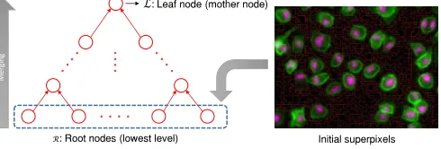
entails important extensions. The proposed hierarchical graph structure (Fig. 1) is made based on an initial superpixelation step [42], and subsequently merges the most similar superpix-els (graph nodes) until the highest level. The graph structure is asymmetric and irregular. This property allows capturing more natural cell boundaries for a more complex implementation.
Conversely, Laferteet al.use symmetric and regular quadtrees,
where the nodes are represented by square regions. The shapes of the nodes do not match the actual morphologies of the cells, rendering the method unsuitable for comparison. Inference-wise, our method uses features extracted by convolutional neural networks (CNN) (details explained in section IV-F) and is applied to supervised multi-class image segmentation, while
Laferteet al.use pre-defined intensity and texture features for
an EM-based unsupervised image classification. See Table I
for a summary of fine differences between the three mentioned
methods.
This paper significantly extends our preliminary work pre-sented in [43] through the following specific contributions:
• The role of features in the final segmentation performance
of intensity with an automatic feature selection scheme, employing the most relevant features for the analysis.
• We have shown how deep features from recent
convo-lutional neural networks can be systematically exploited within the proposed polytree framework for improved segmentation quantities.
• Polytrees are compared to customized trees, and
state-of-the-art CNNs, namely SegNet [44], DeepLab [45] and PSPNet [46], using synthetic and two real microscopy image datasets.
• A novel mechanism is employed to predict possible
errors in the segmented images, by comparing the label configurations with the imposed label constraints.
• The error introduced through the superpixel generation
step of the algorithm is analyzed for more accurate evaluation of the inference.
III. Method
Herewith, we present our proposed graphical model for image segmentation. First, a polytree is generated for the image, grouping similar pixels and regarding them as nodes in the graph. Next, the parameters of the likelihood functions are trained and labels of the nodes are inferred. Finally, the segmented image is constructed based on the optimal labels on the graph.
A. Graphical modeling for image segmentation
We perform the image segmentation by reformulating it as the problem of finding the optimal labeling for a graphical model, generated based on the image. The graph contains two types of nodes that represent the latent variables and the observations for their corresponding part of the image. Given the observations, finding the values of the latent variables is equivalent to labeling the corresponding area in the image i.e.
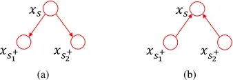
segmenting the image. As shown in Fig. 2a, each element s
(representing an area in the image) in the graph G with M
elements comprises a latent variable node xs attached to an
observation node ys. This label-observation configuration is an
element of the graph, in which ys and xs can be considered
as input and output values, respectively. The latent variable
xs ∈ X (X being the set of all latent variable nodes) takes
a discrete value from the label set Λand ys contains feature
vectors extracted from its corresponding area in the image. The process of generating the graph and labeling it based on the imposed priors is explained in the rest of this section.
B. Graph generation
Initially, the graph is generated grouping pixels into locally coherent areas (superpixels), each representing a single root node (Fig. 1). We use the SEEDS algorithm [42], which refines an initial grid of identically block shaped superpixels into more coherent ones. The two most similar superpixels are then recursively merged to generate higher-level nodes in the graph hierarchy, in a similar manner to generating a merge-tree [47]. For each superpixel at the finest level, one (root) node in the lowest level of the graph is created (see Fig. 1). Every two
: Leaf node (mother node)
: Root nodes (lowest level) Initial superpixels
M
e
rg
in
[image:4.612.319.564.59.142.2]g
Fig. 1. Generating a polytree from an oversegmented input image.
nodes achieving highest scores according to a similarity metric are then merged to create a new super node. The new super node is the union of image regions attached to its two lower level descendant nodes. We define the similarity metric as a superposition of distances using spatial and intensity features
of the superpixels. A vector β = [βs;βi] is introduced to
adjust contributions of each feature in the similarity metric. An
adaptive scheme is designed for settingβ, which helps in the
generation of more meaningful nodes on the graph. Nodes in lower levels of the graph represent subregions of objects, rather
than their full areas. For these nodes, we set β such that βs
consists of greater values compared toβi. This makes merging
neighboring nodes that correspond to parts of the same object (i.e. a cell or a nucleus in our case) more probable. In higher
levels, however, values ofβiare set to be greater than those of
βs to facilitate the merging of regions belonging to the same
class, although they might not be neighbors. Assumingβi=βi1
andβs=βs1 and settingβi=1 for simplicity, βis determined
by a cross validation merely onβs.
After each merging step, the new node and all the other
orphan nodes, are assessed with the similarity metric to recognize candidate nodes for merging next. Region merging is continued until only two orphan nodes remain in the graph, which are eventually merged to create the leaf node that corresponds to the whole image (Fig. 1). Since two nodes are merged at each step of the graph evolution, the resulting structure is a binary graph; i.e. each non-root node has two de-scendant nodes directly connected to it. We call this three-wise
structure acliqueand denote it by parent1−child−parent2.
Figure 2b shows a symbolic process of merging for a cell
(C) with a nucleus (N). Here, nodes 1 and 2 align with blue
and yellow areas in the synthetic cell. If these two nodes are chosen to be merged based on their value in the similarity metric, node 3 is generated, which corresponds to the union of blue and yellow areas annotated by the dashed ellipse. This
clique is represented by 1−3−2.
C. Graph definition
The generated graph is a hierarchical structure modeling the
interrelations between areas corresponding to different classes.
Nodes in lower levels correspond to smaller superpixels, such as sub-areas of cells, and are therefore more homogeneous. Higher level nodes correspond to one or multiple objects
that can be of different classes. The hierarchical structure
TABLE I
Summary of key differences betweenLaferteet al.method and the proposed tree and polytree
Method Laferteet al. Proposed tree Proposed polytree
Number of descendants 4 2 2
Hierarchical structure Regular Irregular Irregular
Features Intensity and texture CNN Intensity features/CNN
Application Unsupervised segmentation Supervised segmentation Supervised segmentation
Sample constructing element
�∀
� ∀#
∃ �
∀% ∃
�∀
� ∀#
∃ �
∀% ∃
(a)
1 2
3 3
1 2
[image:5.612.90.259.371.429.2](b)
Fig. 2. Explanation of the graphical model used for segmentation. A
label-observation elementscorresponding to an area in the image is shown in (a),
in which the blue plate representsMelements of which only an example is
shown. Panel (b) shows a symbolic process of node merging for a synthetic cell (C) with a nucleus (N) resulting a polytree constructing element.
�∀
� ∀#
∃ �
∀% ∃
(a)
�∀
� ∀#
∃ �
∀% ∃
(b)
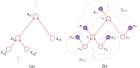
Fig. 3. Edge directions on cliques in directed tree (a) and polytree graphical
models (b).
different classes (in higher levels) according to certain merging
rules. These rules are introduced in the model by defining and applying priors on label configurations. In this setting,
segmenting the image equals inferring labels xs given the
observations ys∈Y(Ybeing the set of all observation nodes),
where the label configurations comply with the prior imposed on the model.
D. Imposing priors on the graph
Applying inclusion-based prior knowledge is the main ad-vantage of using hierarchical graphs and is a way to constrain the solution to plausible results. In a directed graphical model, prior knowledge can be modeled through setting specific forms of the conditional probabilities that implement causality according to the directions of the edges. These probabilities act as the prior factor in the Bayesian factorization of the posterior.
In directed trees, the joint probability consists of one-to-one priors that can only model across-level dependencies. For instance, in the constructing element of a dyadic tree depicted in Fig. 3a (excluding the observation nodes tem-porarily for simplicity) the joint probability is written as
p(X) = p(xs+
1|xs)p(xs
+
2|xs)p(xs), where p(xs
+
1|xs) and p(xs
+
2|xs)
are the one-to-one priors. In polytrees however, the joint probability has multiple-to-one priors modeling both across-level and same-across-level dependencies. The joint probability for
the sample polytree structure of Fig. 3b is factorized asp(X)=
p(xs|xs+
1,xs
+
2)p(xs
+
1)p(xs
+
2), in which the factor p(xs|xs
+
1,xs
+
2) is
the prior. To show how this can influence the modeling ability of the hierarchy, imagine the label set consists of two classes:
Λ ={A,B}. Also, assumeB−A−Ais a feasible andB−A−Bis
an unfeasible configuration. Using trees,B−A−Ais allowed by
setting probabilities p(xs+
i =B|xs=A) and p(xs
+
i =A|xs =A)
to non-zero values. However, enforcing the former constraint
also makesB−A−Bcliques feasible, even though they are to
be prevented by the model. But thanks to the more complex
priors in the polytree, setting p(xs = A|xs+
1 = B,xs
+
2 = A) to
non-zero values and setting p(xs=A|xs+
1 =B,xs
+
2 =B) to zero
satisfies both of the constraints with no conflicts. This simple example shows the advantage of polytrees over directed trees in modeling more complex problems, by using a larger number of parameters.
In this paper, we use the generated polytree (details ex-plained in section III-B) to segment the image by inferring the optimal labels for latent variable nodes. Each node at the lowest graph level (finest image resolution) is a root (in contrast to the single root node in directed trees) and there is only one leaf node (see Fig. 1).
Figure 4 shows the tables of priors p(xs+
1|xs) in trees and
p(xs|xs+
1,xs
+
2) in polytrees, and possible label configurations,
when three classes of background (B), cell (C) and nucleus (N)
exist in the image. Conditional probabilities were set to zero
for implausible configurations, e.g. p(xs =C|xs+
1 = B,xs
+
2 =
B)=0, and to nonzero for plausible configurations, e.g.p(xs=
B|xs+
1 =B,xs
+
2 =B)=1. For cases where no child label xs is
possible for a pair of parent labelsxs+
1 andxs
+
2, a uniform prior
was considered, e.g. p(xs|xs+
1 =B,xs
+
2 =N)=1/3.
E. Label inference
Let X = {xs} and Y = {y
s} denote sets of labels (latent
variables) and the corresponding observed features at nodes,
respectively,G denote the set of nodes and edges and xs∈Λ,
whereΛis the set of all possible labels. For an internal node
(neither in the lowest level nor the leaf node) sin the graph,
s−, s+and s′ denote nodes in higher, lower and same layers,
(a) (b)
Fig. 4. The prior knowledge used in this paper for the three-class problem of cell and nucleus segmentation. Panel (a) shows the plausible label-configurations based on the inclusion of nuclei by cells and cells by the background. Panel (b) shows equivalent probabilistic conditionals when directed trees or polytrees
are used for modeling the image. When no child labelxsis plausible for a pair of parent labelsxs+
1 andxs
+
2, a uniform prior 1/3 was considered.
We now derive equations governing the posterior
probabili-ties of graph nodes. Given the observed dataY, finding the best
segmentation equals the best configuration of labelsXfor the
graph. Bayesian inference associates the most probable label
from the set of possible labels Λ, given all observations:
∀s∈G,xˆs=arg max
xs∈Λ
p(xs|Y) (1)
A new set of equations is derived to calculate the closed-form posterior probabilities at each node in the polytree. The inference algorithm calculates the posteriors of the nodes in two passes. These two consist of a pass from the leaf to the
roots, (top-down pass), and another from the roots to the leaf
(bottom-up pass).
The probability of a node’s label xs, given all data Y, is
computed by marginalizing the probability of the clique over
two parent nodes s+1 and s+2 givenY, and the joint posterior
is given by
p(xs|Y)= X
xs+
1,xs
+
2
p(xs,xs+
1,xs
+
2|
Y)
(2)
Three-wise constraints on cliques appear in the posterior calcu-lation. To factorize the joint probability, we need a mechanism to identify the dependency of the nodes in the graph.
D-separation: Consider three sets of nodesA, B andC in a directed acyclic graph. We want to verify the conditional
dependency of A and B, given C. D-separation (directional
�∀ �∀#
�
∀∃
% �
∀&%
�∀∋
[image:6.612.70.543.65.179.2](a) (b)
Fig. 5. Distribution of latent and observation nodes on the graph. The notation
for nodes connected to an internal node sof the graph is shown in (a). In
(b), the graphical representation of ascendant,Ya(s), and descendant,Yd(s),
observation nodes is depicted.
separation) rule [31] can determine this based on the paths
that exist betweenAandBon the graph. Each path connecting
A and B is blocked if it involves a node sfor which either:
a) arrows meet head-to-tail or tail-to-tail at node s and s ∈
C (Fig. 6a), or b) arrows meet head-to-head at node s and
neither the node nor any of its descendants are in the set C
(section 6b). If all paths from A andB are blocked, they are
conditionally independent, givenC (Aand B are d-separated
byC andAyB|C).
[image:6.612.325.555.369.423.2](a) (b)
Fig. 6. D-separation rule. Nodes Aand Bare conditionally independent
givenC, when graph edges meet head-to-tail or tail-to-tail ands∈C(a), or
when graph edges meet head-to-head ands<C(b).
Using the d-separation rule, the joint posterior in Eq. 2 is expanded as
p(xs,xs+
1,xs
+
2|
Y)=p(xs|xs+
1,xs
+
2,
Y)p(xs+
1,xs
+
2|
Y)
=p(xs|xs+
1,xs
+
2,Ya(s))
p(xs+
1,xs
+
2|Ya(s
+
1,s
+
2),Yd(s
+
1,s
+
2)),
(3)
where Ya(.) and Yd(.) refer to the sets of observation nodes
of the ascendant and descendant nodes, respectively (Fig. 5b).
For each nodes(or a set of nodesS), ascendant nodes refer to
the set of all nodes that are connected to s(S) through edges
with inward directions. Similarly, descendant nodes include the
nodes connected to nodes(S) through outward oriented graph
edges. The union of ascendant and descendant observation nodes constructs the set of all observations. See Fig. 5b for a graphical explanation.
We first elaborate on the factor p(xs|xs+
1,xs
+
2,Ya(s)) on the
right-hand side of Eq. 3. This factor enforces posteriors of unfeasible configurations to zero, as it is a product of the joint probability of a child node and its two parent nodes.
p(xs|xs+
1,xs
+
2,Ya(s))=
p(xs,xs+
1,xs
+
2|Ya(s))
P x′
sp(x
′
s,xs+
1,xs
+
2|Ya(s))
[image:6.612.52.292.587.704.2]Using the d-separation rule, the numerator becomes:
p(xs,xs+
1,xs
+
2|Ya(s))=p(xs
+
1,xs
+
2|xs)p(xs|Ya(s))
= p(xs,xs
+
1,xs
+
2)
p(xs)
p(xs|Ya(s)).
(5)
The factor p(xs,xs+
1,xs
+
2) in Eq. 5 controls the occurrence of
feasible and unfeasible configurations on the graph, by setting
nonzero and zero values, respectively. The factor p(xs|Ya(s)) in
Eq. 5 is the posterior of node s given the observations of all
its ascendant nodes and its own observations. This top-down
posterior is expanded as:
p(xs|Ya(s))∝ X
xs−,xs′
p(ys|xs)p(ys′|xs′)p(xs′|Yd(s′))
p(xs,xs′,xs−)
p(xs−)p(xs′)
p(xs−|Ya(s−)).
(6)
Equation 6 indicates that having calculated the likelihood probabilities p(ys|xs), p(ys′|xs′), and the posterior p(xs′|Yd(s′)),
the top-down posterior of node s is calculated based on
top-down posterior of the node s−. This implies that a top-down
recursion calculates the top-down posteriors for all nodes.
The factorp(xs+
1,xs
+
2|Ya(s
+
1,s
+
2),Yd(s
+
1,s
+
2)) on the right-hand side
of Eq. 3 is factorized by several applications of d-separation rule. This factorization separates parts calculated from ascen-dant and descenascen-dant nodes as follows.
p(xs+
1,xs
+
2|Ya(s
+
1,s
+
2),Yd(s
+
1,s
+
2))
∝p(Ya(s+
1,s
+
2),Yd(s
+
1,s
+
2)|xs
+
1,xs
+
2)p(xs
+
1,xs
+
2)
=p(Ya(s+
1,s
+
2)|xs
+
1,xs
+
2)p(Yd(s
+
1,s
+
2)|xs
+
1,xs
+
2)p(xs
+
1,xs
+
2)
=p(Ya(s+
1,s
+
2)|xs
+
1,xs
+
2)p(Yd(s
+
1)|xs
+
1)p(Yd(s
+
2)|xs
+
2)p(xs
+
1,xs
+
2)
∝p(xs+
1,xs
+
2|Ya(s
+
1,s
+
2))
p(xs+
1|Yd(s
+
1))
p(xs+
1)
p(xs+
2|Yd(s
+
2))
p(xs+
2)
(7)
Similar to Eq. 6, p(xs+
1,xs
+
2|Ya(s
+
1,s
+
2)) on the right-hand side
of Eq. 7 is calculated through a top-down recursion as below.
p(xs+
1,xs
+
2|Ya(s
+
1,s
+
2))∝
X
xs
p(ys+
1|xs
+
1)p(ys+2|xs
+
2)
p(xs+
1,xs
+
2|xs)p(xs|Ya(s))
(8)
The factors p(xs+
1|Yd(s
+
1)) andp(xs
+
2|Yd(s
+
2)) in Eq. 7 are called
bottom-up posteriorsas they are calculated based on posteriors
of their descendant nodes. For each node sin the graph, the
bottom-up posterior is written as
p(xs|Yd(s))∝ X
xs+
1,xs+2
p(ys+
1|xs
+
1)p(ys+2|xs
+
2)
p(xs+
1|Yd(s
+
1))p(xs
+
2|Yd(s
+
2))p(xs|xs
+
1,xs
+
2).
(9)
Derivations of Eq. 6, 8 and 9 are included in Appendix A. Making use of Eq. 3, 4, 5 and 7, the node’s posterior in Eq. 2, given all the observations, is written as follows.
p(xs|Y)∝ X
xs+
1,xs
+
2
p(xs,xs+
1,xs
+
2|Ya(s))
P x′
sp(x
′
s,xs+
1,xs
+
2|Ya(s))
p(xs+
1,xs
+
2|Ya(s
+
1,s
+
2))
p(xs+
1|Yd(s
+
1))
p(xs+
1)
p(xs+
2|Yd(s
+
2))
p(xs+
2)
(10)
Equation 10 calculates the posterior at each node
s using three marginal posteriors p(xs,xs+
1,xs
+
2|Ya(s)),
p(xs+
1,xs
+
2|Ya(s
+
1,s
+
2)) and p(xs|Yd(s)), in Eq. 5, 8 and 9. Each
term is calculated through either a top-down or a bottom-up recursion. The inference is summarized in Algorithm 1. Note
that R andL denote the set of root nodes and the leaf node
in the graph, respectively.
Algorithm 1 Label inference on polytrees
Preliminary pass. This initial upward recursion computes
prior marginals for each node. The parameters p(xs|xs+
1,xs
+
2)
are set based on problem the model represents, as explained in Fig. 4 and section III-D.
for all s∈Rdo
p(xs)= |Λ1|
end for
for all s<Rdo
p(xs)=Pxs+
1,xs
+
2
p(xs|xs+
1,xs
+
2)p(xs
+
1)p(xs
+
2)
p(xs+
1,xs
+
2|xs)=
p(xs|xs+
1,xs+2)p(xs+1)p(xs+2)
p(xs) end for
△ Bottom-up pass. Upward recursion for calculating
bottom-up posteriors of nodes.
for all s∈Rdo
p(xs|Yd(s))=p(xs)
end for
for all s<Rdo
p(xs|Yd(s))∝Pxs+
1,xs
+
2
p(ys+
1|xs
+
1)p(ys+2|xs
+
2)
p(xs+
1|Yd(s
+
1))p(xs
+
2|Yd(s
+
2))p(xs|xs
+
1,xs
+
2)
end for
∇Top-down pass. Downward recursion for calculating
top-down posteriors and calculation of complete posteriors from marginal posteriors.
if s=L then
p(xs|Ya(s))=p(xs|ys)∝p(ys|xs)p(xs)
end if
for all s,Ldo
p(xs|Ya(s))∝Pxs−,xs′p(ys|xs)p(ys′|xs′)p(xs′|Yd(s′))
p(xs,xs′|xs−)
p(xs′) p(xs−|Ya(s−))
p(xs,xs+
1,xs
+
2|Ya(s))=p(xs
+
1,xs
+
2|xs)p(xs|Ya(s))
p(xs+
1,xs
+
2|Ya(s
+
1,s
+
2))
∝P
xsp(ys+1|xs+1)p(ys+2|xs
+
2)p(xs
+
1,xs
+
2|xs)p(xs|Ya(s))
end for
IV. Experiments and results
A. General experimental design
of edges and therefore the use of two-wise priors instead of
three-wise priors affect the results. For inferring posteriors on
trees, we adapted Laferteet al.[33] formulation into the graphs
generated in this work.
B. Validation of the inference algorithm: ancestral sampling
To assess the performance of the inference algorithm, re-gardless of the image processing tools employed, we com-pared polytrees to trees on the classification of synthetic data generated by ancestral sampling technique. Samples are drawn
for xs variables to represent ground truth data. Based on this,
the ys variables are then drawn according to the presumed
class conditional distributions. Next, ignoring the reference xs
variables of the first step, new values are inferred for xs from
the observed ys variables only. We then compare the inferred
xs variables to the ground truth and experimentally validate
the viability of our inference algorithm.
To draw samples ˆx1,xˆ2, ...,xˆN from the joint distribution
p(X,Y), we first sample from the probability distribution
p(xs)
s∈R for all root nodes. Visiting each internal node in an
upward recursion, we sample from the conditional distribution
p(xs|xs+
1,xs
+
2), where the parent labels ˆxs
+
1 and ˆxs
+
2 have been
sampled in previous steps. Once we have sampled from the
leaf node of the graph, ˆxN, we will have obtained a sample
from the joint distribution p(X,Y).
In this section only, we considered two classes for xs for
simplicity, and selectedysfrom the continuous range of [0,1].
Class conditional likelihood functions, p(ys|xs) were Beta
distributions. For different numbers of root nodes ranging from
10 to 100000 (i.e. 19 to 199999 nodes in total as the graph is binary), graphs with random structures were generated and labels were inferred. Figures 7a and 7b show Beta
distribu-tions for different selectivities. Figures 7c and 7d depict the
percentages of the wrongly inferred labels for different graph
sizes and the corresponding Beta distributions in directed trees and polytrees, respectively. Results show that polytrees achieve higher accuracies in predicting labels of graph nodes, com-pared to directed trees. This experiment shows that even with significant overlaps between the likelihoods of two classes,
wherea>0.8, the polytree inference error is stable and small
(i.e., less than 10%). Therefore, this experiment verifies the correctness of the developed derivations and also indicates that inference accuracy increases with the selectivity of the likelihood functions.
C. Oversegmentation performance evaluation
The SEEDS oversegmentation algorithm [42], used for gen-erating superpixels, finds areas in the image based on intensity homogeneity and boundary smoothness. Ideally, all of the object and within-object boundaries should lie on superpixel boundaries. However, due to the existence of noise and illumi-nation artifacts in the images, not all the superpixels accurately resemble boundaries. To investigate the error introduced by oversegmentation, we labeled the superpixels in the image merely according to the ground truth, to calculate the max-imum achievable segmentation accuracy for the segmentation algorithms employing SEEDS. To do this, the label of each
superpixel was set based on the labels of the majority of its pixels in the Ground Truth. Figure 8 shows two samples from BBBC020 and BBBC007 datasets, for which the overseg-mented image and the labeled superpixels can be compared
to the ground truth. The Dice similarity coefficients (DSC)
between the labeled superpixels and the ground truth in Fig. 9 quantitatively show the maximum segmentation accuracy that the graph-based algorithms employing superpixels in this work can achieve for the two datasets.
D. Validation on multi-class image segmentation
The proposed algorithm was applied to the problem of supervised multi-class image segmentation, and to evaluate the role of exploiting prior knowledge in segmentation. Two real image datasets were chosen from the publicly avail-able datasets on Broad Bioimage Benchmark Collection that contain two-channel fluorescence microscopy images with cells and nuclei, namely BBBC020 and BBBC007 datasets [48]. In these cases, between-class relationships can help to improve the segmentation results, as only a certain set of label configurations are plausible. The results of this experiment were compared to those of SegNet, DeepLab and PSPNet.
BBBC020 contains 20 two-channel in vitro microscopy
images of murine bone marrow macrophages, and BBBC007
has 16 two-channelin vitro microscopy images of drosophila
Kc167 cells. Manual annotations are available for both datasets. These two datasets have the same type of images and define similar multi-class segmentation problems of cells and nuclei. The BBBC007 dataset has a larger number of overlapping cells and noisier images, which makes the seg-mentation more challenging. See Fig. 10 for samples from the two datasets.
To explore the role of features used for inference, we used two types of features: 1) scale-space first and second order
differential invariants [49], 2) deep representations extracted
by SegNet. In the following, details of experiments with the two feature sets are explained and results are compared to the three convolutional neural networks. The accuracy of the segmentation was measured by calculating confusion
matrices and the Dice similarity coefficients [50] computed
by comparing the segmentation results with the ground truth.
E. Polytree with scale-space differential invariant features
In this experiment, features were chosen to be intensity value, the absolute value of the gradient, and determinants and traces of Hessian matrix at 7 scales, for each microscopy channel. A total of 32 features were initially calculated for each image, out of which the most relevant features were selected using Fisher discriminant score [29]. Fisher scores,
Wd, are weights with higher values for features that have
higher discrimination abilities and are calculated as follows.
Wd= PK
c=1(md−md,c)2 PK
c=1s2d,c
K
K−1 (11)
Wheredis the index of the feature,Kis the total number of
0 0.5 1 y
0 2 4 6 8 10
(y|b,a)
a = 0.2 a = 0.4 a = 0.6 a = 0.8 a = 1
(a)
0 0.5 1
y 0
2 4 6 8 10
(y|a,b)
a = 0.2 a = 0.4 a = 0.6 a = 0.8 a = 1
(b)
10 100 1000 10000 100000
Number of root nodes R 0
5 10 15 20
Error (%) for tree
(c)
10 100 1000 10000 100000 Number of root nodes R 0
5 10 15 20
Error (%) for polytree
[image:9.612.51.556.64.167.2](d)
Fig. 7. Panels (a) and (b) show Beta distributions used as class conditional likelihood functions in ancestral sampling. The value ofbwas fixed and curves
correspond to the values ofaranging from 0.2 to 1, respectively, with an increasing overlap on the likelihoods (thus potential classification errors). In (c) and
(d), the percentages of wrongly inferred labels using ancestral sampling are shown for tree and polytree models, respectively.
[image:9.612.74.536.214.399.2]Input image Oversegmented image Labeled oversegmentation Ground truth
Fig. 8. Evaluating the performance of the oversegmentation. First and second rows show the superpixels and the best possible labeling of the image using
the generated superpixels, for two samples from BBBC020 and BBBC007 datasets, respectively. The finest superpixels were not shown in the oversegmented images for a better visualization.
(a) (b)
Fig. 9. Dice similarity coefficients between the labeled superpixels and the
ground truth on (a) BBBC020 and (b) BBBC007 datasets. These values show the accuracy of the SEEDS oversegmentation algorithm [42] in generating superpixels.
md,candsd,cdenote mean and standard deviation ofdth feature
within samples of cth class, respectively.
For each dataset, four images were used for feature selection through ranking features based on their Fisher scores. The rest of the images were used for cross validation, i.e. 4- and 6-fold
cross validations were applied on the 16 and 12 remaining images in BBBC020 and BBBC007 datasets, respectively. The four images used for Fisher score calculation were always included in the training sets during cross validation.
Once the Fisher scores were calculated, features were
ranked for each class separately, and the firstF of them were
selected for classification. Gaussian distributions were used for class conditional likelihood functions with a layer dependent variance that allows higher within-class variances for nodes in the higher levels of the graph. Parameters of the method,
including βs (explained in section III-B), number of intensity
features used for graph generation (D) and inference (F), and
values of mean (µc) and covariance matrix (Σc) for each class
care optimized through cross validation for each of the two
datasets. Figure 11 shows the block diagram of polytree and
tree based segmentation using scale-space differential invariant
features.
We applied SegNet to the two datasets and compared the results with polytree and tree segmentation using scale-space
differential invariants. As the size of the datasets was not suffi
[image:9.612.50.303.461.624.2]Input image Ground truth Tree+SS Polytree+SS SegNet DeepLab PSPNet Tree +SN Polytree+SN
Fig. 10. Sample images from BBBC020 (first and second rows) and BBBC007 (third and fourth rows), their corresponding ground truth and automatic segmentations. Third and fourth columns show segmentation results using trees and polytrees with scale-space (SS) features (section IV-E), respectively. Fifth, sixth and seventh columns show results of applying SegNet, DeepLab and PSPNet to the images, respectively. The last two columns depict segmentation
results using directed trees and polytrees with features generated by SegNet, labeled Tree+SN and Polytree+SN, respectively.
Test Set
Oversegmentation
Graph generation Label inference Segmented Images
Learning node labels
Learning likelihood parameters
Scale-space differential invariants
for each channel SEEDS
Training Set
K-fold cross validation
Validation set
Training set
Feature extraction
[image:10.612.53.561.55.239.2]Fisher ranking
Fig. 11. Block diagram for polytree and tree segmentation with scale-space differential invariant features.
two datasets was increased to 400 images (chosen based on
experiments with different numbers of augmented images) to
improve shift and rotation invariance, and robustness to de-formations and gray value variations [51], [52]. Furthermore, 5000 iterations were performed for the experiments on the two datasets with the cost function reaching its minimum after about 1000 iterations. The trained network was then evaluated on its segmentation of the test set. Figure 12 shows the con-fusion matrices for SegNet, tree and polytree segmentations of BBBC020 and BBB007 datasets. The overall segmentation accuracies are similar for the three methods on BBBC020 dataset, while SegNet outperforms the other two on BBBC007.
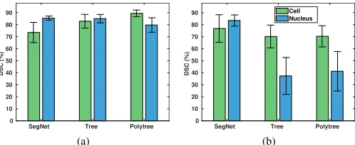
Dice similarity coefficients (DSC) in Fig. 13 indicate SegNet
is more accurate than tree and polytree in both classes on the BBBC007, while tree and polytree provide higher DSC values for the segmentation of cells in BBBC020. DSC values for the
segmentation of nuclei in BBBC020 are similar for SegNet and tree, being more accurate than that for polytree.
This experiment indicates outperformance of SegNet in segmentation. However, the three methods were compared
using different experimental setups. First, SegNet was trained
using a larger set of training images (through augmentation).
The numbers of features (F) selected after ranking them
based on the Fisher scores were 20 and 6, for BBBC020 and BBBC007 datasets, respectively, which are very small compared to the number of features extracted by SegNet. To investigate the methods regardless of the type of features used, we propose the use of polytrees with features employed by SegNet in the next section.
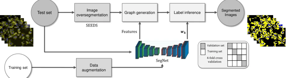
F. Polytree with SegNet-based deep features
[image:10.612.52.554.295.504.2]background cell nucleus Target Class background cell nucleus Output Class 1748996 50.6% 382156 11.1% 27320 0.8% 81.0% 19.0% 189865 5.5% 847360 24.5% 30928 0.9% 79.3% 20.7% 3271 0.1% 31546 0.9% 194558 5.6% 84.8% 15.2% 90.1% 9.9% 67.2% 32.8% 77.0% 23.0% 80.8% 19.2% (a)
background cell nucleus Target Class background cell nucleus Output Class 13913421 60.2% 2427332 10.5% 376222 1.6% 83.2% 16.8% 1198933 5.2% 3840586 16.6% 223008 1.0% 73.0% 27.0% 98 0.0% 133420 0.6% 983300 4.3% 88.0% 12.0% 92.1% 7.9% 60.0% 40.0% 62.1% 37.9% 81.1% 18.9% (b)
background cell nucleus Target Class background cell nucleus Output Class 13962506 60.5% 2488609 10.8% 265860 1.2% 83.5% 16.5% 1247208 5.4% 3880283 16.8% 135036 0.6% 73.7% 26.3% 114 0.0% 260664 1.1% 856040 3.7% 76.6% 23.4% 91.8% 8.2% 58.5% 41.5% 68.1% 31.9% 81.0% 19.0% (c)
background cell nucleus Target Class background cell nucleus Output Class 1439207 52.1% 124223 4.5% 11458 0.4% 91.4% 8.6% 138962 5.0% 574425 20.8% 77362 2.8% 72.6% 27.4% 10200 0.4% 69848 2.5% 319115 11.5% 79.9% 20.1% 90.6% 9.4% 74.7% 25.3% 78.2% 21.8% 84.4% 15.6% (d)
background cell nucleus Target Class background cell nucleus Output Class 1380139 53.9% 333212 13.0% 2579 0.1% 80.4% 19.6% 43296 1.7% 500801 19.6% 5549 0.2% 91.1% 8.9% 3377 0.1% 216400 8.5% 74647 2.9% 25.4% 74.6% 96.7% 3.3% 47.7% 52.3% 90.2% 9.8% 76.4% 23.6% (e)
background cell nucleus Target Class background cell nucleus Output Class 1404567 54.9% 306553 12.0% 4810 0.2% 81.9% 18.1% 46510 1.8% 495851 19.4% 7285 0.3% 90.2% 9.8% 4050 0.2% 209676 8.2% 80698 3.2% 27.4% 72.6% 96.5% 3.5% 49.0% 51.0% 87.0% 13.0% 77.4% 22.6% (f)
Fig. 12. Confusion matrices for SegNet with augmented images, tree and
polytree segmentations with scale-space differential invariants on the two real datasets. The overall accuracies of tree (b) and polytree (c) were slightly higher than SegNet (a) on the BBBC020 dataset, while SegNet (d) outperforms tree (e) and polytree (f) on the BBBC007 dataset. Number of pixels corresponding to each percentage is shown in bold. Black and white percentages in each box show the proportion of correctly and incorrectly classified pixels, respectively.
and training size, we developed a framework to employ fea-tures calculated by SegNet, shown in Fig. 14. In this section, we have also applied directed trees with SegNet features to the segmentation of images in the two datasets. The directed tree was generated by reversing the directions of edges on the
irregular polytree and the inference proposed by Laferte et
al. was adapted to it. Softmax [29] functions were chosen as
posteriors.
p(xs=c|ys)∝
exp(wT
cys) PK
k exp(w T kys)
(12)
In Eq. 12, wk’s are the vectors of weights for each class
k, calculated by the CNN to describe the distribution of each
class, andKdenotes the total number of classes (K=3 in our
case).
SegNet Tree Polytree 0 10 20 30 40 50 60 70 80 90 DSC (%) (a)
[image:11.612.314.563.64.166.2]SegNet Tree Polytree 0 10 20 30 40 50 60 70 80 90 DSC (%) Cell Nucleus (b)
Fig. 13. Dice similarity coefficients (DSC) of polytree and tree based
segmentations using scale-space differential invariant features compared to
SegNet on (a) BBBC020 and (b) BBBC007 datasets.
Note that Eq. 12 implies that a set of improper (unnormal-ized) class conditional likelihoods, i.e. exponentials, have been used. However, looking at Algorithm 1, the proposed inference algorithm normalizes every term that contains likelihood prob-ability of nodes, facilitating the utilization of unnormalized likelihood functions. For this reason, we chose exponentials
as the likelihood functions, i.e. p(ys|xs = c) ∝ exp(wTcys).
Both of the class parameters (wc) and feature vectors (ys) are
provided by the SegNet. Therefore, having trained the SegNet, we do not require any additional training steps.
In this section, we compared the results of the proposed polytree and tree methods with SegNet, Deeplab and PSPNet. In applying the CNNs on BBBC020 and BBBC007 datasets, the same image augmentation procedure as explained in sec-tion IV-E was employed. Segmentasec-tion performance of the
methods were compared at three different sizes of datasets;
original dataset size (20 images for BBBC020 and 16 images for BBBC007), 200, and 400 augmented images. In each of the experiments, a four-fold cross validation was done. To perform a cross validation, the augmented images were generated based only on the images in the training folds, so that the network was trained independently of the testing set.
For these experiments, the images were first oversegmented using the SEEDS algorithm [42]. The features provided by SegNet were then used for graph generation and, in the next
[image:11.612.54.289.73.476.2]step, for label inference (F=D).
Figure 15 shows the DSC of the five methods when SegNet features are used for polytree and tree with variable numbers of the training samples. Table II shows average accuracy values for each of the five methods and for each size of the training set for BBBC020 and BBBC007 datasets. The superior results of
the directed tree and polytree indicate the effectiveness of the
prior knowledge imposed by these directed graphical models, which cannot be explicitly modeled by CNNs. It can also be seen that the performance of directed trees tend to have larger variances compared to polytrees. This higher uncertainty is likely to stem from the inability of directed trees to eliminate unfeasible label configurations, eliminated by polytrees, that allows semantically wrong segmentations (see section III-D). To assess the complexity of the segmentation algorithm, graph generation and Bayesian inference stages were timed for graphs ranging from 20 to 200000 nodes. Results show
that the time of run, t, on a machine equipped with Intel
Test set Image
oversegmentation Graph generation Label inference
Segmented Images
SEEDS
Features
SegNet 4-fold cross validation
Validation set
Training set
Training set Data
[image:12.612.73.548.59.188.2]augmentation
Fig. 14. The proposed architecture for using SegNet-based deep features and learning class conditional likelihood functions.
[image:12.612.50.567.234.434.2](a) (b)
Fig. 15. Dice similarity coefficients of the five methods for segmenting cells and nuclei in (a) BBBC020 and (b) BBBC007 datasets, respectively.
TABLE II
MeanDice score coefficients of the five methods onBBBC020andBBBC007datasets.
Dataset BBBC020 BBBC007
# Images 20 200 400 16 200 400
Polytree 78.60±5.42 80.43±4.76 81.35±5.18 80.28±8.44 82.09±7.46 83.06±6.85
Directed tree 78.45±5.39 80.52±4.82 81.45±5.21 79.65±10.62 81.00±10.40 81.75±9.64
SegNet 77.00±5.28 79.42±4.71 80.40±5.06 77.40±8.83 80.06±7.79 81.03±7.43
DeepLab 78.17±3.73 81.35±2.60 81.37±2.98 79.96±5.97 80.56±5.95 80.75±4.95
PSPNet 76.72±3.14 78.35±3.30 78.27±3.13 78.37±4.84 77.56±4.50 77.37±4.71
Ubuntu 14.04, scales with the number of graph nodes,n, with
t=5×10⁻⁵n1.3 andt=2.4×10⁻⁶n2for graph generation and
inference, respectively. This shows a sustainable scalability of the proposed algorithm with increasing the number of nodes.
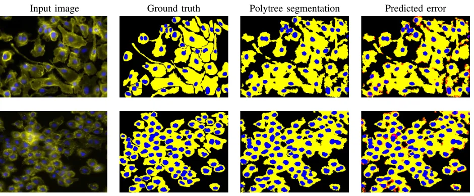
G. Prediction of segmentation error
Unlike discriminative models, generative models incorpo-rate priors in calculating the posterior distributions. Accord-ingly, the proposed polytree graphical model can evaluate to what extent its estimated clique labels comply with the im-posed priors. A strong disagreement can indicate an erroneous segmentation that can be flagged up for manual inspection. To implement this, the labels of cliques are read from the graph
representing the segmented image, and their probabilities are calculated using the constraints in Fig. 4b. Areas in the image that correspond to cliques with unfeasible labels (zero probabilities) are then marked as potential segmentation errors. Figure 16 shows samples from BBBC020 and BBBC007 and the error predicted for them. To represent the confidence of the model in labeling the wrongly segmented areas, they are
marked by red colors with different values, corresponding to
the entropy of the joint posterior of the clique. Areas with lower and higher error likelihoods (entropies), are shown in lighter and darker colors, respectively.
The error prediction ability of the directed trees was also
be-Input image Ground truth Polytree segmentation Predicted error
Fig. 16. The ability of the proposed method in nominating the possibly wrongly segmented areas shown for samples from BBBC020 (first row) and BBBC007 (second row) datasets. Value of red color is proportional to the probability of being an error in the segmentation.
(a) (b)
Fig. 17. Dice similarity coefficients between the predicted and the actual
segmentation error for directed trees and polytrees on (a) BBBC020 and (b) BBBC007 datasets.
tween the potentially incorrectly segmented areas and the actual segmentation error for both methods. Figure 18 shows
the average Dice similarity coefficients for different thresholds
of entropies for the models on the two datasets. These two figures indicate that polytrees are superior in predicting the segmentation error. This superiority is due to the more ef-fective imposition of prior knowledge in polytrees compared to trees (three-wise constraints versus two-wise constraints, respectively).
V. Discussion and conclusions
This work proposes a new inference algorithm for multi-class segmentation using irregular directed graphical models. The image is first oversegmented and a graph is generated by recursively merging the two most similar nodes in the graph until a hierarchical graphical model is generated that has no loops. Two types of features were used in this study: 1)
scale-space differential invariants of intensity and 2)
SegNet-based deep image representations. This was done to investigate
0 0.2 0.4 0.6 0.8 1 Entropy
0 5 10 15 20 25 30
Average DSC (%)
Tree Polytree
(a)
0 0.2 0.4 0.6 0.8 1 Entropy
0 5 10 15 20 25 30 35
Average DSC (%)
Tree Polytree
[image:13.612.72.542.53.248.2](b)
Fig. 18. Average Dice similarity coefficients between the predicted and actual segmentation error for directed trees and polytrees at different thresholds of entropies of cliques on (a) BBBC020 and (b) BBBC007 datasets.
the dependency of the method performance on the features used. Two publicly available real microscopy image datasets were used for evaluation. We showed that our polytree based method outperforms the customized tree and three state-of-the-art convolutional neural networks, SegNet [44], DeepLab [45] and PSPNet [46]. The oversegmentation performance was evaluated by comparing the labeled superpixels to GT to determine the maximum achievable accuracy of the segmen-tation methods employing the generated superpixels using the SEEDS algorithm [42]. In terms of predicting segmentation errors, polytrees also outperformed directed trees.
In the literature, directed graphical models have been em-ployed to incorporate prior knowledge to improve segmen-tation [23], [24]. However, a large majority of the works rely on directed trees, due to more simple inference and the
existence of efficient closed form solutions for posteriors. This
[image:13.612.56.566.300.463.2]polytree. The distinct orientation of edges on polytrees allows them to model label configurations for nodes in horizontal vicinity, in addition to the vertical nodes modeled by trees. This improves the compliance of the inferred labels with the imposed constraints and is a key feature of polytree, as modeling the same relations with Markov Random Fields requires graphs with loops, for which the inference is iterative and approximate. It should be noted that factor graphs [53] can also provide closed form solutions as long as the original graph structure can be converted to a factor graph without loops. However, the proposed inference method does not require the extra step for generating a second factor graph, simplifying the implementation.
Using polytrees with scale-space differential invariant
fea-tures (Fig. 13) suggests that depending on the choice of model features and parameters, it can outperform SegNet, even though the latter is trained on a much larger training set (16 vs. 400 images). Additionally, the distinct performance of the
polytree segmentation on BBBC007 dataset when different
types of features were used reveals the key role of features in the segmentation performance. By using the same features of the SegNet, polytree provides a superior segmentation compared to directed trees and three CNNs (see Table II). This superiority owes to the model’s ability to explicitly enforce prior knowledge and to eliminate unfeasible label configura-tions. An example of these configurations for the problem of segmenting cells and nuclei is the existence of a cell area inside a nucleus. CNNs can also learn such dependencies through their cascade of convolutional layers. However, their
efficiency relies on the quality of the training data and the
existence of sufficient instances of the dependencies, which
might not be possible for every dataset.
Evaluating the performance of oversegmentation shows that this stage significantly contributes to the overall segmentation error. The maximum achievable accuracies depicted in Fig. 9 show an upper bound for the Dice scores that could be achieved by segmentation methods employing SEEDS on the two datasets. Using other superpixel generation algorithms might address this problem by drawing superpixels with boundaries more accurately matching objects boundaries in the image.
[image:14.612.316.567.417.767.2]In the current implementation of the proposed algorithm, the overall segmentation performance of the method can be confined by the graph generation quality. To address this, one line of future work can be the development of a Maximum Posterior (MAP) estimation [29] for graph generation that optimizes the graph structure jointly with label inference. On the other hand, it is worth mentioning that the small margin of improvement by the proposed graph based segmentation over SegNet is because features learned by the CNN are minimizing the cost function of SegNet rather than the cost function of the polytree. Another line of future work can be extracting features by neural networks that are specifically minimizing the cost of polytree. In predicting the segmentation error, however, polytrees significantly outperform trees (see Fig. 17 and 18). The lower variance of the average DSC in Table II when using DeepLab and PSPNet is due to the additional network layers that that improve the localization
of boundaries for a cost of adding to the computational complexity. An extension of current work can be employing deep representations extracted by these two networks with the use of polytrees for incorporating prior knowledge for possible improvements in the segmentation results.
The proposed application of the directed graphical models facilitates extracting statistics of relationships between class la-bels from the graph, in addition to the current use of the graph for imposing prior knowledge. For example, using the pro-posed method for the segmentation of host and pathogen cells, the proportions of intracellular and extracellular pathogen cells, infected and healthy host cells can be calculated from the labeled graph, both at a specific time point and over time for disease progression monitoring. Such applications introduce new capabilities of graph based segmentation for the behavioral analysis of diseases and biological systems. Other than their use in the image analysis, polytrees can
model phenomena involving the interrelations of different
objects with underlying dependencies. One example can be the genetic networks where polytrees can model relationships
between different entities including genes or individuals and
the expression of certain genes in different generations. The
inference platform presented here can be extended to the case where each node can have more than two and generally an arbitrary number of descendant nodes to improve its adaptation to the problem being modeled.
AppendixA
Proofs of equations
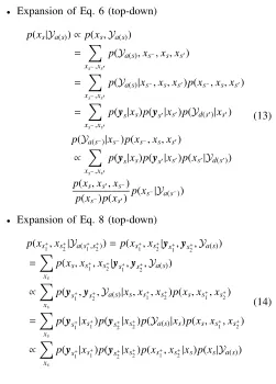
• Expansion of Eq. 6 (top-down)
p(xs|Ya(s))∝p(xs,Ya(s))
= X
xs−,xs′
p(Ya(s),xs−,xs,xs′)
= X
xs−,xs′
p(Ya(s)|xs−,xs,xs′)p(xs−,xs,xs′)
= X
xs−,xs′
p(ys|xs)p(ys′|xs′)p(Yd(s′)|xs′)
p(Ya(s−)|xs−)p(xs−,xs,xs′)
∝ X
xs−,xs′
p(ys|xs)p(ys′|xs′)p(xs′|Yd(s′))
p(xs,xs′,xs−)
p(xs−)p(xs′)
p(xs−|Ya(s−))
(13)
• Expansion of Eq. 8 (top-down)
p(xs+
1,xs
+
2|Ya(s
+
1,s
+
2))=p(xs
+
1,xs
+
2|ys+1,ys
+
2,Ya(s))
=X
xs
p(xs,xs+
1,xs
+
2|ys+1,ys
+
2,Ya(s))
∝X
xs
p(ys+
1,ys
+
2,Ya(s)|xs,xs
+
1,xs
+
2)p(xs,xs
+
1,xs
+
2)
=X
xs
p(ys+
1|xs
+
1)p(ys+2|xs
+
2)p(Ya(s)|xs)p(xs,xs
+
1,xs
+
2)
∝X
xs
p(ys+
1|xs
+
1)p(ys+2|xs
+
2)p(xs
+
1,xs
+
2|xs)p(xs|Ya(s))