SEASONAL TRAVEL DEMAND AND PEAK LOAD
PRICING ON THE
AUSTRALIA-U.S.A. AIR ROUTE.
by
T. LEETAVORN
Submitted in partial fulfilment of
the requirements for the Master of
Transport Economics degree.
THE UNIVERSITY OF TASMANIA
AUGUST
1982
This dissertation represents my own original.
work and contains no material which has already
been published or otherwise used by me, and
to the best of my knowledge it contains no copy
or paraphrase of material previously written by
another person or authority, except where due
acknowledgement is made.
ACKNOWLEDGEMENTS
I would like to acknowledge the assistance
of my supervisor Professor J.H.E. Taplin, whose
advice and encouragement helped me complete this
dissertation.
I would like to thank Mr. D. Challen, who helped
me set up the econometric model. Finally, Ms. M.
CONTENTS
Page No.
_INTRODUCTION
0 0 0 0 0 1CHAPTER 1:
THE INTERNATIONAL AIRLINE INDUSTRY
A)Operational Framework
5
B)Capacity and Tariffs
008
C)Costs
10
CHAPTER 2:
EFFICIENCY AND PEAK LOAD PRICING
13
A) Peak Load Pricing
14
CHAPTER 3:
THE AUSTRALIA-U.S.A. PACIFIC ROUTE
19
CHAPTER 4:
SOME CHARACTERISTICS OF THE INTERNATIONAL
LEISURE TRAVELLER
0 022
A)The Motivation and "Pull" Factors ..
24
B)"Push" Factors
25
C)Demand Studies
S O28
CHAPTER 5:
MODEL SPECIFICATIONS AND DATA
..
39
A)Single Equation Specification
..
40
B)The Data
..
47
CHAPTER 6:
THE RESULTS OF THE SINGLE EQUATION
ESTIMATION
0 051
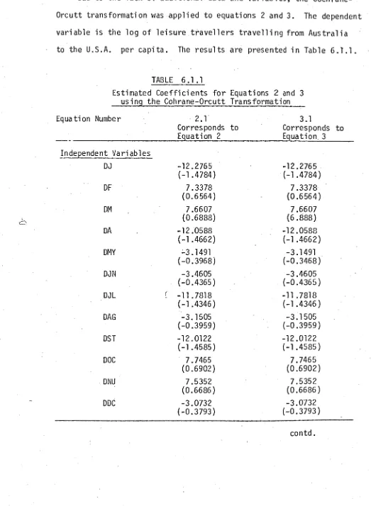
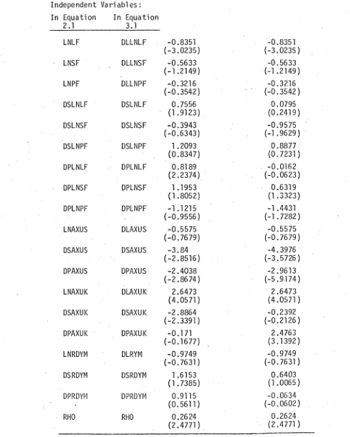
A) Results of the Cochrane-Orcutt
Transformation
59
CHAPTER 7:
A COHERENCE APPROACH TO ESTIMATING THE
PRICE ELASTICITIES FOR THE DEMAND FOR
LEISURE TRAVEL BY TRAVEL SEASONS
66
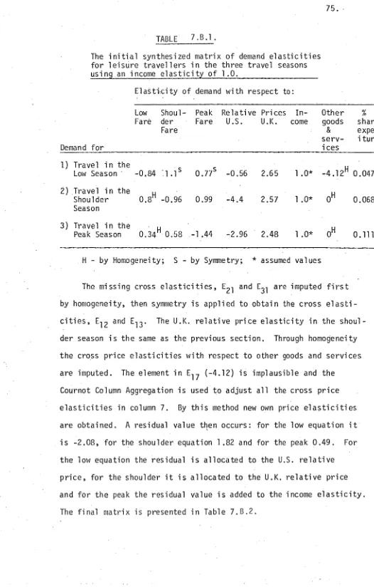
A) The Synthesized Matrix of Elasticities
V.
Page No.
B)Sensitivity Tests - Using an
Income Elasticity of one •• 74
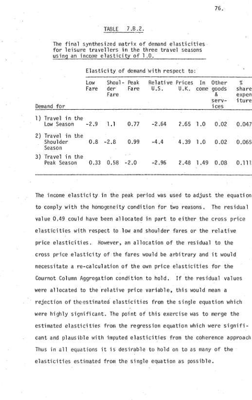
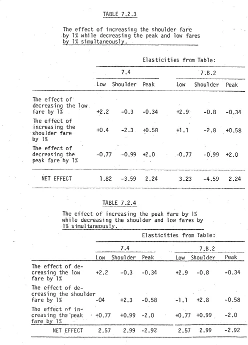
C)Net Effects • • 77
CHAPTER 8: PEAK LOAD PRICING ON THE AUSTRALIA-U.S.A.
AIR ROUTE 82
A) Calculation of the Optimal Fares 83 B) Costs
(i)Short run marginal costs 88 (ii)Long run marginal costs 90
C) Policy Implications 90
APPENDIX A.
APPENDIX B.
APPENDIX C.
APPENDIX D.
APPENDIX E.
APPENDIX F.
APPENDIX G.
APPENDIX H.
APPENDIX J.
APPENDIX K.
BIBLIOGRAPHY
Synthesized Matrix of Elasticities of Demand for Categories of Vacation Travel and Tourist Accommodation:
Australian travellers 95
Separate Equation Results 96
Interpolation of the Population Figures 100
Construction of the Relative Prices
Variable 103
Raw Data , 108
Calculation of the Price Elasticities .. 121
Correlation Matrix for Equation 2 .• 122 Correlation Matrix for Equation 3 126
Calculation of Expenditure Shares 130
Calculation of Optimum Fares .• 133
Calculation of the Individual Effects of
Since the early 1970's international travel and tourism have
become important issues to many governments and of course the airline
operators who have had to contend with rapidly rising costs of
opef'a-tions and capital. To some extent this problem has been alleviated
through rapid technological advances made in the aviation industry.
At the same time the airline operators have become aware of the
leisure travel market which throughout the mid to late 1970's has
provided the airlines with a boom period. This boom is slowly tapering
off at a time when major carriers have just completed a re-equipment
phase aimed at a growing market; pricing strategies have become an
increasingly important tool for the operator to increase utilisation
of their capacity.
Many researchers have used econometric techniques for estimating
airline demand functions, from these studies aggregate fare elasticities,
different fare class elasticities, income elasticities and other
ser-vice elasticities have been estimated. Each of these studies has shown
the importance of fare and income elasticities in the leisure travel
market. These basic estimates have helped to form some useful pricing
policies. Recently operators and policy makers have noted the
varia-bility of demand for travel over time; as supply is fixed in the short
run, operators have experienced periods of excess supply and periods
of excess demand. To combat this variability of demand over time,
operators have introduced seasonal pricing. As this is a recent
inno-vation, no research work has been done on estimating the cross
relation-ship between travel seasons. This study attempts to estimate the cross
relationship between travel seasons on the Australia-U.S.A.-Pacific
2.
Seasonal and directional imbalances were cited by the Review
Committee on Australian international civil aviation policy as being
one of the major problems facing airline operators operating to and
from Australia. Seasonal demand imbalance refers to the fact that
travellers have preferred months of travel, which tends to lead to.
periods of high demand being concentrated into a few months of the
year. Directional demand imbalance refers to the growing disparity
between arrivals and departures into Australia. Figure 1 highlights
both seasonal and directional demand imbalances. For Australian leisure
travellers travelling to the United States the peak months are May,
June, August and December. ' The off-peak months are February, March,
October and November and the official shoulder months are January,
April, July and September. While for travel from the U.S.A., the
peak months are August, September, October and January; the shoulder
months are February, July, November and December and the Off-peak months
are March, April, May and June. Seasonal demand imbalance focuses on
travel in one direction, while the directional imbalance focuses
attention on travel in both directions. For instance, a good example
of the directional imbalance problem is that the peak travel months
for Australians going to the U.S.A. are May and June, which are the
off-peak travel months for Americans visiting Australia. Both these
imbal-ances create problems of which capacity utilisation is a major one.
In 1979 the operators on the Australia-U.S.A. route made a
conscious attempt to smooth out demand. They introduced seasonal price
variations on the advanced purchase fare (APEF), the Group inclusive
air fare (G.I.T.) and the Budget fare. The effects of these fares can
be seen in Figure I. for true origin destination leisure travellers on
the route for 1979 to 1980. The results are still unclear, but there
77V
it
l€
'/LEAS
—'
— .AL141
.
:
:#41411
.41IS
i
i
:
FIGURE 1.
LEISURE TRAVELLERS, AUSTRALIAN TRAVELLERS TO THE U.S.A. AND AMERICAN TRAVELLERS
_
TO AUSTRALIA..
'
I ' '
rkbIL)/1- 70
- ,
- 14k
.A
.
tr
• •-j • ....
Tr
av
el
1
ers
• A j
1.1 1..! • 1
: i
■
; II ..I :.; .
.,,•
F PIA 1717.TA ONDSF 014 reki..34.SOMO.7: f.trA P1J JA--SOit1DJ-Ft))6• 013.3/9-$"0/0D/Frnil•-r0,5ZA • s..04)C,J Fr:IA.1)1S 3.A-soN.D :.3" p,plft z aerc °Arts i
• - I' lq75- IL; 1776 I • • L-P77
• ILLLLLAN •
• •1
/
T
A
T
- ••
f
i
t
0.
I - •/
97i
time •
4.
appears to be a reduction in travel in the peak (Australia to U.S.),
while off peak travel seems to be increasing in both travel directions.
This study estimates the cross relationship between travel
seasons using the ordinary least square technique. The results from
the model will be used to determine the optimum level of fares for
5.
CHAPTER 1.
THE INTERNATIONAL AIRLINE INDUSTRY
A.
OPERATIONAL FRAMEWORK
Commercial aviation grew strongly after World War II, with two
nations being primarily responsible for setting up the operational
frame-work of the industry; they were the United States and the United
King-dom. These two nations had opposing views, the United States favoured
an open skies policy while the United Kingdom favoured regulation in the
form of strict capacity limits. The 1946 Bermuda agreement between the
two nations saw a compromise of opposing views, but more importantly
set up a framework for an exchange of landing and traffic rights, the
basis of a bilateral agreement.
Prior to the 1946 Bermuda agreement, two basic freedoms for
inter-national airline operators were drawn up at the 1944 Chicago Convention.
These freedoms were:1
FIRST FREEDOM: the privilege to fly across a contracting
party's territory without landing, and
SECOND FREEDOM: the privilege to land for non-traffic
purposes (i.e. refuelling and maintenance).
A further three freedoms were drawn up at the 1946 Bermuda agreement:2
THIRD FREEDOM: carrier has the privilege to put down
passengers,mail and cargo originating from its own territory,
FOURTH FREEDOM: a carrier of a contracting party has the
privilege of picking up passengers, mail and cargo destined for its home country.
1. Report of Review Committee,
Review
of
Australian International
Civil
Aviation Policy,
2 Vols., (Canberra, A.G.P.S., 1978) Vol. 1, fy.5.Nation
Nati on Freedom
6.
FIFTH FREEDOM: a carrier has the privilege to take on passengers, mail and cargo destined for the territory of any other contracting state. It also has the privilege to put down
passengers, mail and cargo originating from any of its other contracting states.
The intent of the third, fourth and fifth freedoms may be made clearer
by the following diagram.
DIAGRAM I.
A diagramatic representation of the third, fourth and fifth freedoms,
based on airline domiciled in Nation A.
FREEDOM 3
Nation A FREEDOM 4
FREEDOM 5
Nation
A Nation
Nation
Nation
A — 3 — Freedom — 5 — Freedom
Nation
Source:
Report of Review Committee,Australia's
International Civil Aviation Policy,
(Canberra, A.G.P.S., 1978), Vol. I, P-6.
Thus on the Australia-U.S.A. air route, the bilateral agreement allows for the Australian designated carrier (Qantas) to take passengers from Australia to the U.S. (third freedom). The fourth freedom gives Qantas the right to pick up Australia bound passengers from the U.S. The
.
To these basic freedoms there should be added the so-called
sixth freedom. This freedom refers to the situation where the designated airline of one state Party to an agreement carried traffic between the grantor state's territory and that of a third state, with a stop in the airline's home territory. This sixth freedom is a mixture of the third and fourth freedoms, this can be seen in diagram-2.
DIAGRAM 2.
A diagramatic representation of the "sixth freedom", based on airline domiciled in Nation A.
SIXTH FREEDOM
1
[Nation Nation Nationl >
I Freedom 4 A Freedom 3 C
Source:
Report of Review Committee,Australia's
International Civil Aviation Policy
(Canberra, A.G.P.S., 1978), Vol.1, P-6.
As Australia is usually .a terminal point for air services, transit traffic is small and sixth freedoming by other carriers may only be negligible. An example of sixth freedoming on the Australia-U.S.A. Pacific route is as practiced by Air New Zealand. Travellers bound for the U.S. are picked up by Air New Zealand, flown to Auckland and then to the U.S.
8.
Transport Association's (I.A.T.A.) failure to carry out its main role,
that is as a fare setting body.4 At these, fare setting conferences
I.A.T.A. had to reconcile the very different positions among carriers:
each carrier had its own cost function on which it wanted to base its
fare, and secondly, the motivation behind most of the carriers was the
5 achievement of government set objectives.
Thus the bilateral agreements dictate the operational environment
between the two contracting states. The most important matters covered
in a bilateral are the fare to be charged and the operating capacity
and its adjustment mechanism. 6
B.
CAPACITY AND TARIFFS
An air services agreement between Australia and any other
contract-ing state would eventuate if there is sufficient true origin and
destin-ation traffic on the proposed route.7 The volume of true
origin-destin-ation traffic would also determine the level of capacity offered. Once
capacity has been determined, flight frequency is also determined.
The Australian policy on capacity has been to allow the
predeter-mined capacity level to be modestly in excess of the anticipated demand
for travel.8 If the underutilised capacity is minimal, the carrier's
unit cost of production would fall and it is part of the Australian
policy to attempt to ensure low cost travel to Australian consumers.
In most bilateral negotiations, attempts are made to split the
4. M.R. Straszheim,
"The International Airline Industry"
(WashingtonD.C., The Brookings Institution, 1969), p. 33.
5.
Ibid.,
p.6. Report of Review Committee,
Australia's International Civil
Aviation Policy
(Canberra, A.G.P.S., 1978), p. 9.7.
Ibid.,
p. 8.T.O.D. traffic between the two carriers. Thus the capacity level
offered by each carrier would approximately be enough to satisfy half
. of the market demands. At all times traffic levels are monitored. I
most agreements there is a trigger mechanism which allows upward
adjust-ments of capacity once a certain level of traffic has been achieved.
On the Australia-U.S. route there is more flexibility with regards to
capacity adjustments: capacity can be adjusted upwards or downwards
with only the approval of the originating country's regulatory body
being necessary. After a period of six months the effects of this new
level of capacity is reviewed.9
The level of fares offered on the routes will affect capacity
utilisation on the route. Most fares have to be agreed upon by both
contracting states, along with any subsequent fare changes. However,
on the Pacific route in 1978 an amendment was made regarding fares,
giving either party the right to introduce new fares without the other
party's approval.10 The effects of the new fares are subject to review
after six months.
Schedule operators have maintained that at any point in time
capacity must be greater than demand. The reasons are.:11
(a) maintenance of departure time flexibility,
(b) multi-stop services face varying traffic direction, and
(c) variations in time and direction are inevitable
concomittants of demand.
9. Unfortunately, the libraries do not hold the original 1946
bilateral agreement between Australia and the U.S. The source of this information was Prof. J.H.E. Taplin, and was verified by the D.O.T., Canberra.
10. Australian Treaty Series,
Amendment to the Air Services Agreement
with the United States
(Canberra, A.G.P.S., 1980), No. 2.11. Report of Review Committee,
Review of Australia's
10.
Another factor that has affected capacity has been the rapid
techno-logical advances made within the aviation industry, particularly the
introduction of wide-bodied jets. The use of wide-bodied jets has
affected scheduling flexibility, firstly as capacity has become more
concentrated, the number of planes required to service a route (assum-
ing no increase in demand) will be reduced which reduces flight frequency.
Secondly, operators are reluctant to reduce frequencies as it may reduce
their market shares. This suggests the operators believe the frequency
elasticity to be at least one. However research has shown frequency
elasticity to be below one. Ippolito estimated a frequency elasticity
for some U.S. domestic routes to be 0.864. 12 If flight frequency were
reduced by 1% this would lead to a reduction of patronage by 0.864%.
Thus a reduction in the level of frequencies offered may not lead to a
more than proportionate decrease in patronage.
C.
COSTS
To determine the appropriate fare structure, the operator must
have some understanding of the structure of costs. Financially, an
airline's cost of production is influenced by: 13
(a) distance,
(b) aircraft size and speed,
(c) utilisation, and
(d) tangible aspects of service quality.
The items listed above affect mainly the airline operating costs.
The route network of an airline will determine its cost structure.
Different aircraft are designed for different stage lengths and by
care-fully matching the equipment with the route network the operator may
12. A.I. Ippolito, "Estimation of airline demand with quality of
service variables",
J.T.E.P.,
Jan. 1981, p.13.13. G.N. Douglas and J.C. Miller, Economic Regulation
of
Domesticaircraft is found to decrease with distance up to a certain point. The
decreasing cost per passenger is due to the fact that a
disproportion-ately large share of fuel is consumed during the take off. 14 Further,
the crew and aircraft time in the take off and landing processes are a
fixed cost which can be spread over more miles as the stage length
increases.15 There may also be some economies of scale associated with
aircraft size: equipment and crew costs do not increase proportionately
with increased capacity. 16
Three other major categories of costs are ownership cost of
capital (principally aircraft), passenger and flight traffic costs and
overhead expenses. The largest share of the cost of operating a
scheduled air transport system is the cost of generating capacity,
specifically operating costs and ownership cost of capital. ]7
The regulatory environment is of particular interest: if the
air-lines were allowed to compete freely, management would be forced to
become cost-conscious and only efficient carriers would survive. At 18
present the international airline industry is regulated, probably
allowing inefficient carriers to continue to exist.
As noted above, by matching the equipment to the route
character-istics, airlines can achieve significant cost savings. Per passenger
cost can be lowered further by increasing the load factor, resulting in
operating costs and fixed costs being spread over more passengers. In
14. M.R. Straszheim,
The International Airline Industry,
1969, p. 85.15.
Ibid.
16.
Domestic Air Transport Policy Review,
2 Vols. (Canberra, A.G.P.S.,. 1979), Vol. 2, p. 12.17. G.N. Douglas and J.C. Miller,
Economic Regulation of Domestic
Air Transport: Theory and Factice,
p. 7.12.
the short run capacity is fixed and cannot be stored while demand is
variable over time. If one fare level is used this would create an excess
of demand and supply at various times of the year due to the season-
ality of demand. In the peak season (usually the summer months) there
may be an excess of demand over supply in which case each seat acquires
a rental value and the fare should reflect this. In the off-peak season
(usually the winter months) the reverse occurs and there is no rental
value to charge the users. Intuitively, fares should be varied between
season; this may discourage some peak travellers while encouraging a
greater use of the capacity available in the off-peak. The general
result is a smoothing of the peaks and troughs, leading to a higher
CHAPTER 2.
-
EFFICIENCY AND PEAK LOAD PRICING=In the previous chapter it was shown that the demand for travel
is subject to seasonal movements. Variation in travel demand occurs
throughout the year, the day of. the week and the time of. the day; thus
at certain periods the resources available are underutilised; this -
imposes additional cost to both the users of the facility and the
producers. Peak load pricing could provide a. solution that would
improve capacity utilisation, while making travel available to a greater
proportion of the public.
Peak load pricing becomes feasible when demand varies with time
and a common supply system is used in the peak and off-peak periods)
The solution sought is one which reflects the cost at various times and
simultaneously discourages consumers from overloading the system when
it is used most intensively (i.e. in the peak periods). 2 The effect
of peak load pricing is not necessarily to eliminate growth in the peak
period, but to set prices which reflect costs and provide consumers
with the correct signals to enable them to take into account the
conse-quences of their increased demand on the system. 3
The role of pricing is twofold, firstly: it has a role of
directly allocating resources efficiently. Secondly, it provides a
signal to invest.4
1. C.M. Price,
Welfare Economics in theory and practice
(Macmillan, London, 1977), p. 139.
2.
/bid.,
p. 139.3. .R. Turvey and D. Anderson,
Electricity Economics
(JohnHopkins, University Press, Baltimore, 1977), p. 71.
4. J.J. Warford,
public Policy Towards General Aviation
(Washington14.
A.
PEAK LOAD PRICING
The transport industry is typified by a demand that tends to
vary with time and a common supply system that is fixed in the short to
medium term. In the airline industry, capacity is fixed in the short
run through bilateral agreements and fares are also fixed in the same
manner. However, the Australian government does encourage the use and
development of promotional fares. Thus there is some scope for
flexi-bility in this area. Adopting an incorrect price set in this situation
could lead to poor aircraft utilisation and wrong investment decisions.
Assuming the authorities are concerned with maximising social
welfare, the following pricing strategy should be adopted to equate
price to marginal cost. For ease of exposition it is assumed that first
best conditions are prevalent. It is also assumed that there are only
two demand periods in a year, the peak period lasting two-thirds of the
year and the off-peak period lasting the remaining third of the year.
Further, the two demand periods are independent of each other.
The basic rule for peak load pricing is to set the price in
each demand period to its corresponding short run marginal cost with
the investment decision being based on the long run marginal cost. The
short run marginal cost consists of the operating cost, while the long
run marginal cost consists of both the operating cost and the capacity
cost. Following the general rule the off peak price would generally
be below the long run marginal cost while the peak price would be above
the long run marginal cost. This effect can be seen in diagram 11.1
where the capacity costs are p, per unit per period, the operating costs
are b per unit per period and the plant is assumed to be completely
divisible.
Diagram II.
SRMC1
- Q12
Source:
O.E. Williamson, "Peak load pricingand optimal capacity under indivisibility
contraints". A.E.R., Vol. 36, Sept. 1966, p. 818.
The operating cost is assumed constant at b per unit. When capacity
Ql is reached, the short run marginal cost (SRMC) becomes vertical.
SRMC1 and LRMC1 correspond to the capacity available at Q1 , while SRMC2
and LRMC2 correspond to the capacity available at Q2. The off peak
demand curve, D1 , interests the SRMC1 at Pll . The peak demand curve
D2, interest SRMC2 at P21 ; then P11 and P21 are the appropriate prices
to levy during the off-peak and peak respectively. The justification is
16.
the periods.
Intuitively, capacity is set to meet the highest level of demand. In the airline industry capacity is determined by the volume of true origin-destination traffic. The largest cost item for the airline industry is the cost of providing that level of capacity, once that capacity level is fixed and operational; operating outside the peak period would only incur the operating expenses. Thus as long as the operating cost is covered, it would be beneficial for the operator to maintain those services in the off peak.
This pricing strategy has often been confused with price discrimin-ation. The two cases may be distinguished by looking at the marginal opportunity cost. A discriminating monopolist charges different prices
to different consumer groups, however all consumers are served at the same marginal opportunity cost.5 That is the value of the. first unit of unsatisfied demand in the higher priced market is the most valuable alternative foregone.6 In the peak pricing case, taking a unit away from the off peak period does not make it possible to supply a unit on-peak. Thus the higher on-peak value is not the relevant alternative social opportunity cost for the off peak demand.7 Thus the marginal opportunity is different for both periods.
The construction of the effective demand curve (DE) allows the optimum plant size to be solved for geometrically. In diagram 11.2 the effective demand curve is obtained by taking the vertical difference between the periodic load curve and the SRMC(b), multiplying the differ-ence by Wi (the fraction of the cycle during which load i prevails) 5. J. Hirshleifer,"Peak Loads and Efficient Pricing: Comment",
Quarterly Journal of Economics,
Vol. 71, 1958, p. 549.and adding vertically their weighted demand for capacity curve to
SRMC.8 To match total revenue (Pi Qi Wi) to total costs (b Q. W. + the price charged must equal Pi = b + 0/W1. The effective demand curve is constructed in such a manner that it intersects the LRMC at the
capacity level Qi, corresponding to the price b + f3/Wi.9 The intersection of the effective demand curve and the LRMC determines capacity. By
setting the price at the intersection of the SRMC both the respective
periodic load demand curves will ensure that net revenue is zero (i.e.
(b
1
3
1)P
ll 2[1321 - (b +f31)]*. Thus the amount by which revenue in the off-peak fails to cover pro rata the total cost, is precisely off-set by the revenue obtained in the peak period.If the capacity costs ge-rei32 per unit per period, LRMC intersects DE at G, thus the optimum plant size is Q2. The prices are P12 and P22 in the off-peak and peak periods respectively. The kink at F in
diagram 11.2 indicates that the demand price along the off peak curve is everywhere below the SRMC.
This pricing strategy allows higher utilisation rates in the off peak and eliminates consumers from overloading the system in the peak. It should be noted that peak load pricing is not an attempt to eliminate
growth in the peak period, but to pass on the correct signals to the
consumer by making them aware of the costs they cause by travelling in
the peak.10
If a uniform pricing strategy were adopted it could leadto a growth in consumption at the peak periods which may result in
additional investment in that good at the expense of alternative project
8. O.E. Williamson, "Peak Load Pricing",
A.E.R.,
Vol. 56, Sept., 1966, p. 817.9.
/hid.,
p. 818.18.
developments.
As noted earlier, this exposition of peak and off-peak pricing
has been based on the assumption of independent demands in the two
periods. In fact, high and low season demands for overseas travel are
not independent, and a major objective of this study has been to quantify
the interrelationship between high, shoulder and low season demands.
As will be shown in Chapter
8,
the solution to the problem is morecomplex whenall of the cross-relationships are known, but the basic
CHAPTER 3.
THE AUSTRALIA-U.S.A. PACIFIC ROUTE
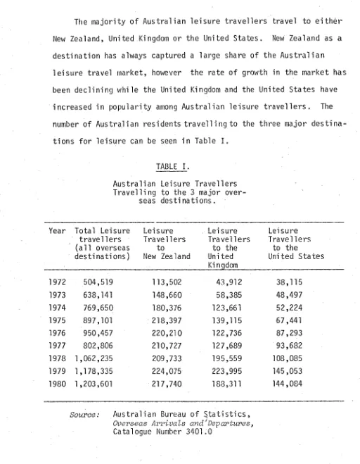
The majority of Australian leisure travellers travel to either New Zealand, United Kingdom or the United States. New Zealand as a
destination has always captured a large share of the Australian
leisure travel market, however the rate of growth in the market has been declining while the United Kingdom and the United States have increased in popularity among Australian leisure travellers. The
[image:24.559.30.542.149.808.2]number of Australian residents travelling to the three major destina-tions for leisure can be seen in Table I.
TABLE I.
Australian Leisure Travellers Travelling to the 3 major
over-seas destinations.
Year Total Leisure travellers
(all overseas
destinations)
Leisure Travellers
to
New Zealand
Leisure Travellers
to the United Kingdom
Leisure Travellers
to the
United States
1972 504,519 113,502 43,912 38,115
1973 638,141 148,660 58,385 48,497
1974 769,650 180,376 123,661 52,224
1975 897,101 • 218,397 139,115 67,441
1976 950,457 220,210 122,736 87,293
1977 802,806 210,727 127,689 93,682
1978 1,062,235 209,733 195,559 108,085
1979 1,178,335 224,075 223,995 145,053
1980 1,203,601 217,740 188,311 144,084
Source:
Australian Bureau of statistics,20.
The figures in Table I only include short term movements, which is
defined as a length of stay away from Australia being less than twelve
months. They are true origin-destination figures.
The capacity provided by the airlines on the Australia-West Coast
U.S.A. route for 1980 was 17 Boeing 747's per week.' This amounted to
approximately 6,375 seats in either direction. This level of capacity
is offered all year round; thus, the total number of seats available
for 1980 was 331,500.
TICKET TYPES
The Australian government has pursued a policy of encouraging
scheduled carriers to develop a range of promotional fares. 2 Increased
fare flexibility allows the carriers to encourage travel from
differ-ent market segmdiffer-ents. If the fares and conditions of travel closely
match the requirements of the traveller, this could lead to a growth
in traffic. This growth in traffic could (if it does not require a
proportional increase in capacity) lead to a decrease in per passenger
costs.
Since 1970 on the Australia-West Coast U.S.A. route three major
types of tickets have been available to the traveller. 3 The first
two fares are the normal first class and economy class fares, these
fares are free of any restriction. The third fare type is the advanced
purchase fare (APEF) which was introduced on to this route in September
1973. The conditions attached to this fare are a minimum of length
of stay in the destination country, no stop overs and payment for the
ticket to be made 45 to 60 days in advance of the departure date.
1. Source: Qantas.
2. Report of Review Committee,
Australia's International Civil
Aviation Policy,
Vol. 1, p. 24.• This fare offers savings to the traveller at all times of the year
when compared to other fares. The advantages that accrue to the
carrier are that they would be able to plan with more certainty if
bookings are made in advance. Secondly the carrier has full access
to payment in advance which reduced the problems of no-shows (penalties
are attached on not travelling at the agreed time). Finally stop
overs cannot be made, this reflects the economies gained by the
car-rier if the passenger travels end to end.
In February 1979, the airlines introduced seasonal pricing and
applied it to the APEF fare. Thus if the potential traveller chooses
to travel in the off peak travel season, he would save a considerable
amount when compared to travelling in the shoulder or peak season.
This pricing strategy was adopted in the hope that it would direct
price sensitive travellers and potential travellers to change their
22.
CHAPTER 4.
SOME CHARACTERISTICS OF THE INTERNATIONAL
LEISURE TRAVELLER
Travel demand studies have distinguished between two main travel
purposes, that is travel for business and travel for leisure.
Busi-ness travel has been seen to be motivated by increasing sales, and
time is an important constraint to the business traveller. Leisure
travel is discretionary travel; time of departure and arrival are not
as important to the leisure traveller compared to the business man.
Thus the type of service required by the two categories would tend to
differ. Because of the time constraint the business traveller
re-quires an on-demand service. He also rere-quires a greater degree of
comfort than the leisure traveller. Presumably if a businessman is
to successfully conduct his business in distant places, his trip
should be made as comfortable as possible. The businessman's
on-demand service requirement also places an obligation on the carrier
to provide a wide range of destinations, departure times (days of
the week and time of day); the service must also be reliable.1
It has been observed that the leisure traveller is generally
prepared to trade off lower fares for his comfort and generally lower
product requirements. Qantas, in a report released in 1977, used
factor analysing to separate out two market segments against the
pro-duct features.-,_The results are present in Table 4.1. This analysis
shows that there is a distinct diffei-ence in the product requirement
for the two segments. Segment A can be said to represent the business
traveller, while B represents the leisure traveller.
1. Qantas,
A Review of International Air Services to and From
Australia,
Submission to the House of Representatives Select Committee on Tourism, 1977.TABLE 4.1
Qantas Analysis on Market Segments
Product Feature Market Segment
A
Flexibility High None
Choice of Destination High None
Choice of Time High None
Choice of Day High Low
Reliability High Moderate
Comfort High Low
Source:
Qantas 1977.A Review of International Air
Services to and from Australia.
Submissionto the House of Representatives Select Committee on Tourism.
Generally, the socio-economic characteristics of the two cate-gories of travellers are different. The typical business traveller is male, middle aged and his income is usually high.3 The leisure traveller exhibits a double hump age distribution, coming from the under 25 and over 50 age groups.4 The income levels are usually low for the under 25s and moderate to high for the over 50s age group.
The differences presented here suggest that for-modelling pur-poses the two types of traveller should be segregated and their travel behaviour should be modelled independently. This approach has been adopted by most of the recent studies in the area of travel demand
24.
estimation.5 This study concentrates on estimating demand for travel by leisure travellers. Many factors influence the decision to travel,
broadly speaking these factors are part psychological (e.g. the weather) and institutional (e.g. leave periods). The psychological
factors tend to make up the "pull" factors that motivate people to travel. Changes in institutional factors directly induce either
increases or decreases in travel; these are termed "push" factors.
A.
THE MOTIVATION AND "PULL" FACTORS
The motivation for leisure travel is a complex area, which is not easily modelled. Some insight can be gained from social scientists
who have attempted to explain the phenomenon.
Travel is.a derived demand. Few fly from A to B simply for the sake of 'flying, thus destination choice is important. In choosing a
destination, the traveller would rely on his previous experience, the type of recreational facilities available at the destination, the hours of daylight, temperatures and the number of days Of rain.6 How
much these factors influence travel behaviour is still unknown, however, it is undeniable that the above factors enter the traveller's frame
of reference when deciding on a destination.
The need to travel also arises from the tourists' subjective needs. First, there is a need to relax, to escape from physical fatigue and nervous tension.7 Secondly, there is a need to change
the daily routine and to enjoy some of the rewards of earning a living.8 Thirdly, there is a need to escape from the constraints, for which
physical distance from normal surrounds is required.9
5.. See Smith & Toms, M.R.-Straszheim (1972),Edwards (1979), Oum Gillen (1980), in Chapter 4.C.
6. European Conference of Ministers of Transport,
Holiday Traffic
(Paris, 1978), No. 4, p. 10.7. /bid.
9./bid.
The existence of these factors shows that there is a desire to
experience new things and a general desire to get away. These
desires can be fulfilled by travelling. Without these "pull" factors,
changes in the "push" factors would have a very small effect on the
growth of travel.
B. "PUSH" FACTORS
The push factors, outlined below, directly induce increased travel,
by generation or by increasing the frequency of travel. 10
(1) population growth and structure,
(2) income growth,
(3) income distribution between socio economic groups,
(4) general rate of domestic inflation,
(5) changes in the relative price of major items on which
income may be spent,
(6) changes in periods of annual leave entitlements,
(7) facilities for domestic tourism and their prices,
(8) facilities for and the price of holidays abroad,
(9) new attractions for tourists, home and abroad,
(10) promotions and marketing of tourism at home,
(11) promotions and marketing of tourism abroad,
(12) social and other forces affecting consumer preference
for spending income.
Most of the effects of the-factors outlined above on travel are
obvious. For instance as the population increases, it would be
expected that the number of travellers would also increase. The
popu-lation structures would also affect travel: if there are large numbers
10. A. Edwards,
International Tourism Development Forecasts to
26.
of elderly or very young people in the population, this could lead
to a decrease in the number of travellers.
The length of annual leave periods and how they are taken would
affect the type of travel, that is domestic versus international.
The average length of paid annual holiday in Europe, U.S. and Australia
is 41/2weeks .11 Obviously the longer the period of paid annual holidays,
the easier it becomes formorkers to travel abroad.
However, recent trends have been towards decreasing the working
week and tying in public holidays with weekends. The increase in
leisure time in this manner would decrease the level of international
travel as the time constraint reduces the number of destinations.
Income growth and its distribution among socio economic groups
would also have an effect on travel. Travel has generally been
accept-ed as a luxury good. Thus, as income increases, the number of leisure
trips taken would also increase. Eventually a saturation point will
be approached, and further increase in income would lead to a slower
rate of increase in the demand for travel. This effect is shown in
figure 4.1.
FIGURE 4.1
SATURATION EFFECT
\0
>
M W S- 0-
4- E
0
-1-) W
M E = 0 Cr.r-
S- W M
0
F- A
Household disposable income
Source:
Edwards, R.,International Tourism Development
Forecasts to 1990,
p. 37.Figure 4.1 shows clearly that as disposable income increases, the quantity of tourism per period of time consumed increases at an increasing rate (A to B range), after which (at C) the rate of increase
in consumption declines. This general pattern hides the effect of income distribution among socio-economic groups. Obviously disposable
income levels are not the same for all households, thus the
responsive-ness of travel to their level of income would be different. For American travellers in 1975, G. Newman estimated income elasticities with respect to travel for different income classes. The results
were:
TABLE 4.2.
Income Elasticity by Income Classes
Income, $'5000: up to
$5 $5-10 $10-15 $15-20 $20-25 $25-50 $50+
Elasticity 0.7 1.4 2.1 3.7 3.4 1.5 1.1
Source:
Newman, G., ."Forecasting at Pan Am",fromAllanagement of Tourism,
p. 216.Clearly the rate of increase in household disposable income and the distribution of income are important variables that should be
deter-mined for forecasting future travel.
The rate of domestic inflation would affect the level of dispos-able income. The rate of inflation at the country of destination'
could also affect its relative attractiveness compared to other possible destinations.
28.
interest and the mix in the consumption bundle.- When looking at
international travel, a likely alternative is domestic travel.
One factor not yet explicitly mentioned is the price of travel.
The proportion of total tourist expenditure spent on travel has been
estimated by Wheatcroft to be approximately 40%, being a major
compon-ent of tourist expenditure. Any variations could lead to changes in
destination, postponing travel or not travelling at all. The usual
relation between price and demand is inverse; the higher the price
the lower the demand. The prices of other goods and services affect
the demand for tourism through their effect on general expenditure,
thus a tourist may choose a less expensive form of tourism to have a
greater amount available to spend on other items.12 This tendency
is particularly strong in the case of goods with a strong complement
or substitute of another good. For instance the demand for a
particu-lar form of tourism may increase if offered in conjunction with a
lower air fare. On the other hand, in the case of substitutes a fall
in the price of a tour package may lead to a fall in demand for a
competing package.
All these factors have provided the "push" for travel. How
researchers have managed to model the demand for leisure travel will
be seen in the next section.
C.
DEMAND STUDIES
Past researchers have mainly used the ordinary least squares
technique to estimate airline demand functions. In the modelling of -
air travel demand they appear to have been constrained by data which
has limited the number of independent variable specified in. the model.
12. B. Archer, Demand
Forecasting in Tourism,
Bangor OccasionalThe two basic variables that have been used in air travel demand models
are the fare and some measure of income. Other variables have been
added to this basic model such as a time trend variable and an
exchange rate/relative prices variable.
The effects of the fare and income on demand for air travel is
well known. The time trend variable was included to capture the effect
of changing technology: in view of the rapid technological advances
made in the airline industry (e.g. wide-bodied jets) a time trend
vari-able would seem to be appropriate. However, the trend varivari-able may
also pick up other effects: such as increases in population, and
in-creases in real income over time. This effect would tend to mask the
individual effects of other variables included in the model.
Straszheim (1969) estimated the demand for air travel across the
North Atlantic from 1954 to 1964 using annual data. He adopted the
following specification:13
Ln T
2 R
where: =
=
6.5496
0.9971
0.3157 Ln Price - 0.7613 Ln Income
(1.2308)* (1.538)*
0.1825 time (7.9694)*
Ln T = the log of all travellers from New York to London, Ln Price = the log of the real New York to London fare,
Ln Income = the log of income, Time = time trend.
The only significant variable in this model was the time trend;
neither the pricenor income coefficients were significant. The income
coefficient was negative, thus it was unacceptable. The sign problems
and the low t-statistics on the price and income variables would be
13. M.R. Straszheim,
The International Airline Industry
30.
due to a high correlation between the fare and income variables.
Possible solutions to breaking the correlation among the
independ-ent variables are to include more variables into the model, increase
the number of observations or take first differences of the data.
Brown and Watkins (1968) used the same variables as Straszheim •on U.S.
domestic air travel but took first differences in logs of the data. 14
They used annual data from 1946 to 1966; the results were: 15
A
Ln T = 0.0725 - 1.307A
Ln F + 1.119A
Ln Y 0.038 Ln T(4.491) (2.922) (10.95)
= 0.576
where:
A
Ln T = first differences in logs of passenger miles per capita;A
Ln F = first differences in logs of average fares per mile inreal dollars;
A
ln Y = first differences in logs of real disposable income percapita.
T = time trend.
By this method they were able to obtain significant coefficients for
both the fare and income coefficients which also had the expected sign.
They also defined their variables to take account of size, that is,
they dividedthe dependent and income variables by population. If size
is not taken into account, total real disposable income may be
observ-ed to be increasing whereas this may simply be due to an increase in
population.
14. S. Brown and W. Watkins, "A Regression Study of Time Series and Gross-sectional Data in the U.S. Domestic Market" (17th Annual Meeting of the Highway Research Board, Washington D.C., 1969), p. 9.
When using cross section data for air travel demand modelling
identificdlion may be a problem. Similarly, the use of annual time
series data may also lead to identification problems. The observation
on price and quantity may represent a series of equilibrium points
where both the demand and .supply curves are shifting; thus the demand
curve has not been properly identified. This could result in biased .
estimates. In this situation the researcher has observed both the
consumer's reactions and the producer's reactions in the period under
observation. To get around this problem, Straszheim and Brown and
Watkins have assumed a fixed supply,.curve;, that is the producers are
assumed not to have reacted to changes in consumers' actions in that
period. Their assumption may not be valid when using annual data.
Another solution is to use quarterly or monthly data thus
increas-ing the validity of the assumption of fixed supply, i.e. producers do
not respond to consumers' reactions in the same period. In the case
of international air travel, the operators plan schedules and fares
up to six months in advance and given the regulatory environment it
is unlikely that the producers could change their fare and service
package at short notice.
The characteristics of the leisure traveller has been outlined in
some detail in Chapter 3. There is a general agreement that when
modelling demand for air travel, business and leisure travellers should
be modelled separately. Smith and Toms (1978) modelled international
travel to and from Australia for business and leisure travellers
separately. The results of the leisure travel model using pooled time
series (March 1964 to March 1977 quarterly observations) and cross
32.
Ln DP = 1.15 - 1.78 Ln F + 2.36 Ln Y + 0.55 Ln E + 0.48 Ln MA (3.8) (-19.88) (12.3) (3.3) (34.5)
+ 0.57 SD - 0.52 CD - 1.16 CD5
(12.6) (-7.3) (-7.2)
= 0.92
where:
Ln DP = the log of per capita demand for leisure travel from Australia,
Ln F = the log of the real equivalent air fare, Ln Y = the log of the real per capita income, Ln E = the log of the exchange rate index,
in MA = the log of the proportion of the Australian population born in the overseas country of destination of travel, SD = a seasonal dummy variable,
CD2 = a dummy variable for Italy,
CD5 = a dummy variable for New Zealand.17
The fare variable used in this model was unique; it is a combination
of the real air fare and a conversion of the eligibility condition
into monetary terms. All the variables carry the expected signs and
are significant. The large fare coefficient is consistent with the
belief that leisure-travellers are price elastic.
Smith and Toms introduced a new variable to air travel demand
modelling: the exchange rate index. This variable was defined in
Australian dollars and was thought to influence the purchasing power 18
of Australians visiting other countries. Thus a 1% change in the
16. The seven countries were: Germany, Italy, Japan, Malaysia/Singa-pore, New Zealand, United Kingdom and United States.
17. A.B. Smith and J.N. Toms, "Factors Affecting Demand for Inter-national Travel to and from Australia" (Canberra, A.G.P.S., 1978), p. 66.
exchange rate index in favour of Australia would induce an increase
in the number of Australian leisure travellers by 0.55% (holding all
other variables constant).
Besides the pooled time series/cross section estimation of travel
demand, Smith and Toms also estimated the travel demand function for
seven countries using time series data. The results for Australian
leisure travellers travelling to the U.S. are: 19
Ln DP = -1.67 Ln F + 3.32 Ln Y + 0.60 SD
(-5.2)* (10.7)* (13.2)*
0.965, D.W. = 2.0320
The dependent variable is the log of per capita demand for leisure
travellers from Australia to the U.S.; other variables are defined as
before. The results are consistent with past research on leisure
travellers. The significance of the seasonal dummy shows that the
timing of travel is dependent on the season. The seasonal dummy used
here equals 1 in the June and September quarter which corresponds to
the peak and shoulder months of travel.
The Smith and Toms estimation of travel demand for each individual
country suffered from serial correlation problems: one cause of this
problem is the omission of important variables. One such variable
that they omit from the model is the exchange rate index which was a
significant variable in their pooled equation. Smith and Toms state
that they only included variables that were significant;21 however,
omitting variables from a well specified model may lead to specification
19. /bid., p. 68. * t-statistics.
20. This equation was estimated using the Cochrane-Orcutt transformation for serial correlation..
21. Smith and Toms, "Factors Affecting International Travel to and
34. •
errors,22 and bias the estimates of the remaining coefficients in the equation.
The exchange rate/relative price variable has been used extensive-ly in studies on tourist expenditure. Generalextensive-ly the relative price variable is a composite variable containing the effects of the rate
of inflation in the origin country and the country of destination adjust-ed for exchange rate movements.
Artus (1978) developed a model to explain foreign travel expendi-ture flows. In his model local currency prices and the exchange rate
were separated. This was done because he felt that the adjustment
period for the two variables may be different in the short run: that is buyers of foreign travel are more likely to be aware of exchange
rate movements than of changes in the country of destination's local currency prices.23
The dependent variable in his model was country's per capita real spending on foreign travel in year T. The independent variables were:24
1)the real per capita disposable personal income in country i; 2)relative local currency prices of travel services in country
i and abroad; and,
3)relative prices of foreign exchange in country i and abroad. For U.S. travel to Canada - the relative local currency price elasti-city was -3.74 and the exchange rate elastielasti-city was -2.38; their
respective .t-statistics were -3.63 and -6.20.25
Other researchers have combined both effects into one variable:
22.M.D. Intriligator,
Econometric Models, Techniques and Applications,
(New Jersey, Prentice Hall Inc.: 1978), p. 155.
23.J. Artus, "An Econometric Analysis of International Travel", I.M.F. Staff Papers, 1978, p. 590.
the relative price variable. Jud and Joseph esti mated international demand for Latin American tourism; their dependent variable was the aggregate dollar expenditure of U.S. citizens in the ith region.26 The independent variables were real disposable income and relative prices. The results for their equation (with tstatistics in brackets) excluding Mexico was:27
L
r
n
Mi = 4.215 + 2.04 Ln Income - 1 .845L Ln relative prices (6.565) (24.00) (3.756)R2 = 0.987, D.W. = 1.93
These results indicate that the relative price variable should be in-cluded in models estimating the demand for international air travel. The vacation package comprises a complex set of interactions: the price of travel, accommodation costs, entertainment costs and meal costs. The prices at a destination country relative to the originating country would be expected to influence the length of stay of the travellers
and act as a proxy to costs other than the fare.
Over the last ten years airline operators have come to recognise the existence of sub markets within the overall travel market. They have pursued pricing policies to attract these different types of
travellers. Transport economists have been putting more effort towards estimating the effect of different fares on these submarkets and at esti mating the cross relationship between fare classes. The results of these studies are of interest because they show the present state of the art in estimating air travel demand functions and may give some insight into the effects of seasonality on travel .
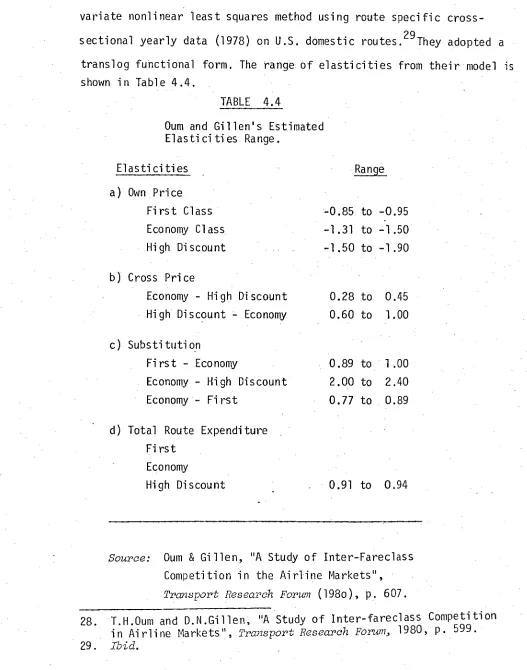
Oum and Gillen (1980) estimated the cross relationship between 26. Jud and Joseph, "International Demand for Latin American
36.
three different fare classes on the U.S. domestic trunk routes. The
three fare classes were: first class, standard economy class and
discount fare class.28 A system of demand functions for the three
fare classes were derived; they were then estimated jointly by a
multi-variate nonlinear least squares method using route specific
cross-sectional yearly data (1978) on U.S. domestic routes. 29 They adopted a
[image:41.559.24.551.150.820.2]translog functional form. The range of elasticities from their model is shown in Table 4.4.
TABLE 4.4
Oum and Gillen's Estimated Elasticities Range.
Elasticities Range
a) Own Price
First Class -4.85 to -2.95
Economy Class -1.31 to -1.50
High Discount -1.50 to -1.90
b) Cross Price
Economy - High Discount High Discount - Economy
c) Substitution
First - Economy
Economy - High Discount Economy - First
d) Total Route Expenditure First
Economy
High Discount
0.28 to 0.45 0.60 to 1.00
0.89 to 1.00 2.00 to 2.40 0.77 to 0.89
0.91 to 0.94
Source':
Oum & Gillen, "A Study of Inter-Fareclass Competition in the Airline Markets",Transport Research Forum
(198o), 10 607.28. T.H.Oum and D.N.Gillen, "A Study of Inter-fareclass Competition
in Airline Markets",
Transport Research Forum,
1980, p. 599.The own price elasticities are consistent with the belief that
first class travellers are price inelastic, while. the economy and high
discount fare class travellers are more sensitive to price. This is
because the proportion of leisure travellers is greater in the economy
and hi gh discount. fare- class .
The estimated cross elaticities show two important results: firstly,
the strong cross price elasticity of the high discount fare with
respect to the economy fare. The airlines have claimed in the past
that the high discount fare has eroded the standard economy class
market.30 The cross price elasticity estimated for the high discount
fare with respect to the economy fare suggests that if the economy fare
were reduced by 1%, between 0.6% and 1% of the-high discount travellers
would switch to travelling on economy fares. The second important
finding is that the first class fare has no significant cross
relation-ship with any other fareclass. It tends to support the practice of
separating business and leisure travellers in travel demand estimation.
The representative fare used in the model is important. Kanafani
and Sadoulet (1977) have shown that the seasonal distribution is
differ-ent for differdiffer-ent fares. For example, while the peak is the most
attractive travel season for all travellers, its relative
attractive-ness is highest for excursion travellers. 31 This indicates that
excursion fare should probably be used as the fare variable in the peak
season when modelling leisure travellers. Because of the complex
interaction in this market and their relative sensitivity to price,
the cross elasticities should be considered when developing either a
commercial or public policy aimed at pricing variation travel.
It is possible to generate a complete set of demand elasticities
30. /bid.,
p. 607.38.
for the vacation travel market from available elasticity estimates.
The missing elasticities may be inferred by constraining the demand
system to satisfy the known conditions applying to elasticities in
the system.32These conditions are:33
1) Homogeneity - in each demand equation the own price,
cross price and income elasticities sum to zero.
2) Symmetry - if Eij is the cross elasticity of demand for i
with respect to the price of j and Eji is defined similarly,
then Eij = (Rj/Ri) Eji + Rj (Ely - Eiy).
Where Rj, Ri are proportions of total expenditure, and
Eiy, Ejy are income elasticities of demand.
3) Cournot column aggregation Ri Ell = - Rj
4) Engel aggregation .t Ri Ejy = 1
By this method Taplin (1980) was able to synthesize a demand
matrix for vacation travel.34 . This is clearly not the most preferred
method to approach the problem of estimating cross elasticities,
however, given the data constraints it may be a good approximation.
S.
32. A good discussion of the known conditions applying to the . elasticities in a demand system is provided by Brown, A. and Deaton, A., "Surveys in Applied Econometrics; Models of
consumer behaviour", Economic journal, Vol .82, pp. 1145-1236.
33. J.H.E. Taplin, "A Coherence Approach to Estimates of Price
Elasticities in the Vacation Travel Market", Journal of
Transport Economics and Policy, January, 1980, p. 20.
CHAPTER 5.
MODEL SPECIFICATIONS AND DATA
The previous chapter showed the techniques and results for
various studies on airline demand. Estimation techniques have become
increasingly sophisticated and as more data has become available, the
number of explanatory variables used has increased. The literature
search revealed no previous work on estimating seasonal demand
functions. With the knowledge obtained from previous studies and the
available data a model is specified to try to capture the cross
re-lationships between travel seasons.
The main interest in this study lies in the estimation of the
cross relationships between travel seasons; there are two ways of
setting up the model. The first method is to set up a demand equation
for each travel season and estimate each season separately. 1 However,
this specification would not allow for tests of serial correlation:
as serial correlation typically occurs with the use of time series data,
it would be advisable to test for it.2 Thus the second approach is
adopted, that is to use a single equation specification. This single
equation uses dummy variables to create interaction terms which allows
variables to be switched on and off depending on the travel season.
Serial correlation leads to -estimates that are no longer efficient
and to bias in the estimation of the variance of the disturbance term.
This is a problem when using time series data because the stochastic
disturbance terms may be related to each other. A shorter time span
1. The separate equations were estimated, mainly to satisfy the
researchers that the results could be reproduced by the single equation - see Appendix B for results of separate equation.
2. M.D. Intriligator,
Economic Mbdels, Techniques and Applications
40.
between observations may alleviate the problem of identification, but
it would increase the likelihood of encountering serial correlation.
A.
SINGLE EQUATION SPECIFICATION
The general relationship for this problem may be given as:
LNT f (LNLF, LNSF, LNPF, AXUS, AXUK, Y)
(Eq. 1)
where
LNT = the number of trips per head of leisure traveller,
LNLF =, the real advanced purchase fare available in the low period,
LNSF = the real advanced purchase fare available in the shoulder period,
LNPF — the real advanced purchase fare available in the peak period,
AXUS = the U.S. to Australia relative prices,
AXUK = the U.K. to Australia relative prices,
Y = the real per capital disposable income.
This basic model will not yield any cross elasticities between travel
seasons. The travel seasons as given by the Department of Transport
for Australian residents travelling to the U.S. were:
(a) low period: February, March, October and November.
(b) shoulder period: April, 1-15 July, September, 1-15 December and January.
(c) peak period: May, June, 16-31 July, September, 1-15 December.
Because of the difficulties involved in using the split months in the
regression, it was decided to pool the split months into either a
shoulder or a peak period. To justify which months fell into which
travel season, the monthly departures from 1974 to 1980 were used to
help determine which season the split months would fit. The low period
. was kept intact, while the shoulder and peak periods are now given
(b) shoulder period: January, April, July and September.
(c) peak period: May, June, August and December.
It is known that leisure travellers are influenced by the
pub-lished fares in other travel periods. These fares and conditions are
published up to six months in advance. Thus in any one travel period,
with a little research, the potential traveller would most likely be
aware of the other fares. This influence of the other fares available
in any one travel period must be accounted for in the model. For this
purpose interaction terms/slope shifters are introduced into the model.
The generation of the interaction terms is quite simple. For instance,
to generate the shoulder fare interaction term the shoulder fare is
multiplied by the shoulder dummy variable (the shoulder dummy equals
1 for January, April, July and September, 0 otherwise). The
inter-action terms are also generated for the U.S., U.K. relative prices
and income variables.
Twelve monthly dummy variables have also been incorporated into
the model. The dummy variables pick up the seasonal effects and the
end effects. The seasonal effects are important and have been
dis-cussed. The end effects refer to the effect of a potential traveller
delaying his trip in order to take advantage of the lower fares
offer-ed at other periods. If a leisure traveller considers making his
trip towards the end of a peak month (e.g. December) he may delay his
trip till January to take advantage of the lower fares in January,
42.
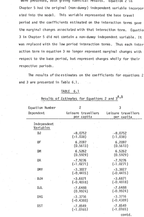
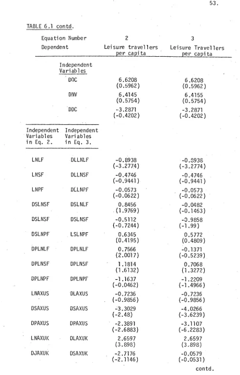
in LNT = a1 DJ + a2DF + a
3 DM + a— 4 DA + a5DMY + a6DJN + a DJL
+ a
8DAG + a9DST + a10 DPC + a11 DNV + a12 DDC.
Ln LNLF + b2 in LNSF + b3 in LNPF
+ c1 D (in LNLF) + c s 2 Ds (in LNSF) D (in LNPF)
+ c4 Dp (in LNLF) + cs Dp (in LNSF) + c6 Dp (in LNPF)
+ d
1 in AXUS
+ d2 Ds (in AXUS) + d3 Dp (in AXUS)
+ e
1
in AX
UK+ e2 Ds (Ln AXUK) + e3 D (in AXUK)
+ f1 in RDYM
+ f2 Ds (in RMYM) + f3 D (in RDYM)
+ U (Eci. 2)
where
in LNT = the log of leisure trips per capita,
DJ = dummy January = 1; 0 otherwise',
DF = dummy February = 1; 0 otherwise,
DM = dummy March = 1; 0 otherwise,
DA = dummy April = 1; 0 otherwise,
DMY = dummy May = 1; 0 otherwise,
DJN = dummy June = 1; 0 otherwise,
DJL = dummy July = 1; 0 otherwise,
DAG = dummy August = 1; 0 otherwise,
DST = dummy September= 1; 0 otherwise,
DOC = dummy October = 1; 0 otherwise,
DNV = dummy November = 1; 0 otherwise,