Coupled models of glacial isostasy and ice sheet dynamics

(1)

Coupled Models of Glacial Isostasy and Ice

Sheet Dynamics

by

Christopher Zweck, BSc(Hons)

Submitted in fulfilment of the requirements for the degree of

Doctor of Philosophy

(2)

I hereby declare that this thesis does not incorporate without acknowledgement any material previously submitted for a degree of diploma at any university. To the best of my know ledge and belief this thesis contains no material previously

published or written by another person except where due acknowledgement is made.

Christopher Zweck

This thesis may be made available for loan and limited copying in accordance with the Copyright Act 1968.

(3)

Acknowledgements

I would like to thank Garth Paltridge for excellent supervision during the course of this work. Thanks also go to Roland Warner and Bill Budd for their encour-agement and support. Many thanks also to Richard Coleman for the OSU91A satellite data and extraction code.

(4)

Abstract

This thesis deals with the incorporation of isostatic processes into realistic mod-els of ice sheet dynamics. A viscoelastic half-space model of isostatic adjustment is developed, and as an initial exercise is coupled to a model of the Antarctic ice sheet simulating the last glacial cycle. The ice sheet model is a three-dimensional, time-dependent model originally formulated by Jenssen (1977) where the driving input data are net accumulation of snow and eustatic sea level change. This allows examination of the sensitivity of the ice sheet sim-ulation to changes in the parameters of the isostatic model. In general, the maximum ice volume generated over a glacial cycle decreases with increasing mantle viscosity and increasing lithospheric rigidity.

To obtain realistic values for the isostatic parameters of mantle viscosity and lithospheric rigidity the retreat of the Northern Hemisphere ice sheets and the subsequent isostatic adjustment since the last ice age is simulated. The isostatic parameters are adjusted until the overall model provides the best match to relative sea level data, with the eustatic component of the relative sea level change prescribed. (The maximum value of the amplitude of the prescribed sea level change is 130 m as determined from the Huon Peninsula in Papua New Guinea). Initially the simulation and matching procedure is performed using a simple ice sheet model whose time dependent extent is set by the ICE4G dataset (Peltier, 1994) and whose thickness and volume is set on the assumption of a parabolic profile of thickness. From these trials the model parameters that most realistically reproduce the observed isostatic adjustment associated with the retreat of the Laurentide ice sheet are 3 x 1021 Pa s for lower mantle viscosity, 2 x 1021 Pa s for upper mantle viscosity and 1 x 1025 N m for lithospheric rigidity. For the Fennoscandian ice sheet the corresponding parameter values are 6 x 1021 Pa s, 4 x 1021 Pa s and 6 x 1024 N m. The trials are then repeated with the parabolic profile ice sheet assumption replaced by generation of ice sheet thickness using the Jenssen ice sheet model. For the Laurentide ice sheet the same earth model parameters are recovered. For the Fennoscandian ice sheet the use of the Jenssen model to simulate ice thickness produces earth model parameters of 1.3 x 1021 Pas for both the lower and upper mantle viscosity and

(5)

iv

2 x 1025 N m for the lithospheric rigidity. A problem with the analysis is that the maximum volume of the combined ice sheets corresponds only to 50 m of eustatic sea level change in the case of the parabolic profile simulation and to 40 m when using the Jenssen model.

The sensitivity of the Antarctic ice sheet to regional variations in litho-spheric rigidity is examined. Using a range of simple relations between crustal thickness (for which there exists data on geographic distribution) and spheric thickness, it is determined that the main effect of non-uniform litho-spheric thickness is on the extent of the Ronne and Amery ice shelves.

The constraint of prescribed eustatic sea level change since the last ice age is removed by linking the Laurentide, Fennoscandian and Antarctic ice sheet models via the common sea level change determined by the deglaciation of the combined ice sheets. The constraint on Northern Hemisphere ice sheet extent is also removed by allowing the ice sheet model (the Jenssen model) t<;> determine its own extent when driven by climatology and the Milankovitch cycles of solar input. This overall model produces a realistic eustatic sea level change since the last ice age (130 m), but unrealistic changes in relative sea level. In some locations the calculated relative sea level changes are too large by 200 m.

(6)

...

9. Conclusions

Bibliography .

10. Appendix A .

11. Appendix B .

vii

. 129 . 129 . 133 . 134 . 134 . 134 . 137 . 138 . 141 . 144

. 148

. 155

. 164

(9)

LIST OF TABLES

3.1 Values of asthenospheric diffusivity used in various ice sheet models.

5.1 Best fit earth model parameters using parabolic profile approxi-mation to generate deglaciation chronology. . . . 5.2 Best fit earth model parameters using time-dependent ice sheet

model to generate deglaciation chronology. . . .

6.1 Best fit earth model parameters using parabolic profile approxi-mation to generate deglaciation chronology.

...

6.2 Best fit earth model parameters using time-dependent ice sheet

model to generate deglaciation chronology. . . .

7.1 Minimum, maximum and average values of the effective elastic thickness (km) and lithospheric rigidity (Nm) used in the case of direct proportionality between the crust and lithosphere. . . . 7.2 Minimum, maximum and average values of the effective elastic

thickness (km) and lithospheric rigidity (N m) used when the lithospheric thickness is equal to the crustal thickness plus a constant.

22

69

81

95

104

118

122

8.1 Latitude dependent elevation of the 1 m yr-1 ablation rate. 132

(10)

List of Tables

9.2 Earth model parameters, fit to relative sea level data and pre-diction, of present day sea level change for North American and Northern European adjustment . . . .

9.3 Deviation in total ice sheet volume from the standard earth model (5) for different earth models and earth model

parame-ix

150

(11)

LIST OF FIGURES

2.1 Latitude dependence of snow line elevation and corresponding ice sheet accumulation/ablation. . . 12

3.1 Antarctic ice sheet thickness (km) at the present day. . . 18 3.2 Equilibrium Antarctic lithospheric deflection (km) corresponding

to the ice load of the present day. . . 19 3.3 Steady state deformation of a parabolic profile ice sheet for

var-ious lithospheric rigidities. Solid lines represent the Fourier so-lution and symbols represent the Hankel soso-lution. Archimedean displacement ratio is the deflection profile divided by the ratios of density of ice and the earth's mantle. . . 25 3.4 Surface profile of earth for instantaneous unloading and thin

channel flow at 1, 5 and 10 kyr after unloading. Solid lines rep-resent the Fourier solutions and symbols reprep-resent the Hankel solutions. Archimedean displacement ratio is the deflection pro-file divided by the ratios of density of ice and the earth's mantle. 28 3.5 Surface profile of earth for instantaneous unloading and

half-space flow at 1,5 and 10 kyr after unloading. Solid lines represent the Fourier solution and symbols represent the Hankel solution. Archimedean displacement ratio is the deflection profile divided by the ratios of density of ice and the earth's mantle. . . 28 3.6 Surface profile of earth for instantaneous loading and half-space

(12)

List of Figures

3. 7 Surface profile of earth for instantaneous unloading and half-space flow at 1,5 and 10 kyr after unloading. Solid lines represent the decoupled viscoelastic (Fourier) solution and symbols repre-sent the Maxwellian viscoelastic (Hankel) solution. Archimedean displacement ratio is the deflection profile divided by the ratios

xi

of density of ice and the earth's mantle. . . 31

4.1 Variation in sea level (Chappell and Shackleton, 1986). 35 4.2 Variation in surface accumulation (Jouzel et al, 1987). . 35 4.3 Ice sheet elevation (km) of Antarctica defined as the equilibrium

state. . . 37 4.4 Bedrock topography (km) of Antarctica defined as the

equilib-rium state. . . 37 4.5 Time-dependent change in the total volume of ice on Antarctica

for the 'no isostasy' model, the 'instantaneous isostasy' model and the standard earth model. . . 38 4.6 Predicted surface elevation (km) of Antarctica at present day

after the 160 kyr run of the standard earth model. . . 40 4. 7 Predicted surface elevation (km) of Antarctica at present day

after the 160 kyr run of the 'no isostasy' model. . . 40 4.8 Difference in bedrock elevation (km) at the present day between

the standard earth model and the 'no isostasy' model. . . 41 4.9 Time-dependent change in the total volume of ice for the

stan-dard earth model, the thin channel model and the 'instantaneous adjustment' model. . . 42 4.10 Decay time as a function of wavenumber for the thin channel and

standard earth models. Huybrechts' decay time for Antarctica (referred to in Chapter 3) is circled. The histogram represents the wavenumber range for the ice thickness distribution of the Antarctic ice sheet considered in this study. . . 43 4.11 Locations in Antarctica where model predictions of isostatic

(13)

List of Figures

4.12 Model predicted isostatic adjustment for the last 15 kyr BP at selected locations. Solid line represents the standard earth model

xii

and dashed line represents the thin channel model. . . 44 4.13 Time-dependent change in the total volume of ice for the

stan-dard earth model (1021 Pas), the 1020 Pas viscosity model and the 1022 _{Pa s viscosity model. . . 46}

4.14 Model predicted isostatic adjustment for the last 15 kyr BP at selected Antarctic locations. Solid line represents the standard earth model (1021 _{Pas), dot-dashed line represents the 10}20 _Pas

viscosity model and dashed line represents the 1022 Pa s viscosity model. . . 47 4.15 Difference in ice sheet elevation (km) at 20 kyr BP between

stan-dard earth model and 1022 Pa s viscosity model. . . 48 4.16 Difference in ice sheet elevation (km) at the present day between

standard earth model and 1022 Pa s viscosity model. . . 48 4.17 Time-dependent change in the total volume of ice for the

stan-dard earth model (lithospheric rigidity equal to 1025 Nm), the 1024 _{N m rigidity model and the 10}26 _{N m rigidity model. . . 49}

4.18 Predicted difference in ice sheet thickness (km) at the present day between the 1026 N m rigidity model and the 1024 N m rigidity model. . . 50 4.19 Predicted difference in bedrock elevation (km) at the present day

between 1026 N m rigidity model and 1024 N m rigidity model. 50 4.20 Model predicted isostatic response for a last 15 kyr BP at

(14)

List of Figures

4.22 Time-dependent change in the total volume of ice for the stan-dard earth model (0%), the 15% gravity anomaly model and the 30% gravity anomaly model. For all models the standard earth model parameter values (1021 Pas viscosity and 1025 N m

rigid-xiii

ity) are used. . . 56

5.1 Model domain and relative sea level data locations for the Lau-rentide ice sheet. Large circles indicate sites where data have

been wholly excluded. . . 58

5.2 ICE4G ice extent at 20 kyr BP. . 59

5.3 ICE4G ice extent at 10 kyr BP. . 59

5.4 ICE4G ice extent at the present day. 59

5.5 Parabolic profile ice sheet thickness at maximum extent (21 kyr BP). 61 5.6 Observed and predicted relative sea level heights for 'best fit'

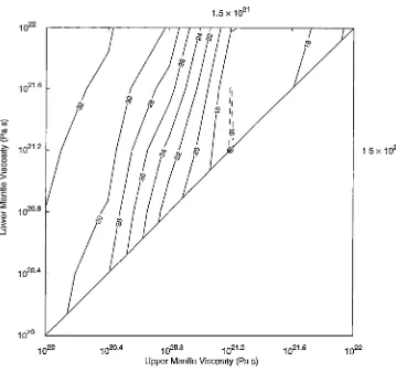
earth model parameter values using the Lambeck (1993c) defini-tion of variance. . . 64 5.7 Parameter space for 3 layer earth model with upper mantle and

lower mantle viscosities as searching parameters. The minimum in parameter space is shown by EEl with corresponding earth model parameter values shown in exponential notation at top and right hand side of axes. Note that from pressure arguments the viscosity of the lower mantle must be greater than the vis-cosity of the upper mantle and hence there are no contours to the right of the diagonal line of equal viscosities. . . 66 5.8 Variance as a function of ice sheet rescaling factor

f3

for uniform

mantle viscosity of 1.5 x 1021 Pa s and lithospheric rigidity of 1025 N m. Minimum variance occurs for

f3

= 0.9. . . 67 5.9 Parameter space for 3 layer earth model with upper mantle

(15)

List of Figures

5.10 Parameter space for 3 layer earth model with upper and lower mantle viscosities as searching parameters. The minimum in pa-rameter space is shown by EB with corresponding earth model parameter values shown in exponential notation at top and right hand side of axes. Note that from pressure arguments the vis-cosity of the lower mantle must be greater than the visvis-cosity of the upper mantle and hence there are no contours to the right of

xiv

the diagonal line of equal viscosities. . . 70 5.11 Parameter space for 3 layer earth model with upper mantle

vis-cosity and lithospheric rigidity as searching parameters. The minimum in parameter space is shown by EB with corresponding earth model parameter values shown in exponential notation at top and right hand side of axes. . . 71 5.12 Observed and predicted relative sea level heights for best fit earth

model. Underestimation at James Bay for RSLobs = -250 m is circled. . . 73 5.13 Frequency distribution of misfit between modelled and observed

relative sea level data. To the right of 0 corresponds to underes-timation and to the left of 0 corresponds to overesunderes-timation. . . . 73 5.14 Geographic distribution of error between observed and predicted

sea level heights at individual sea level locations. . . 74 5.15 Annual precipitation (m yr-1) over North America (Shea, 1986). 76 5.16 Annual mean temperature (°C) over North America (Shea, 1986). 76 5.17 Ice sheet thickness (km) at 21 kyr BP generated as a first

approx-imation using the time-dependent ice sheet model and ICE4G chronology of ice extent . . . 78 5.18 Parameter space for an earth model with uniform mantle

(16)

List of Figures

5.19 Parameter space for an earth model with uniform mantle vis-cosity and lithospheric rigidity as searching parameters. The minimum in parameter space is shown by E9 with corresponding earth model parameter values shown in exponential notation at

xv

top and right hand side of axes. . . 80 5.20 Parameter space for 3 layer earth model with upper and lower

mantle viscosity as searching parameters. The minimum in pa-rameter space is shown by E9 with corresponding earth model parameter values shown in exponential notation at top and right hand side of axes. Note that from pressure arguments the vis-cosity of the lower mantle must be greater than the visvis-cosity of the upper mantle and hence there are no contours to the right of the diagonal line of equal viscosities. . . 82 5.21 Parameter space for 3 layer earth model with upper mantle

vis-cosity and lithospheric rigidity as searching parameters. The minimum in parameter space is shown by E9 with corresponding earth model parameter values shown in exponential notation at top and right hand side of axes. . . 83 5.22 Parameter space for 3 layer earth model with upper mantle

vis-cosity and f3 searching parameters. The minimum in parameter space is shown by E9 with corresponding earth model parameter value shown in exponential notation at top of axes. . . 85 5.23 Observed and predicted relative sea level heights for best fit earth

model. . . 86 5.24 Frequency distribution of misfit between modelled and observed

sea level heights at individual sea level locations. . . 87 5.26 Equivalent eustatic sea level contribution of both ice sheet

(17)

List of Figures xvi

5.27 Present day uplift rate (mm yr-1) calculated using parabolic

profile ice sheet model. . . 89 5.28 Present day uplift rate (mm yr-1) calculated using time-dependent

ice sheet model. . . . 5.29 Location of present day tide gauge stations.

5.30 Observed sea level change and model predicted adjustment veloc-89 90

ity for ice sheet model generated deglaciation chronology (r=0.8382) and parabolic profile ice sheet chronology (r=0.8276). . . 91

6.1 Model domain and relative sea level data locations for the Fennoscan-dian ice sheet. Large circles indicate sites where data have been

wholly excluded.

...

6.2 Parabolic profile ice sheet reconstruction at maximum extent (21 kyr BP) derived from ICE4G . . . 6.3 Least Squares Variance solution space for 3 layer earth model

with upper mantle and lower mantle viscosities as searching pa-rameters. The minimum in parameter space is shown by EB with corresponding earth model parameter values shown in exponen-tial notation at top and right hand side of axes. Note that from pressure arguments the viscosity of the lower mantle must be greater than the viscosity of the upper mantle and hence there are no contours to the right of the diagonal line of equal viscosities. 6.4 Least Squares Variance solution space for 3 layer earth model

with upper mantle viscosity and lithospheric rigidity as search-ing parameters. The minimum in parameter space is shown by

93

95

96

EB with corresponding earth model parameter values shown in exponential notation at top and right hand side of axes. . . 97 6.5 Observed and predicted relative sea level heights for best fit earth

model using parabolic profile ice sheet deglaciation chronology. . 98 6.6 Geographic distribution of error between observed and predicted

(18)

List of Figures xv ii

6.8 Annual mean temperature (°C) over Northern Europe (Shea, 1986).101 6.9 Parameter space for 3 layer earth model with upper mantle and

lower mantle viscosities as searching parameters. The minimum in parameter space is shown by EB with corresponding earth model parameter values shown in exponential notation at top and right hand side of axes. Note that from pressure arguments the viscosity of the lower mantle must be greater than the vis-cosity of the upper mantle and hence there are no contours to the right of the diagonal line of equal viscosities. . . 102 6.10 Parameter space for 3 layer earth model with upper mantle

vis-cosity and lithospheric rigidity as searching parameters. The minimum in parameter space is shown by EB with corresponding earth model parameter values shown in exponential notation at top and right hand side of axes . . . 103 6.11 Observed and predicted relative sea level heights for best fit

earth model using time-dependent ice sheet model deglaciation chronology. . . 105 6.12 Frequency distribution of misfit between modelled and observed

sea level heights at individual sea level locations. . . 106 6.14 Parameter space for 2 layer earth model with (3 and uniform

mantle viscosity as searching parameters. The minimum in pa-rameter space is shown by EB with corresponding earth model parameter value shown in exponential notation at top of axes. . . 107 6.15 Present day uplift rate (mm yr-1) for parabolic profile ice sheet

model. . . . 109 6.16 Present day uplift rate (mm yr-1) for time-dependent ice sheet

model. . . . . 6.17 Location of present day tide gauge stations.

(19)

List of Figures xvi ii

6.18 Observed sea level change and model predicted adjustment veloc-ity for ice sheet model generated deglaciation chronology (r=0.9278) and parabolic profile ice sheet chronology (r=0.9180). . . . . 110

7.1 Cratonic structure of Antarctica. EA=East Antarctica, E= Ellsworth Block, P=Antarctic Peninsula, T=Thurston Block, B=Marie Byrd Land Block. . . . 113 7.2 Equilibrium deflection (km) calculated for Antarctic ice sheet

using finite difference sparse matrix methods . . . 116 7.3 Crustal thickness (km) of Antarctica (Demenitskaya and Ushakov,

1966) . . . 117 7.4 Time-dependent change in the total volume of ice for the

stan-dard earth model, the 'crust x 2' model, the 'crust x 3' model and the 'crust x 4' model. . . 120 7.5 Difference in ice sheet thickness (m) between the 'crust x 4'

model and the standard earth model at 80 kyr BP. . . 121 7.6 Grounding lines for the 'crust x 4' model (thin line) and the

standard earth model (thick line) at 80 kyr BP . . . 121 7. 7 Time-dependent change in the total volume of ice for the

stan-dard earth model, the 'crust

+

30 km' model, the 'crust + 50 km' model and the 'crust + 70 km' model. . . . 123 7.8 Difference in ice sheet thickness (m) between the 'crust+ 30 km'

model and standard earth model at 80 kyr BP. . . 124 7.9 Grounding lines for the 'crust + 30 km' model (thin line) and

the standard earth model (thick line) at 80 kyr BP. . . . . 124 7.10 Equilibrium deflection for a parabolic profile ice sheet for

differ-ing but uniform lithospheric rigidities. . . 125 7.11 Figure A shows the thickness distribution for each lithosphere

(20)

List of Figures

7.12 Bedrock topography, ice shelf thickness and ice shelf elevation as a function of time for a cross section through the Ronne ice shelf. The continental shelf is the dark shading and the ice shelf is the

xix

light shading . . . 128

8.1 Summer solar insolation difference (W m-2) from the present

day as a function of time (160 kyr BP to the present) and latitude.131 8.2 Time-dependent change in 'above :floating' ice volume as an

equiv-alent eustatic sea level contribution for the Laurentide, Fennoscan-dian and Antarctic ice sheets with the

/3

values of Budd and Smith (1981) . . . 135 8.3 Time-dependent change in 'above :floating' ice volume as an

equiv-alent eustatic sea level contribution for the Laurentide, Fennoscan-dian and Antarctic ice sheets with

/32

= 6.8° for the Laurentide ice sheet and

/32

= 6.4° for the Fennoscandian ice sheet. . . . . . 136 8.4 Model predicted change in global eustatic sea level over the last

glacial cycle using new values of

/32.

Also shown are the global eustatic sea level curve of Chappell and Shackleton (1986) and the SPECMAP eustatic sea level curve (Martinson et al, 1987) . . 137 8.5 Model prediction of Laurentide ice sheet elevation at 21 kyr BP. 139 8.6 Model prediction of Fennoscandian ice sheet elevation at 21 kyr BP .139 8.7 Free air gravity anomaly (mgal) over North America from

Wal-cott (1970) . . . 140 8.8 Observed and predicted relative sea level heights for both the

Laurentide and Fennoscandian isostatic adjustment. . . . . 141 8.9 Geographic distribution of error between observed and predicted

sea level heights at individual sea level locations for the Lauren-tide ice sheet . . . 143 8.10 Geographic distribution of error between observed and predicted

(21)

List of Figures

8.11 Model prediction of isostatic adjustment at Churchill since the last ice age. Dot-dashed line is prediction from 'best fit' deglacia-tion chronology for the Laurentide ice sheet in Chapter 5. Solid line is the prediction of adjustment for the climatological model used in this chapter. . . .

9.1 Elevation of Laurentide ice sheet at maximum extent.

xx

145

(22)

1.

INTRODUCTION

The retreat of the ice sheets at the end of the last ice age is arguably the most profound change to the surface of the earth in recent geological time. This transformation is a key focus of inquiry for two distinct fields of research. On the one hand the isostatic adjustment following the ice retreat is one of a limited set of phenomena that allow investigation of the properties of the deeper earth. On the other hand the behaviour of the ice in response to the climate change which drove the retreat allows the development of an understanding of the behaviour of present day ice sheets.

Naturally the choice of which ice sheet to study in these fields is determined by the availability of data. The glacio-geomorphology and isostatic adjustment of former ice sheets such as the Laurentide and Fennoscandian are well un-derstood, but their thickness and elevation at the last glacial maximum are debatable. For these reasons they are examined more in isostatic modelling than in ice sheet modelling. For ice sheets such as Antarctica and Greenland the present day ice sheet thickness and elevation are well constrained, but the extent and isostatic adjustment of these ice sheets at the last glacial maximum are not. For these reasons they are examined more closely in ice sheet modelling than in isostatic modelling.

The study of ice sheets and the study of glacial isostasy have emerged from separate disciplines. As a result of this separation it is not surprising that in each discipline assumptions regarding the other are invoked. Peltier (1996b) states:

(23)

1. Introduction

history. Similarly, recently proposed models of the deglaciation history may be sensitive to errors in the model of the radial variation of viscosity.

2

Several authors have examined this sensitivity and suggested that the conclu-sions generated from isostatic models are sensitive to the form of the ice sheet assumed in the calculation (Han & Wahr, 1995; Fang & Hager, 1996). Ice sheet modelling results show a sensitivity to assumptions about how isostasy is implemented (Le Meur & Huybrechts, 1996; Lingle & Clark, 1985).

(24)

2. LITERATURE REVIEW

This section reviews the physical interactions between isostasy and ice sheets. It is divided into three sections. The first reviews the treatment of isostasy in ice sheet models. The second reviews the treatment of ice sheets in models of isostasy. The last section reviews the results of coupled earth/ice-sheet models.

In much of this thesis there is reference to eustatic and relative sea level change. It should be explained that in the present study eustatic sea level change is the change in sea level elevation which results from changes in ocean volume with time. In the present study the change in ocean volume is assumed to reflect changes resulting from the growth and retreat of ice sheets. Relative sea level indicates changes in ocean surface area with respect to the present day surface profile of the earth. Thus relative sea level changes account for both the isostatic adjustment of the earth and the eustatic sea level change of the ocean.

2.1 The Treatment of Glacial Isostasy in Ice Sheet Models

(25)

2. Literature Review 4

larger than the geological evidence suggested. Takeuchi (1963) reintroduced the thin channel model with the justification that it predicted more realistic isostatic adjustment rates than the half-space model (Peltier, 1980). Coupled with a model of lithospheric adjustment introduced by McConnell (1965) the thin channel model has been adopted as an adequate representation of glacial isostasy for ice sheet modelling by authors such as Huybrechts (1992) and Le-treguilly and Ritz (1993).

The thin channel model predicts submergence peripheral to the Northern Hemisphere ice sheets during their retreat (Officer et al., 1988). Peripheral submergence following ice sheet retreat has been documentedc in the geolog-ical record (Livermann, 1994), but McConnell (1965) realised that this be-haviour is also produced by a half-space earth model with viscosity that in-creases radially towards the earth's core. Investigations subsequent to those of McConnell have incorporated viscosity stratifications as a function of depth to explain the peripheral submergence, with authors such as Fjeldskar and Cathles (1991) invoking the notion of a 'low viscosity channel' beneath the lithosphere which produces similar behaviour to the thin channel flow model. Sigmundsson (1991) suggested that the existence of a low viscosity channel with viscosity 1 x 1019 Pa s can explain the relative sea level data for Iceland. Sigmundsson noted however that this result could reflect a lateral variation in viscosity, as Iceland is located directly over a mid-oceanic ridge. Breuer and Wolf (1995) suggest that a channel with viscosity in the range 3 x 1018 Pa s to 2 x 1019 Pa s can explain the adjustment in the Svalbard Archipelago. However Mitrovica (1996) notes that varied estimates of mantle viscosity have been made for the Svalbard Archipelago, and attributes this variation to the limited knowledge of the ice sheet history over the region. Lambeck et al (1996) suggest that for the British Isles it is necessary to invoke a low viscosity channel if the thickness of the lithosphere is assumed to be less than 50 km. A lithospheric thickness of less than 50 km was also found to be consistent with the low viscosity channel concept of Fjeldskar and Cathles.

(26)

denying the existence of a rigid substratum beneath a low viscosity channel on the basis of seismic evidence. Certainly the use of the thin channel assumption can greatly influence the modelled behaviour of the ice sheet itself. Letreguilly and Ritz (1993) concluded that, when using the thin channel adjustment model in an ice sheet model, an advancing ice sheet produces an isostatic forebulge a few hundred metres high so that the shallow sea floor to the front of the sheet is raised above sea level and is subsequently covered by the ice. The forebulge results from an excess of mantle material at the edge of the ice sheet that has been 'squeezed out' from beneath the ice to accommodate the isostatic adjustment. For a half-space model the induced flow in the earth's mantle is predominantly vertical and a forebulge of a few hundred metres is not possible. This would in turn suggest that the shallow sea floor to the periphery of the ice sheet is not raised above sea level and is not covered by ice. The advance of the ice sheet is therefore overestimated by the use of the thin channel flow model.

The bias of the thin channel flow model towards a greater ice advance dur-ing a period of growth has also been reported by Marsiat (1994). In her study a larger magnitude of advance and retreat for the ice sheet occurs when using a thin channel earth model than when using a simple physically-parametrised iso-static adjustment model. For reasons similar to those suggested by Letreguilly and Ritz, Marsiat concluded that the forebulge created around the ice sheet by the thin channel flow model allows the ice to advance further over the sur-face of the continent. Her results showed that 38% more ice is generated over a glacial cycle when using the thin channel flow model than when using the parametrised adjustment model, corresponding to a maximum difference in the generated eustatic sea level change of 36 m.

(27)

West Antarctic Peninsula is accelerated by an increase in the viscosity of the thin channel model. This result is not consistent with the suggestion of Oerle-mans and Van der Veen. Payne et al concluded that the reduction in the rate of isostatic adjustment increases the rate of ice sheet decay by calving. With the increase in sea level the ice sheet is in contact with the ocean for longer and experiences higher calving rates.

The discussion above has concerned the potential sensitivity of an ice sheet model to the treatment of isostasy. The following section concerns the reverse situation - namely the sensitivity of models of isostasy and of deduced isostatic parameter values to the treatment and history of ice sheets.

2.2 The Reconstruction of Ice Sheets for Isostatic Models

Sophisticated geophysical models of isostasy such as those derived by Peltier (1989) and Lambeck (1987) envisage a viscoelastic mantle rheology and a spheri-cal self-gravitating earth to deduce the viscosity stratification of the inner earth. However, as the forcing for these earth models involves the history of ice sheet deglaciation, the issue of the influence of assumptions about the ice sheet is very important.

(28)

best predicted the relative sea level, Wu and Peltier assumed that the residual error was due to the inaccuracies in the deglaciation chronology. This assump-tion was based on the argument that near the centre of the former ice sheets the isostatic adjustment can be separated into an adjustment-amplitude (that depends on the ice sheet thickness) and an adjustment-rate (that depends on the mantle viscosity). They claimed that the ice sheet history and isostatic adjustment can be decoupled so that the ice sheet deglaciation chronology can be modified to produce an improvement in the prediction of the relative sea level data. Using ICEl, the modification process first attempts to deduce the best mantle viscosity profile which fits the relative sea level and free air gravity anomaly data. The gravity data was used as an indication of the present day state of isostatic disequilibrium in formerly glaciated regions (Walcott, 1970). When the viscosity profile that most realistically reproduced the observations was found the ice sheet thicknesses and extents were manually adjusted (thus creating the ICE2 chronology) until the sea level and gravity data was recon-ciled. With ICE2 Wu and Peltier found that although the model prediction of relative sea level data close to the ice sheets matched the observations bet-ter than when using ICEl, the relative sea level data far from the ice sheet (in New Zealand and Brazil) showed an anomaly of 2 kyr in response time. This anomaly in the far field data was attributed to the lack of consideration of the eustatic sea level contribution from other ice sheets such as Antarctica. Peltier (1988) found that by adding a delayed Antarctic deglaciation and by using a thick lithosphere in his model, the far field relative sea level data could be reconciled with the ICE2 chronology. However Nakada and Lambeck (1987) used a global spherical harmonic model to show the far field relative sea level calculations were sensitive to the finite element methodology used by Peltier. Nakada and Lambeck were able to reconcile the far field relative sea level data without using a thick lithosphere model.

(29)

most responsible for 30% of the observed free air gravity anomaly over formerly glaciated regions. James proposed that the residual anomaly is caused by ef-fects such as mantle convection. Le Meur (1996) concluded that for an isostatic model of adjustment over Northern Europe it is difficult to reconcile present day free air gravity data with present day radial velocity data.

The procedure used by Tushingham and Peltier to derive ICE3G was to infer earth model parameters and adjust the ice sheet thicknesses so that the agreement with the near field relative sea level data was as close as possible. Then both the near and far field relative sea level data was used to test the realism of the deglaciation chronology (Tushingham & Peltier, 1991). Nineteen iterations between earth model parameters and ice sheet thicknesses were used in deriving ICE3G. The corrections were made manually at every iteration to the ice sheet thicknesses and the ice sheet extent. The fit at some near field sites was still not complete. In North America between Nova Scotia and Cape Cod the fit to some sites was within experimental error while at other sites it was not. Tushingham and Peltier suggested that the ice sheet model resolution was too low to fully reproduce the deglaciation process.

To test the accuracy of ICE3G Tushingham and Peltier (1991) compared the model-generated changes in eustatic sea level to those calculated on the basis of

01

8₀_{and coral reef data. In the Huon Peninsula in Papua New Guinea}

the observed eustatic sea level rise was 130 m since the last glacial maximum (Chappell & Shackleton, 1986), whereas ICE3G suggested 115 m and ICE2 sug-gested 97 m. The Northern Hemisphere ice sheets represented in ICE3G were thinner than in ICE2 but ICE3G included an Antarctic deglaciation chronology with volume change equivalent to a eustatic sea level contribution of 26 m.

(30)

Fang and Hager (1996) used a continuous radially-dependent viscosity model (as opposed to the stratified viscosity model of Tushingham and Peltier) to compare relative sea level predictions from ICEl combined with the Antarctic deglaciation chronology of Nakada and Lambeck (1987) with those generated from ICE3G. Fang and Hager concluded that ICEl has a better overall fit to the relative sea level data than ICE3G, suggesting that the iterative process used to generate ICE3G has to some extent been biased by the stratified viscosity assumption.

Relative sea level data is used to generate ICE3G and its accuracy is there-fore dependent on the spatial distribution of the data. Following the publica-tion of addipublica-tional relative sea level data, Peltier (1994) developed the ICE4G deglaciation chronology using ICE3G as an initial estimate and iteratively mod-ifying the earth model and ice sheet deglaciation chronology three times. In this chronology Peltier also introduced a time-dependent shoreline migration which Johnson (1993) argued is important in the calculation of relative sea level. The calculation of eustatic sea level change using ICE4G shows an ex-cellent correspondence to that observed at New Guinea and Barbados (Peltier, 1994).

The ICE series is the only deglaciation chronology where the ice sheet thick-nesses are modified iteratively to reconcile the relative sea level data. Lambeck

(31)

thick-2. Literature Review 10

nesses and earth model parameters. Another advantage of a parameter space search is that an estimate can be made of the sensitivity of the earth model and ice sheet deglaciation chronology to the parameters themselves (Lambeck, 1993c). For example a reduced lithospheric rigidity in the model allows a thin-ner ice sheet to satisfy the relative sea level data (Lambeck et al., 1996). The trade-off between ice sheet thickness and lithospheric rigidity occurs because a thin lithosphere allows a greater deflection and a thinner ice sheet is required to produce the correct isostatic deflection.

(32)

2.3 Coupled Earth/Ice-Sheet Models

Oerlemans and Van der Veen's (1984) primary thesis on the effect of glacial isostasy on the behaviour of ice sheets is that isostasy accelerates both the advance and retreat of ice sheets over a glacial cycle. This property was pro-posed as an important non-linear mechanism in the accurate simulation of the growth and decay of ice sheets in response to orbitally induced radiation changes (Pollard, 1978). The Milankovitch theory of ice ages suggests that ice sheet behaviour is dominated by changes in incident radiation associated with the earth's cyclical orbital variations of period 21, 23 and 41 kyr. However the global change in ice volume reflected as a global eustatic sea level change (see Figure 4.1 for Chappell and Shackleton, 1986) is distinctly sawtoothed in form with an overall 90 kyr advance and 10 kyr retreat over a glacial cycle. It has been suggested that glacial isostasy modulates the ice sheet behaviour so that the cyclic orbital radiation changes produce the observed sawtooth pattern of advance and retreat (Pollard, 1982). This possible modulation of the ice sheet behaviour generated early interest in the coupling of ice sheet and isostatic models.

(33)

North Snow Line

Arctic Ocean

Accumulation

Northern Hemisphere Ice Sheet

Ablation

Fig. 2.1: Latitude dependence of snow line elevation and corresponding ice sheet accu-mulation/ ablation.

characteristic of the Pleistocene era. Furthermore the asthenospheric diffusivity and density were considered as separate parameters in the model formulation. In reality the diffusivity is a function of density. The combinations of diffusivity and density for which self-sustained oscillations do occur in the model are not realistic.

(34)

a reduced magnitude of growth and decay of the ice sheet, and attributed the reduction to the inclusion of the lithosphere. However the reasons why ice sheet growth and decay is exaggerated using a thin channel flow model compared to a half-space model were outlined previously in this chapter. This exaggera-tion explains why Pollard reported increased ice sheet volume changes using a thin channel flow model compared to Oerlemans and Birchfield et al (who used a physically-parametrised isostatic adjustment model) and Birchfield and Grumbine (who used a half-space adjustment model). Le Meur and Huybrechts (1996) noted that the prediction of isostatic adjustment is similar between a localised isostatic adjustment model and a viscoelastic half-space adjustment model.

(35)

the decay time increases towards the 30 kyr value used by Oerlemans. With the long decay time the isostatic adjustment rate is reduced and the ice sheet can remain longer in a region of net ablation so that a significant amount of ice is lost. In a half-space model the decay time is inversely proportional to the spatial scale of the ice sheet (Cathles, 1975). For this model at maximum extent the isostatic adjustment is fast so that the ice sheet quickly responds to the increased ablation by rising above the snow line, thereby reducing the magnitude of ice volume change. De Blonde and Peltier suggested that the conclusion of Oerlemans and Van der Veen (1984) that isostasy enhances the advance and retreat of ice sheets is only valid when using the thin channel flow approximation.

There are two papers of particular relevance to the present study. Lingle and Clark (1985) coupled a one dimensional model of an ice stream to a three dimensional viscoelastic half-space isostatic model to study the sensitivity of the modelled ice stream 'E' in West Antarctica to several different isostatic schemes. They concluded that the response of the earth to a thinning ice stream serves to delay the retreat of the ice stream grounding line. This is because ice sheet calving caused by an increase in eustatic sea level (associated with deglaciation of the Northern Hemisphere ice sheets) is counteracted by the isostatic uplift of the earth beneath the ice stream. In a model without isostasy the ice stream is flooded allowing a faster rate of ice sheet calving and grounding line retreat. This result of Lingle and Clark (1985) agrees with that of Payne et al (1989) who used a thin channel flow model in association with a model of the West Antarctic Peninsula ice sheet. These combined results suggest that this behaviour is not limited to the thin channel flow model.

(36)

(37)

3. THE EARTH MODEL

This section outlines the manner in which the isostatic adjustment of the earth is represented in the present study. A limited-area flat-earth model domain is used so as to be consistent with the ice sheet model.

The neglect of the earth's sphericity can be important. Wolf (1984) suggests that for ice sheets the size of the Laurentide the neglect of the curvature of the earth underestimates the isostatic adjustment at the ice sheet edge by up to 40% compared to spherical models. Also changes in relative sea level can only be computed to first-order as globally consistent gravitational hydro-eustatic loading cannot be calculated. The first-order representation of the relative sea level equation defines change in relative sea level as the sum of glacio-isostatic adjustment, hydro-isostatic adjustment and spatially uniform (not gravitation-ally consistent) hydro-eustatic change.

Amelung and Wolf (1994) suggest that a flat earth model is preferable to a global spherical model that does not incorporate gravitational self consistency in the relative sea level equation. They also argue that global models which do not consider the gravitational anomaly associated with the change in surface shape of the earth (incremental gravitational force) are less realistic than flat earth models which ignore this feature. Thus the error in assuming a flat earth model tends to be cancelled by the fact that it does not treat changes in the force of gravity associated with changes in the surface shape and loading of the earth.

(38)

3. The Earth Model 17

3.1 The Lithosphere

Barrel (1914) introduced the term 'lithosphere' to represent the strong outer layer of the earth under which the more viscous mantle flowed to maintain isostatic compensation. The differential equation governing the ultimate

re-gional equilibrium deflection of the lithosphere resulting from the application of a surface load is (Brotchie & Silvester, 1969)

(3.1)

where c.p is the deflection of the lithosphere due to the application of the load, Pm is the mantle density, g is the acceleration due to gravity and

Q

is the applied load.

Q

can represent either the glacio- or hydro-isostatic loading

glacio-isostasy

hydro-isostasy

(3.2)

where h is the ice thickness, Pi is the density of ice, dis the water depth, and Psw is the density of sea water. Dr in Equation 3.1 is the 'flexural rigidity' of

the lithosphere, related to the 'effective elastic thickness' of the lithosphere by the equation

(3.3)

In this equation E is Young's modulus, Hz is the 'effective elastic thickness' of the lithosphere and O' is Poisson's ratio. There are several different

defini-tions of the thickness of the lithosphere. The 'effective elastic thickness' of the lithosphere is defined by Anderson (1995) as the thickness of an elastic uniform plate that has the same elasticity of the lithosphere and duplicates the flexural shape of the lithosphere upon application of a geological load.

(39)

Fourier decomposition. The two-dimensional Fourier Tuansform is defined as

(3.4)

where kx is the wavenumber in the x direction, ky is the wavenumber in the y direction,

f

(

x, y) is the original field in the spatial domain and

J

(

kx, ky) is the Fourier transformed field. In the Fourier Domain the ratio of ice thickness to induced deflection for an ice sheet load is

cp Pi9

h Drk4

+

Pm9 (3.5)

where k2 = kx 2

+

ky 2. The use of the Fourier technique to obtain an equilibrium

deflection is demonstrated for the Antarctic ice sheet in Figures 3.1 and 3.2.

The ice sheet thickness in Figure 3.1 is converted to the equilibrium isostatic deflection shown in Figure 3.2. The elasticity of the lithosphere acts to spread

270°

00

q ~ o.

[image:39.568.122.452.363.696.2]

(40)

Fig. 3.2: Equilibrium Antarctic lithospheric deflection (km) corresponding to the ice load of the present day.

the weight of the load over the surrounding region. Equation 3.5 demonstrates

the dependence of the lithospheric deflection on the spatial scale of the load.

In simple terms, for small ice sheets ( k --+ oo) there is no deflection and for

large ice sheets (k --+ 0) the deflection is at maximum. This is the classic 'low

pass filter' behaviour of the lithosphere associated with Equation 3.1 (Cathles,

1975).

Anderson's definition of the effective elastic thickness of the lithosphere

requires a definition of the horizontal surface profile of the earth in the absence

of a geological load. This is because the flexural shape of the lithosphere can

only be defined as the difference in topography with and without the application

of the load. Assuming present day isostatic equilibrium (that is to say the

(41)

of the earth in the absence of loading is given by

bpd = bo

+

'Ppd (3.6)

where bpd is the bedrock elevation at the present day, bo is the 'reference bed' and 'Ppd is the isostatic deflection caused by the present day ice sheet. The general approach in ice sheet modelling is to assume present day isostatic equilibrium under the ice sheet and use Equation 3.6 to generate a reference bed. As the loading configuration of the ice sheet changes it is no longer in isostatic equilibrium because there is a change in the equilibrium profile. The actual surface profile of the earth moves toward the new equilibrium. The magnitude of disequilibrium at any time is measured by the difference between the surface at that time and the new equilibrium elevation. The assumption of present day isostatic equilibrium used in this study is questionable but is used in the absence of a more feasible and practical alternative. The effect of the assumption of present day isostatic equilibrium is considered in Chapter 4.

The rate of change with time of the surface profile is governed by the re-sponse of the earth's mantle. The mathematical formulation of the mantle response is discussed in the next section.

3.2 The Mantle

The response time of ice sheets is faster than the response time of isostatic ad-justment. Huybrechts (1992) notes that ice sheets can adjust to environmental changes with a response time of hundreds of years. Cathles (1975) notes that the characteristic response time for glacial isostatic adjustment is thousands of years. Thus when the ice sheet changes the subsequent isostatic adjustment of the earth moves more slowly towards the equilibrium value. For a changing ice sheet the isostatic disequilibrium at any time is given by the following equation

disequilibrium = (b - (bo

+

cp)) (3.7)

(42)

to representing the mantle in ice sheet modelling is to assume that the earth responds to disequilibrium through viscous thin channel flow (see the literature review). The uplift rate associated with a viscous thin channel is given by Van Bremmelen and Berlage (1935) as

db 2

dt =Da\I (b-(bo+cp)) (3.8)

where Da is the 'asthenospheric diffusivity', related to channel viscosity and depth by

(3.9)

where H is the channel depth and rJ is the channel viscosity.

As it is the adjustment rate that is proportional to the disequilibrium, a phase lag occurs between disequilibrium and subsequent isostatic adjustment. The preferred manner of quantifying this phase lag is by defining a decay time of adjustment (see again the literature review) which is defined as the time taken for the earth to adjust ~ of its former equilibrium depression following the instantaneous removal of a load. Huybrechts (1990a) and Payne et al (1989) relate the asthenospheric diffusivity to the decay time by

L2 T =

-Da (3.10)

where T is the decay time, L is the 'characteristic length scale' of the applied

ice load and Da is the asthenospheric diffusivity. The so called 'characteristic length scale' of the ice sheet is most often quoted as the ice sheet diameter (Huybrechts, 1990a; Letreguilly et al., 1991).

(43)

the isostatic adjustment is too slow. If the asthenospheric diffusivity is too high for the ice sheet size the isostatic adjustment is too fast. Table 3.1 shows the values of asthenospheric diffusivity used by various authors in ice sheet models. Despite the wide variety in the scale of ice sheets considered (column 2) simi-lar values for the asthenospheric diffusivity are used in all the models. As the spatial scale of the Fennoscandian ice sheet is much less than the Antarctic ice sheet the peripheral bulge of a few hundred metres reported by Letreguilly and Ritz (see the literature review) is almost certainly a result of using a diffusivity which is too low.

II

Da

(m2

yr-1)

I

Ice Sheet Author

_II

1.0 x 108 Global Marsiat (1994)

0.5 x 108 Antarctica Huybrechts (1992)

0.5 x 108 Greenland Letreguilly et al (1991) 0.4 x 108 Fennoscandia Letreguilly and Ritz (1993) 0.35 x 108 Antarctica Payne et al (1989) 0.35 x 108 Svalbard Archipelago Siegert and Dowdeswell (1995) 0.35 x 108 Laurentide Arnold and Sharp (1992)

Tab. 3.1: Values of asthenospheric diffusivity used in various ice sheet models.

For the Antarctic ice sheet Huybrechts (1992) suggests a characteristic length scale of 1000 km and an asthenospheric diffusivity of 0.5 x 108 m2 yr-1 with a resulting decay time of 20 kyr. Cathles (1975) suggests that the decay time of isostatic adjustment is closer to 3 kyr. Cathles' analysis uses a Fourier decomposition so that the decay time for a load of wavenumber k is given by

1

r(k) = Dak2 (3.11)

(44)

3. The Earth Model

channel of arbitrary depth H is given by

T(k) = 2'fJk (C)2

+

(kH)2

Pm9 CS-kH

23

(3.12)

where C=cosh(kH) and S=sinh(kH). If the ice sheet diameter is greater than the channel depth (kH

«

1) Equation 3.12 can be reduced by first-order Taylor expansion to

2'fJk 3 r(k)

=

Pm9 2(kH)3

3'fJ 1 1

-PmgH3 _k2 _Dak2 (3.13)

which is the decay time for thin channel flow already quoted in Equation 3.11. If the ice sheet diameter is small compared with the channel depth (kH

»

1) the transcendental terms dominate and Equation 3.12 becomes

T(k) = 2'fJk

Pm9 (3.14)

This is the decay time associated with half-space flow derived initially by Haskell (1935). The isostatic submergence peripheral to retreating ice sheets predicted by the thin channel model and cited as a reason for its validity by Officer et al (1988) can also be produced by a half-space earth model with vis-cosity stratification with depth. Davis and Mitrovica (1996) report that the position of the submergence peripheral to the ice sheet is a sensitive indicator of lower mantle viscosity. For an earth model where the viscosity is stratified between the upper and lower mantle, Cathles (1975) reports a decay time of

r(k) = 2'fJlmk C2

+

(kD)2 (1 - v)

+

2 CS v

+

S2v Pm9 c2

+

32

+

kD

(v -

t)

+

SC

(v

+

t)

(3.15)

(45)

The next section confirms that the numerical implementation of these con-cepts in the present thesis is valid by comparing predictions in simple, radially-symmetric situations where solutions by alternate means can be generated.

3.3 Model Validation

3.3.1 Time-Independent Forcing

The numerical procedure to handle isostasy in this thesis relies on discrete techniques such as truncated Fourier integrals and finite difference solutions to differential equations. Given that the solutions are not exact it is important to test the earth model in situations where solutions by alternate means can be generated for comparison. Here the earth model is applied to a situation where a radially-symmetric parabolic profile ice sheet is imposed so that Hankel-transformed solutions can be found which are very close to purely analytic.

The zeroth order Hankel Transform of a function

f (

r)

is defined by

f(k)

=

fo

00

f(r)rJo(rk)dr (3.16)

where

f

(k) is the transformed function and Jo is the zeroth order Bessel func-tion. The Hankel transform of a parabolic profile ice sheet with normalised central height is given by Sneddon (1951) as

(3.17)

where J1 is the Bessel function of the first-order and R is the radius of the ice

sheet. Breuer and Wolf (1995) note that although the form of this parabolic profile ice sheet is not that produced using the plastic rheology assumption, it can be used as a reasonable first-order approximation to a realistic ice sheet profile. The equilibrium deflection of the lithosphere that arises from the ap-plication of an ice sheet of parabolic profile can be determined by using h(k) of Equation 3.17 in Equation 3.5 and inverting to the spatial domain. On a surface with no topography and flat reference bed the equilibrium deflection is given by:

_

- looo

2pigR (2

_J~(~R)

- Jo(kR)) Jo(kr)

cp(r) - b(r) - k(D k4 ) dk

0 r

+

Pmg

(46)

0

-0.5

0

15

_-1

a: D,=1024 Nm

-

c

Q) ₀

E

Q)

( ) et! Ci .!Q -0.5

0

c et!

Q) "O _-1

Q)

D,=1025 _Nm -~

..c ₀ () ... <(

-0.5

-1 D,=1026 Nm

0 0.5 1.5 2 2.5

Distance from Ice Centre (ice sheet radii)

Fig. 3.3: Steady state deformation of a parabolic profile ice sheet for various litho-spheric rigidities. Solid lines represent the Fourier solution and symbols rep-resent the Hankel solution. Archimedean displacement ratio is the deflection profile divided by the ratios of density of ice and the earth's mantle.

(47)

Dr

=

1024 N m is still very good.

3.3.2 Time-Dependent Forcing

The time-independent model validation in the previous section concludes that the correct equilibrium deflection is generated by the two-dimensional Fourier method of the present thesis. However the two-dimensional Fourier method is also involved in calculating the time-dependent adjustment and a validation of the response of the mantle to changes in surface loading is also required. As with the previous section a comparison is made between the Fourier technique used in the present thesis and a radially symmetric solution based on Hankel transforms.

The validation performed here is for an instantaneous removal of the ice sheet load so that the bedrock adjustment at time

t

can be determined by Hankel transforming Equations 3.8 and 3.14 for both the thin channel flow and half-space flow models. Dealing specifically with the thin channel flow model, if the load is removed instantaneously after equilibrium deflection has been achieved, Equation 3.8 becomes

(3.19)

noticing that the initial condition (using Equation 3.18) is

-- looo

2pigR

(

2

J~(~R)

- Jo(kR)) Jo(kr)

b(r, 0) - - k(D k4 ) dk

0 r

+

Pm9

(3.20)

By Hankel Transforming Equation 3.19 one can obtain the already quoted Equation 3.11 as follows:

(3.21)

Integration of this equation yields

J

db

_{b =}

J

2

-Dak dt (3.22)

and therefore

(48)

where

1

T = Dak2 (3.24)

In the wavenumber domain the deflection is governed by a simple exponen-tial decay determined by Equation 3.11

-loo

2pigR

(

2

J~~R)

- Jo(kR)) e-Dak2tJo(kr)

b(r, t) - k(D k4 ) dk

0 r

+

Pm9

(3.25)

The comparison between the Fourier and Hankel technique for thin channel flow is illustrated in Figure 3.4, where earth surface profiles are shown at three times (1,5 and 10 kyr) after the instantaneous unloading. The Hankel solutions are shown as stars (1 kyr), circles (5 kyr), and crosses

(10

kyr). The corresponding solutions using the Fourier technique are illustrated by the solid lines. The match between the Fourier and Hankel solutions is very good.

For an earth model representing half-space flow the decay time of Equation 3.14 is substituted in Equation 3.25 to obtain:

(

2J (kR) ) -emgt

_loo

2pigR ~R - Jo(kR) e 211k Jo(kr)

b(r, t) - k(D k4 ) dk

0 r

+

Pm9

(3.26)

Figure 3.5 shows profiles for the same instantaneous unloading and same geometry but for the case of half-space flow (see Equation 3.14). Again the match between the Hankel and Fourier calculations is very good. Comparison of Figures 3.4 and 3.5 show that the peripheral submergence predicted by the thin channel model (at about 1.5 ice radii from the centre) does not occur in the half-space model. There is no viscosity stratification in the half-space model and it predicts an inward migration of the peripheral bulge.

3.3.3 Viscoelasticity

(49)

0

"§

0 0.5

3. The Earth Model

1 5

Distance from Ice Centre (1ce sheet rad11)

28

2 2.5

Fig. 3.4: Surface profile of earth for instantaneous unloading and thin channel flow at 1, 5 and 10 kyr after unloading. Solid lines represent the Fourier solutions and symbols represent the Hankel solutions. Archimedean displacement ratio is the deflection profile divided by the ratios of density of ice and the earth's mantle.

0

a: -0.2 "E _Q)

E

Q)

al -0.4 ~ 0

~ -0.6 Q) "O Q)

E ..c -0.8

2 <t

-1

0 0.5 1.5

Distance from Ice Centre (ice sheet radii)

2 2.5

Coupled models of glacial isostasy and ice sheet dynamics