Food safety risk assessment for the Australian dairy industry

Australian Dairy Industry

by

Sven K.J. Rasmussen

Submitted in fulfilment of the requirements for the Degree of Master of Agricultural Science

Declaration

I hereby declare that this thesis contains no material which has been accepted for

the award of any other degree or diploma in any University, and to the best of my

knowledge contains no copy or paraphrase of material previously published or written

by any other person, except where due reference is made in the text of the thesis.

This thesis may be made available for loan and limited copying in accordance

with the Copyright Act 1968.

S.K.J. Rasmussen University of Tasmania

Hobart

Acknowledgements

I wish to thank the following people for their time and effort into the completion of this project. Dr Tom Ross and Dr David Jordan, for astute comments and criticisms, pertinent questions, for help with the modelling process, and for encouragement, Tom Lewis and Sue Dobson for assistance in the latter stages of the project, Rob Chandler of the DRDC for supplying funding and support for the project, Chris Chan, Peter Sutherland and David Miles, SafeFood NSW for support with the chemical aspects of the project and pertinent criticisms. Also I acknowledge the assistance of the

Communicable diseases network in Australia and New Zealand for providing disease outbreak information. I'd like to thank my friends and family for providing help and encouragement outside of university hours and a special thank you to my friend and partner Sally. For everything!

Table of Contents

FOOD SAFETY RISK AsSESSMENT FOR THE AUSTRALIAN DAIRY lNDUSTRY ..•...••...•.•... l

DECLAR.ATION ...

~

AC:KN"OWLEDG-E~NTSt

...

~

TABLE OF

CONTENT~

...

~

AB~TRA.CT

...

f:i

1. LITERA. TURE REVIEW ... 7

1.1 Introduction ... 7

1.2 Risk Communication ... 9

1.3 Risk Management ... 9

1.4 Uncertainty ... 10

1.5 Stochastic Modelling ... 10

1. 6 Hazard Identification ... 12

1. 7 Pathogens of concern in the dairy industry ... 13

1.8 Hazard Characterisation -Dose Response Assessment ... 20

1.8.1 Dose Response Assessment ... 21

1.8.2 Microbial Dose Response Assessment ... 24

1.8.3 Problems associated with microbial dose response models ... 34

1.8.4 Dose Response Assessment for Chemical Hazards ... 35

1. 9 Exposure Assessment ... 41

1.10 Risk Characterization ... 42

1.11 Project Objective···:··· 42

2. MATERIALS AND METHODS ... 44

2. 0 Characterisation of the dairy industry ... 44

2.1 Hazard Identification ... 44

2.2 Hazard Characterisation ... 45

2.2.1 Growth kinetics of pathogenic microorganisms ... 45

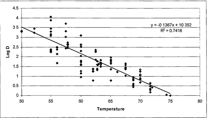
2.2.2 Thermal death kinetics of pathogenic microorganisms ... 48

2. 3 Exposure Assessment ... 48

2.3 .1 Cons'umption Patterns of Dairy Products in Australia ... .48

2.4 Risk Characterisation ... 49

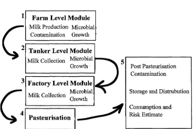
2.5 Model Development ... 49

Sources of Hazards at the Farm Level.. ... .49

Overview ... 50

2.5.1 Farm Level Module ... 52

2.5.2 Milk Collection and Transport Module ... 56

2.5.3 Factory Collection ... 59

2.5.4 Pasteurisation ... 61

~. RE~ULT~

...

()"°

3.1 Hazard Identification. ... 64

3.2 Hazard Characterisation ... 64

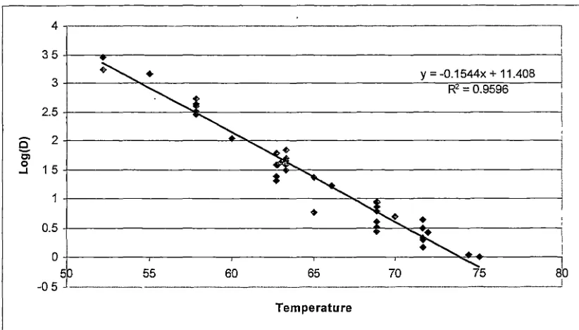
3.3 Thermal death kinetics of pathogenic microorganisms ... 64

3.4 Consumption patterns of daily products in Australia ... 70

3. 5 Model Inputs ... 77

3.6 Farm Level Module ... 79

3. 7 Milk Collection and Transport Module ... 81

3.8 Fact01y Level Module ... 83

3.9 Pasteurisation Module ... 84

~- DI~CU~~ION

...

~ti 4.1 Assumptions and Methods ... 86

4.2 Hazard identification ... 89

4.3 Thermal inactivation of bacterial pathogens ... 90

4. 4 Consumption patterns ... 91

4. 5 Model implementation and estimates ... 9 2 4. 6 Further Avenues for Research. ... 94

:5.

CONCLU~ION~

...

!>()

Notes on Modelling ... 96

Risk assessment -A modeller's view ... 97

<i.

REFERENCE~

...

~~

APPENDICES ... 108

Appendix A. NSW Dairy Industry Survey ... 109

Appendix B Profile of the Australian population's health ... 113

Appendix C Complete data set for bacterial thermal inactivation ... 121

Abstract

This thesis describes the development of a food safety risk assessment framework for the Australian dairy industry, through the collection of specific information regarding that industry and its collation and organisation into a structured and flexible spreadsheet model. The risk assessment model framework was developed for use as a tool for evaluating, identifying and prioritising research needs. Developed in Excel (Microsoft Corp.) with @Risk (Palisade Corp.) as an add-in, the model uses a stochastic approach to evaluate the likely concentration of hazards that may be present in liquid milk. Those hazards include: Escherichia coli, Listeria monocytogenes, Salmonella spp., Campylobacter spp., Staphylococcus aureus and Yersinia enterocolitica, Bacillus cereus, antibiotic and herbicide residues. The structure of the model allows for multiple hazards to be modelled in a single simulation. Flexibility of the spreadsheet model allows for manipulation of the input distribution 'parameters. This enables the evaluation

1. Literature Review

1.1 Introduction

The trend in the incidence of food borne illness (FBI) in developed countries is, at present, unclear. The US Centre for Disease Control (CDC) has recently reported a decrease in the proportion of FBI attributed to bacterial infection for the year 2001 (CDC, 2002). However, in general FBI has been increasing over the last 10-20 years (CDN, 2000). The increase in illness could be an artefact of better epidemiological data, better diagnostic techniques (including laboratory tests) or a true increase in the number of pathogenic organisms present in foods. Due to the increase in illness, various

governmental, international and industry organisations are targeting the cause of the increase.

FBI causes economic and social consequences, and with changes in social trends, e.g. increased reliance of consumers on other people to prepare food, attempts at curbing the increase in FBI have led to new areas of research, including processing and

production changes, the widespread implementation of hazard analysis and critical control point (HACCP) scheme on a larger scale and also the increasing emphasis on Risk Assessment, and in particular food safety risk assessments.

Risk assessment is a field of science that has grown in recognition and use over the last 30 years. It has application in many disciplines including: medicine, finance, cancer research, computing and microbiology (Haas et al, 1993; Soh et al, 1995; Brown et al, 1998; Cassin et al, 1998; Smith 1988)). Risk assessment is an applied science formed by the confluence of several disciplines. Risk assessment in microbial food safety therefore involves elements of microbiology, epidemiology, statistics, computing; pathobiology etc. In the management of food supply, risk assessment has been adopted

as a structured process for organising scientific knowledge about hazards, so that inferences can be made about the likelihood of a particular food safety event occurring because of ingestion of a hazard and the impact of this in terms of severity of illness or some social or economic measure of consequence. The assessment may be either qualitative, where data is lacking and value judgements are required, or quantitative when there is sufficient data to describe the process mathematically and the likelihood of events described in terms of numerical estimates of probability (Waltner-Toews and McEwen, 1994a). The estimate of the probability of those events should include the variability and uncertainty of those estimates based on the information available

- '

regarding the events (Nauta, 2000).

Institute (ILSI, 2000) and the Codex Alimentarius Commission (CAC, 1998) have

developed standardised frameworks for conducting microbial food safety risk

assessments. The US Environmental Protection Agency has developed a framework for

environmental risk assessments (EPA, 1998), and the Office International des Epizooties

(OIE, 1998) has developed a risk assessment framework for appraising the risk of

hazards to animal, plant and human health in imported foods and agricultural

commodities. These frameworks are not intended to be absolute rules; rather they are

aimed at being useful guidelines that cover the key aspects within the risk assessment

process.

The concurrent existence of several frameworks for performing risk assessments

creates potential for confusion. However the approach adopted by each framework is

fundamentally the same, there being minor differences in detail. To avoid confusion

arising from terminology this document adopts the framework and definition proffered

by the Codex Alimentarius Commission (CAC, 1998). These have been implemented

during international collaborations of scientists performing a range of risk assessments

of pathogens in foods (USDA/FSIS, 1998; WHO/FAO, 2001) and therefore have the

most credibility to adopt as a standard. The definitions are as follows:

Hazard Identification: The identification of chemical, microbiological or physical

agents that may cause adverse health affects in humans through the consumption of, or

exposure to, a particular food product or type.

Hazard Characterisation: A qualitative or quantitative description of the nature of

the adverse reaction associated with the chemical, microbiological and physical hazards

that may be present in the food.

Exposure Assessment: The qualitative or quantitative estimate of the likely intake

of chemical, microbiological or physical hazards through the consumption of food, or

other routes if applicable.

Risk Characterisation: The qualitative or quantitative evaluation of the probability,

including uncertainty, of the potential harm and the severity of that harm to the health of

the consuming population based on the above steps.

These four steps form the basis of risk assessments designed to comply with the

internationally accepted approach proffered by the World Health Organisation (WHO)

and the Food and Agriculture Organisation (FAO; CAC, 1998). Individual risk

assessments may differ in the detail of the approach taken, but in broad terms comply

with the above structure and process. To clarify the application of the above process

when dealing with a food borne hazard a more detailed explanation of each step in risk

1.2 Risk Communication

Risk communication is as vital to the success of a risk analysis as the four components of risk assessment. Regardless of how accurate and reliable the prediction that the risk assessment provides, if decision and policy makers do not understand what those predictions mean and what their limits are then problems may arise in the application of the assessment. Risk communication is an interactive exchange of ideas, information and opinions between the risk managers and the risk assessors and the stakeholders (i.e. those affected by the risk), which should occur throughout the assessment process. This is not a once off process. There should be continual

interaction and communication throughout the risk assessment process (Notermans et al,

1999).

1.3 Risk Management

With adequate communication of the findings of a risk assessment the final step in the process may occur; the management of those risks identified during the assessment, taking into account the current policy and regulations that exist (Notermans et al, 1999). This falls outside the hands of the scientific community and into the realm of the regulators and policy makers. There are three effects that may be brought about, although not exclusively: the managers decide to do nothing; action is taken to reduce the risks identified in the assessment, or initiation of further research. The first of these may be considered a frustrating outcome, however, having established the conditions that enable a particular risk from a hazard(s) to arise, any change in those conditions may be

monitored and at a later date some action may be made. The second, would generally arise if the risk was considered by the managers to be too great, hence the need to take action to reduce it. The third acknowledges that even the most carefully constructed risk assessment contains untested assumptions that may be erroneous or simply critical to the outcome, and usually will have identified data gaps in our knowledge of a process

that, if available, would enable a clearer picture to be obtained.

1.4 Uncertainty

With any attempt to determine the amount of hazard, especially microbiological, at the point of consumption one must consider the variability inherent in the process. Delignette-Muller and Rosso (2000) showed that both uncertainty and variability should be accounted for in any attempt to analyse the degree of exposure to Bacillus cereus in pasteurised milk at the point of consumption. Any ~odel that is used to describe the process of growth and, or inactivation should address both uncertainty and variability (Nauta, 2000; WHO/FAO, 2002).

Before a risk assessment on a particular pathogen can be produced, extensive knowledge of the organism is required including: growth rates, optimal conditions,

effects of bacteriostatic and bacteriocidal agents and ability to grow and or produce toxins in food. All these aspects produce a profile of the pathogen, and with this information a clearer picture can be gained as to the foods in which the bacterium is

likely to survive and/or grow.

A large part of producing a risk assessment is the ability to describe all the aspects of the risk in terms of mathematical functions, to give a numerical value to the risk. The form that this takes is a model that can be either deterministic or stochastic. A deterministic model uses point estimates rather than a range of possible values and their associated probabilities as are used in stochastic modelling. From this background it is possible to make decisions that can affect a wide range of areas, from the incidence of illness to the introduction of diseases to a "clean" area. The latter point is especially pertinent with the current efforts to open trade between all countries in the world and to have a global standard for food (ICMSF, 1998).

The biggest stumbling bock for the evaluation of potential sources of

contamination and the degree of that contamination is a lack of reliable and detailed data (Jaykus, 1996). However, as with other problems regarding a lack of data, a qualitative estimate may sometimes be used rather than a quantitative one.

1.5 Stochastic Modelling

(Buchanan et al, 2000). However, there is also an amount of information that is not known nor can ever be known. This is uncertainty. There are three types of models that may be used when attempting to model a system, primary, secondary and tertiary. Tertiary models are beyond the scope of this project. Primary models describe the effect of a single variable on the system, e.g. temperature on the rate of growth of microorganisms (van Gerwen and Zwietering, 1998). Secondary models attempt to include both variable and uncertain aspects of a process into the model, thus in this example giving a range of values for the growth rate at a specified temperature. A large part of stochastic modelling is to reduce the uncertainty, and more accurately describe variability (Cassin et al, 1998).

The range of possible values that any particular variable can take is described by a

distribution function in stochastic models. As with the type of model used, distribution functions can be either discrete, taking only a set of specific values, or continuous, having a range of real values (Vose, 1998). Determining the result of mathematical operations between distribution functions is not an easy task, requiring a deep

understanding of the mathematics behind the functions

01

ose, 2000). To overcome the problem of the difficulty in working with distribution functions, stochastic modelling uses sampling from within each distribution to obtain a final predicted value. A process automated by computer software. Hence the final output of a stochastic model is limited by the technique used to sample the range of distributions for each variable and the number of samples taken. The more samples used, the better the accuracy of the predicted values. Two commonly used sampling methods that can be used to produce a predicted value from a model are Monte-Carlo and Latin Hypercube (Vose, 1998; Cassin et al, 1998). The Monte-Carlo sampling technique takes random samples from the entire distribution of possible values, whereas Latin Hypercube sampling divides the distribution into equal parts and takes an equal number of samples from each part of the

distribution. In both cases the distribution function will be re-created with sufficient iterations, although the Latin Hypercube technique will take fewer iterations than the Monte-Carlo technique (Vose, 1996). An iteration in a stochastic model is selection of a single sample from each of the distributions in that model.

1.6 Hazard Identification

A hazard can be defined as an agent which is either infectious or otherwise that may cause an adverse health effect. In food safety, a hazard is a contaminant of or an element of the food itself. The hazard in food may cause an adverse health affects when ingested by a person. Hence, there is a very broad range of hazards that may possibly be present in a particular food. Comprehensive assessment of all the risks for a particular food product may thus be very time consuming and difficult and most risk assessments consider a subset of the possible classes of hazards.

There are three main groups of hazard that may be found in foods, these include microbiological, chemical, and physical. A fourth group, product tampering, may be included although this should be classed as a risk as the tampering will affect the level of

hazard in the product. This risk falls outside the scope of this risk assessment, however it should not be discounted entirely due to potentially disastrous effects. The reader should be aware that this is another source of contamination of the product.

Hazard identification is mainly a qualitative evaluation of the risk issues being estimated in the risk assessment. For microbial risk assessment hazard identification is

often a straightforward task as the agents responsible for causing adverse reaction are well described and their effects on consumers can be measured in terms of hours or days (Lammerding and Fazil, 2000). Hazard identification for microbial pathogens is more focussed on determining those organisms that are likely to be present in the product of concern, in this case dairy products, rather than determining if there is a possible health effect induced from the ingestion of the organism (Lammerding, 1997). Chemicals, however, represent a seemingly inexhaustible supply of hazards. Moreover the effects of these contaminants in foods on the exposed population is usually measured in terms of years or lifetimes, making the evaluation of the risk from these

hazards a difficult task. As a result there have been risk assessments performed for single chemical hazards to determine whether they have a heal~ effect (Waltner-Toews et al, 1994a; Welp and Brummer, 1997).

organisms. A description of each of these pathogens would be a lengthy process and for several of the organisms listed there is a paucity of information in the published literature regarding their characteristics and modes of transmission and virulence. It will be noted by the reader that in the Hazard characterisation section (1.3) there are not 70 organisms described, rather, several of the more significant organisms have been highlighted for discussion.

Hazards identified as being of concern in this study, as elicited from discussions with experts and stakeholders in the Australian dairy industry, are shown in decreasing

order of priority in Table 1.10. Included in the list are some hazards that have not been examined in this thesis, as there is insufficient information available to model the health risks arising from their occurrence in dairy products. The higher priority hazards are described briefly below.

1. 7 Pathogens of concern in the dairy industry

Listeria monocytogenes

monocytogenes is a pathogen of concern, as can be perceived by Australia's and

the FDA' s policy of "zero tolerance" for the organism in ready-to-eat (RTE) foods (Shank et al, 1996; Duffes et al, 1999). It is ubiquitous in the environment, and relatively harmless for the majority of people. It does, however, have one of the highest mortality rates for all pathogenic bacteria, up to 30% (Gray and Killinger, 1996; Doyle et al, 1997). Incidence estimates for listeriosis range from 7.1 per million population per year in the US (Gellin et al, 1991) to between 0.1 and 11.3 per million per year in Europe (Notermans et al, 1998). In Australia there were 60 cases of listeriosis in 2000, ,...,3 cases

per million population, with two outbreaks of food borne listeriosis with 13 cases in Australia between 1980 and 1995 (CDN, 2000). Table 1.1 outlines the main

characteristics of listeriosis. Several dose response relationships have been developed for this pathogen and are outlined in section 1.8, below.

Escherichia coli

Escherichia coli 0157:H7 was first recognised as a human pathogen in 1982

(Riley et al, 1983 ). Its importance as a human pathogen has grown over the last twenty years. There are many pathogenic strains of E. coli, each with different disease characteristics (Murray et al, 1998). Among the enterohaembrrhagic strains, the so-called verotoxigenic E. coli (VTEC) or shiga-toxin producing E. coli (STEC) group, E.

coli 0157:H7 is found predominantly overseas, whereas 0111 is the most common

enterohaemorrhagic E. coli infections. Dose response relationships have primarily focused on E.coli 0157:H7 and there is a lack of information available regarding other

E. coli strains to produce suitable dose response models.

Table 1.1 Characteristics of Listeriosis (CDC, 200la)

Clinical Features Manifestations are host dependent. In elderly and

immunocompromised persons, sepsis and meningitis are the main !Presentations. Pregnant women experience a mild, flu-like illness often !followed by foetal loss or bacteraemia and meningitis in their

111ewboms. Immunocompetent persons may experience acute febrile gastroenteritis.

Etiologic Agent !Listeria monocytogenes

Incidence !Approximately 3 cases per million population annually in Australia. Transmission Contaminated food. Rare cases of nosocomial transmission have been

Ire ported.

Risk Groups For invasive disease, immunocompromised individuals, pregnant iwomen and their foetuses and neonates, and the elderly.

Table 1.2 Characteristics of verotoxigenic, or ST E. coli

infections (CDC, 2001 b)

Clinical IAcute bloody diarrhoea and abdominal cramps with little ~r no fever; Features usually lasts 1 week.

Etiologic Agent Several, most recognised is Escherichia coli serotype 0157:H7. Gram-negative rod-shaped bacterium producing Shiga toxin(s). Sequelae Haemolytic uremic syndrome (HUS): People with this illness develop

kidney failure and often require dialysis and transfusions. Some develop chronic kidney failure or neurological impairment (e.g., seizures or blindness). Some require surgery to remove part of the bowel. Death (estimated 61 fatal cases annually; 3-5% with HUS die). Costs Estimated 20 cases annually in the Australia. The illness is often

misdiagnosed; therefore, expensive and invasive diagnostic procedures may be performed. Patients who develop HUS often require

prolonged hospitalisation, dialysis, and long-term follow-up.

Transmission Major source is ground beef; other sources include consumption of un-pasteurised milk and juice, sprouts, lettuce, and salami, and contact with cattle. Waterbome transmission occurs through swimming in contaminated lakes, pools, or drinking inadequately chlorinated water. Organism is easily transmitted from person to person and has been difficult to control in child day-care centres.

Salmonella

The genus Salmonellae is now considered to contain a single species, Sabnonella

enterica, with seven distinct subgroups. This species contains over 2000 serovars all of

which are capable of causing infection and disease in humans (Murray et al, 1998; Fazil et al, 2000). In Australia there were around 5700 reported cases of Salmonellosis in total in 2000 (CDN, 2000). Foodbome salmonellosis in Australia, between 1980 and 1995, caused 27 outbreaks with 1323 cases and one death (CDN, 2000). Table 1.3 outlines the main characteristics of salmonellosis. This highlights the importance of this organism in the food industry, as it covers many food types, countries and situations.

Teunis et al (1999) reported that one of the biggest complications with modelling the dose response relationship for Salmonellae is the difference in strain virulence within the species. This strain difference makes it difficult to describe a dose response for

Salmonellae, because it should be known for which strain the dose response has been

derived. Consequently several dose response relationships have been developed for this pathogen; see section 1.8.

Table 1.3 Characteristics of Salmonella spp infections (CDC, 200lc)

Clinical

!Fever, abdominal cramps, and diarrhoea (sometimes bloody). Features Occasionally progresses to sepsis.

Etiologic Agent _{Enterobacteriaceae of the genus Salmonella. Approximately 2000} serotypes cause human disease.

Transmission _{Contaminated food, water, or contact with infected animals.}

Risk Groups Affects all age groups. Groups at greatest risk for severe or complicated disease include infants, the elderly, and persons with compromised immune systems.

Campylobacter jejuni

Campylobacteriosis is one of the most common causes of intestinal disease (Medema et al, 1996) with estimates of incidence ranging between 1-2% in the Netherlands (Medema et al, 1996), "'1 % in the US (Tauxe, 1992), and 1.1 % in the UK (Kendall and Tanner, 1982). In Australia there were "'12000 notified cases of campylobacteriosis in the year 2000. Between 1980 and 1995 there were 5 outbreaks involving 109 cases of foodborne campylobacteriosis (CDN, 2000). The majority of cases of campylobacteriosis are sporadic. Table 1.4 outlines the main characteristics of

Campylobacter jejuni infections. Several dose response models have been published,

[image:16.569.61.502.99.463.2]

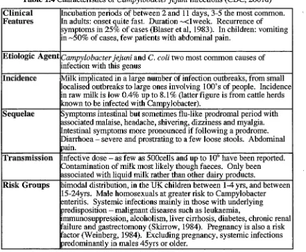
Table 1.4 Characteristics of Campylobacter jejuni infections (CDC, 2001d)

Clinical Incubation periods of between 2 and 11 days, 3-5 the most common. Features In adults: onset quite fast. Duration "-"<1 week. Recurrence of

symptoms in 25% of cases (Blaser et al, 1983). In children: vomiting in ,_,50% of cases, few patients with abdominal pain.

Etiologic Agent _{Campylobacter jejuni and} C. coli two most common causes of

infection with this genus

Incidence Milk implicated in a large number of infection outbreaks, from small localised outbreaks to large ones involving lOO's of people. Incidence in raw milk is low 0.4% up to 8.1 % (latter figure is from cattle herds known to be infected with Campylobacter).

Sequelae Symptoms intestinal but sometimes flu-like prodromal period with associated malaise, headache, shivering, dizziness and myalgia.

ntestinal symptoms more pronounced if following a prodrome. Diarrhoea - severe and prostrating to a few loose stools. Abdominal pain.

Transmission nfective dose-as few as 500cells and up to 106

have been reported. Contamination of milk most likely though faeces. Only been

associated with liquid milk rather than other dairy products.

Risk Groups bimodal distribution, in the UK children between 1-4 yrs, and between 15-24yrs. Male homosexuals at greater risk to Campylobacter

enteritis. Systemic infections mainly in those with underlying predisposition - malignant diseases such as leukaemia,

immunosuppression, alcoholism, liver cirrhosis, diabetes, chronic renal failure and gastrectomony (Skirrow, 1984). Pregnancy is also a risk

actor (Weinberg, 1984). Excluding pregnancy, systemic infections predominantly in males 45yrs or older.

Bacillus cereus

Bacillus cereus is a Gram-positive, spore-forming bacterium, found in most

environments, from soil to the raw ingredients in foods. It is recognised as a food borne pathogen and is a significant causative agent in food born illness, due to either of two toxins produced by the organism (Dufrenne et al, 1995; Murray et al, 1998). In Australia between 1980 and 1995 there were 5 outbreaks of food borne B. cereus

infections, involving 27 cases (CDN, 2000). More recently the organism has been implicated in an outbreak in Victoria (Vic. DHS, 2002). The two toxins produced by B.

cereus cause differing illness. A heat stable toxin is associated with the emetic form of

illness, and a heat labile toxin is associated with the diarrhoeal form (Murray et al, 1998). Table 1.5 outlines the characteristics of B. cereus intoxications.

Notermans et al (1997) describe the risk assessment process for B. cereus in pasteurised milk. From various sources, they state, that the likely level of the organism required to induce symptomatic illness is >105• This is a similar figure to that presented

by Doyle et al (1997), who indicate that an infectious dose of this organism is between 105

-107 and 105 -108

food, respectively. Those authors did not derive a dose response relationship for the organism. A lack of information regarding this organism's ability to induce illness, indications that not all strains of B. cereus are toxin producers, and differences between

[image:17.570.64.489.218.516.2]

the level of organism required to cause either emetic and diarrhoeic illness are highlighted as difficulties in developing a suitable dose response relationship for this organism.

Table 1.5 Characteristics of Bacillus cereus infections (adapted from Murray et

al, 1998).

Clinical Diarrhoeal and emetic food poisoning a result of two different toxins Features

Etiologic Agent Bacillus cereus - toxin production. ·

Incidence No cases of B. cereus poisoning have been reported for UHT milk,

but is a common contaminant of dried milk, although the importance of this is under debate.

Sequelae Diarrhoeal - incubation period of 8-16 hours, followed by abdominal cramps, and profuse diarrhoea. Vomiting and fever are occasional symptoms, recovery usually within 24 hrs. Emetic poisoning short incubation of 1-6 hours. Nausea followed by vomiting and malaise, recovery generally within 24 hours.

Transmission Associated with the spoilage of fresh milk, this has changed recently !due to the introduction of refrigeration for pasteurised products, and !Partly from reduced incidence of contamination of raw materials. Can

still be readily isolated from pasteurised milk (Christiansson, 1989) and cream. Can also be isolated from UHT milk (Mostert et al, 1979;

MT

esthoff and Dougherty, 1981)

Risk Groups No particular groups are at risk, although the extremes of age and immunocompromised would have a relatively higher risk of infection. Most commonly associated with large-scale food preparation.

More complete lists of potential pathogens in dairy products are presented in Boor

[image:18.570.55.504.86.450.2]

Table 1.6 Staphylococcus aureus: characteristics of disease

Clinical Features Symptoms usually appear within 2-4 hours (Bergdoll, 1979). Symptoms generally persist for less than 24 hours

Etiologic Agent Staphylococcus aureus

Incidence USA of 131 outbreak and over 7000 cases (Holmberg and Blake, 1984). Reported cases of staphylococcal food poisoning from cheese limited to cheddar and similar varieties (ICMSF, 1980, 1986) and Swiss type cheese (Todd et al, 1981).

Sequelae Nausea, retching, vomiting and less frequently diarrhoea. Fever has been found in ,..,16% of cases (Holmberg and Blake, 1984). With severe cases - dehydration, shock and collapse, accompanied by shallow breathing and weak pulse. Up to 10% of sufferers seek medial attention. Death rare. Symptoms may be confused with B.

cereus emetic infection (Newsome, 1988)

Transmission Milk from most species including cattle (Harvey and Gilmour, 1985), goats and sheep contain S. aureus. Greater numbers in mastitic milk,

although less marked with this organism than other mastitis causing bacteria, S. uberis (Bramley et al, 1984). Presence in raw milk is

generally not a problem, though from mastitic milk higher numbers of enterotoxigenic organisms may be present (Lombai et al, 1980). There have been examples of toxin production in milk prior to pasteurisation (Holmberg and Blake, 1984). Staphylococcus aureus can be isolated from a wide range of fermented milk products, usually in low

numbers. The greatest numbers is generally in hard cheeses (cheddar etc) due predominantly to a poor starter culture.

Risk Groups Wide variation among normal adults, but greatest susceptibility in the young and old. Unhealthy people are at greater risk, but no particular predisposing condition for staphyl_ococcal infection.

Table 1.7 Characteristics of Group A Streptococcal infections (CDC, 2001f)

Clinical Features Non-invasive disease (strep throat, cellulitis); invasive disease (necrotizing fasciitis (NF), streptococcal toxic shock syndrome

(STSS), bacteraemia, pneumonia); nonsuppurative sequelae (rheumatic fever, post-streptococcal glomerulonephritis). STSS is a severe illness characterized by shock, multiple organ failure. NF presents with severe local pain, destruction of tissue. Rheumatic fever is a leading cause of acquired heart disease in young people worldwide.

Etiologic Agent Group A Streptococcus; STSS and NF occur more often among

persons infected with group A Streptococcus spp serotypes M-1 and

M-3 or toxin- producing strains.

Incidence Approximately 10,000 annual cases of invasive disease (3.7/100,000 population) occurred in 1998; approximately 5% are STSS and 5%-8% are NF. Over 10 million noninvasive GAS infections (primarily throat and skin infections) occur annually.

Sequelae Death in 10%-13% of all invasive cases, 45% of STSS, 25% of NF cases. Organ system failure (STSS) and amputation (NF) also may result.

Transmission Person to person by contact with infectious secretions.

Risk Groups Invasive disease: elderly, immunosuppressed, persons with chronic cardiac or respiratory disease, diabetes, skin lesions (i.e. children with varicella [chicken pox], intravenous drug users) African-Americans, American Indians. Noninvasive disease: children (especially

[image:19.568.64.490.99.504.2]

Table 1.8 Characteristics of Group B Streptococcal infections (CDC, 2001g)

Clinical Features OCn neonates: sepsis, pneumonia and meningitis. In adults: sepsis and soft

~issue infections. Pregnancy-related infections: sepsis, amnionitis, !Urinary tract infection, and stillbirth.

Etiologic Agent

Streptococcus agalactiae or group B streptococcus (GBS).

Incidence !Approximately 18,000 cases occur annually in the United States;

approximately 7,500 occurred in newborns before recent prevention. [he rate of neonatal infection has decreased from 1.7 cases per 1,000 Hve births (1993) to 0.6 cases per 1,000 live births (1998).

Sequelae Neurological sequelae include sight or hearing loss and mental

retardation. Death occurs in 6% of infants and 16% of adults.

Transmission !Asymptomatic carriage in gastrointestinal and genital tracts is common.

fotrapartum transmission via ascending spread from vaginal and/or gastrointestinal GBS colonization occurs. Mode of transmission of disease in non-pregnant adults is unknown.

Risk Groups Risk Groups Adults with chronic illnesses (e.g., diabetes mellitus and

liver failure), pregnant women, the foetus, and the newborn are at risk. For neonatal disease, risk is higher among infants born to women with OBS colonization, prolonged rupture of membranes or pre-term delivery.

Table 1.9 Characteristics of Yersinia enterocolitica infections (CDC, 2001e)

Clinical Features Children - fever, abdominal pain, and diarrhoea, which is often bloody. !Adults - right-sided abdominal pain and fever. Symptoms develop within 4-7 days. Duration of illness 1-3 weeks, maybe longer

Etiologic Agent Most illness caused by Y. enterocolitica. Y pseudotuberculosis causes similar illness though not as common.

Incidence 1 per 100000 people, more common in children and during winter

Transmission Animal reservoir primarily pigs, also rodents, rabbits, sheep, cattle,

horses, dogs, and cats. Contaminated milk or untreated water, contact

Table 1.10 - Ranking of Hazards Associated with Dairy Products Hazard Ranking Hazard

High Enterococci; EHEC/VTEC; Salmonella spp.; Listeria monocytogenes; herbicides; aflatoxins .

Medium Yersinia spp.; Campylobacter spp.; Bacillus cereus;

Staphylococcus aureus; Cryptosporidium spp; antimicrobials;

antiparasitics - flukicides and anthelminthics ; mycotoxins Pesticides - Organochlorines, Organophosphates and pyrethroids

Low Q Fever; Toxoplasmosis; Brucella abortis; Pseudomonas pseudomallei; Clostridium botulinum; Clostridium perfringens;

BST and other hormones; Blue-green algae; Heavy metals and Iodine

For consideration if Mycobacterium paratuberculosis; Bacillus anthracis; Viruses; time is available agent causing bovine spongiform encephalopathy (BSE);

enzootic bovine leucosis (EBL)

Of these hazards it was resolved (see section 2.1) that those to be included in the

risk assessment model be: Escherichia coli, Salmonella spp, Listeria monocytogenes,

Bacillus cereus, Campylobacter jejuni, Yersinia enterocolitica, antibiotics and herbicides

in general (there was insufficient information to focus on a particular one).

1.8 Hazard Characterisation - Dose Response Assessment

Hazard characterisation, as mentioned previously, is the qualitative or quantitative description of the adverse health effects resulting from contact with those hazards identified in the hazard identification (Farber et al, 1996; Buchanan et al, 2000). Buchanan et al (2000) mentions the infectious disease triangle, stating the importance of three aspects of the likelihood of developing illness from a foodbome pathogen. These

three aspects include the interaction between the host, the pathogen and the food matrix, which together determine if illness is manifested in the host. The three points in the disease triangle are:

•

The disease causing characteristics of microorganisms; infections, toxico-infectious or toxigenic.

• The characteristics of the host; the very young, the old, immunocompromised, immune or naive.

• The food matrix: the food may ·confer some resistance from the host's non-specific and immune system defences to the pathogen, it .may either hamper or enhance the pathogenicity of the organism.

It is not necessary here to describe the wide and varied forms of pathogenicity of microbiological hazards or to give a detailed examination of the chemical hazards (This alone could constitute a third of this thesis). For clarity, however, a brief discussion of the various forms of dose response models that have been developed for both microbiological and chemical hazards shall be given, and then an examination of each prioritised hazard together with their dose response relationship, if that exists.

1.8.1 Dose Response Assessment

Dose response modelling is not a new concept. One journal article, describing

mathematically the infectivity of the tobacco mosaic virus (Furomoto and Mickey, 1967), is more than 30 years old and forms the theoretical basis of many of the models used currently. The basis of dose response modelling for food safety risk assessments, th~t is determining/predicting human health effects to known levels of hazards in a

mathematical form, has not changed. There have been a large variety of dose response papers published. These consider topics including: cancer research (Edler and Kopp-Schneider, 1998), chemical safety (Krewski and van Ryzin, 1981; Welp and Brummer, 1997), microbiology (Buchanan et al, 2000; Haas et al, 2000; Havelaar et al, 2000), water safety research (Regli et al, 1991; Haas et al, 1993), discussions on dose response modelling (Coleman and Marks, 1998; Buchanan et al, 2000), and papers discussing the advantages and disadvantages of different dose response models (Holcomb et al, 1999; Teunis and Havelaar, 2000; WHO/FAO, 2002).

There are many different ways to model the health reaction to the ingestion of known hazards. For microbial dose response models there are predominantly two end points that are modelled: the probability of infection and the probability of illness. A third endpoint that may be mentioned, though rarely modelled, is the probability of

mortality at a given dose, or it may be presented as severity with mortality included. Most studies only examine one of the end points, whereas a few try to make some connection between infection and the probability of developing illness from that

Dose Response Modelling Theory

The aim of dose response modelling is to determine the probability of a defined adverse health reaction from the ingestion of a particular hazard. Of the dose response models that have been developed, there are two broad categories: those models that assume a threshold, below which no infection occurs, and hit-theory models, which assume that every individual cell or toxic particle is capable of causing infection in the host (Furomoto and Mickey, 1967; Turner, 1975; Coleman and Marks, 1998). Much debate over which type of model is the most suitable has occurred. The majority of models used are hit-theory models, which are in a class of a larger group of mechanistic models. A single hit model assumes that a single particle is capable of causing an

adverse health reaction. The log-logistic, log-probit and Weibull (-Gamma) models are among the hit theory models used (WHO/FAQ, 2002). There has been confusion about which models are and are not hit theory models. For example the exponential model 'has

often been considered a threshold model due to the sigmoidal shape of the response curve, which suggests that below some level there is no response, however, Buchanan et al (1997) show that when the log is taken of the probability of response, there is a linear relationship between the log dose and the log probability. This precludes the possibility of a threshold existing for this model. Moreover, for another widely used model, the Beta-Poisson model, it has been demonstrated (Teunis and Havelaar, 2000) that although it is assumed to be a single hit model, it is not.

What follows is a brief discussion on the various forms of dose response models that exist in the published literature, the relationship between different models, and problems associated with each.

The underlying theme of hit-theory models assumes that each ingested pathogen

or unit of hazard is capable of causing disease, with some probability (Vose, 1998). This is a Binomial process; hence the probability of infection is given by:

(1)

Where Pin/ is the probability of infection, n is the amount of hazard ingested (trials), and p is the probability that each organism ingested will survive to cause infection.

The simplest of the dose response models that are used in the literature is the exponential model. The exponential model assumes that each organism entering the host is capable of causing infection, i.e. a single hit is required to cause infection, that each ingested cell acts independently of others, and that the organisms are distributed randomly throughout the contaminated food. The model is expressed in the form:

Where r is probability of an individual cell causing infection and d is the dose (number of organisms ingested).

The cells ingested in each dose are assumed to follow a Poisson distribution, randomly distributed, and the dose is the mean of the sample taken from that distribution (Powell et al, 2000). A further assumption in the exponential model is that r is a constant. This represents the host-microbe interaction, or the proportion of organisms surviving the host's defences to cause infection (Regli et al, 1991; Powell et al, 2000).

If r is not a constant, by taking a general case it's value can be approximated

(Vose, 1998). The Beta-Poisson model does this where it is assumed that r follows a Beta distribution (r

=

Beta(a, b)). This may be explained in terms of the ingested cells and the host's immune response. For each individual cell in the dose, each may be

considered independent, that is they all have equal probability of surviving to cause infection once inside the host. However, the number of cells in the dose that survive and are able to initiate infection can be described by a Beta distribution (Holcomb et al, 1999; Powell et al, 2000). The general form of the Beta-Poisson model is expressed as:

p = 1- (1 + d/bya (3)

This only holds for when b is much larger than a, and hence the probability of an

individual cell causing infection is low (Vose, 1998). The more common form of this is to express b in terms of the median effective dose (ED₅₀) or median Infective dose

(ID50), that is, the number of ingested organisms required to cause infection in half of the exposed population, where:

b = ED₅₀/(211

a - 1) (4)

Hence the Beta-Poisson model (3) can be expressed as:

P = 1 - (1 + (d/ED₅₀)* (211

a - l)ya (5)

Another approximation of the Beta-Poisson model may be made. Where b

approaches 0, the model (3) reduces to its Poisson form:

(6)

(7)

Where a, b and x are parameters affecting the shape of the curve.

This reduces to the Beta-Poisson model when x

=

1. Moreover, the

Weibull-Gamma reduces to the Log-Logistic when a= 1.

Other models have been used to describe the dose response relationship for

microbial pathogens. The ge~eral forms for these models are listed in Table 1.11.

Table 1.11 Dose response models used for microbial pathogens, general form

Model Parameters Equation

Logistic alpha, beta eaipna + oeca•m\OOSeJ I 1 + e acpna + oera-m\OOSeJ

Gompertz - log alpha, beta 1 _ e-eA(alpha + (beta*ln(dose)))

Gompertz - Power alpha, beta, power 1 _ e-e"(aJpha + (betaApower))

Log-Normal (Probit) alpha, beta Normal_cdf(alpha +beta* log₁₀(dose)

Multihit gamma,k Gamma_cdf(gamma *dose, k)

cdf = cumulative d1stnbut1on function

There are several considerations before a dose response model is used to predict

the probability of a health outcome. Firstly, the model should fit the observed data

adequately, and it should be as simple as possible (a more parsimonious model is one

that has fewer fit parameters than another which fits the data equally). The model

chosen should also be applicable over the range of conditions for the data to which it is

being applied (Holcomb et al, 1999). In the event that there is no suitable dose response

model available, with the exception of developing a new one, it has been proposed that

linear risk extrapolation can often be accepted as the default for dose-response curves

(Waltner-Toews and McEwen, 1994a).

Due to the broad range of models and hazards that have had a dose response

relationship described, the succeeding section details some models that have been

developed for microbial pathogens and presents a short treatise on the concept of

chemical dose response assessment.

I

1.8.2 Microbial Dose Response Assessment

There are several pathogens on which a greater amount of risk assessment

research has been focussed, namely E.coli 0157, Salmonella, Listeria monocytogenes

and to a lesser extent Campylobacter jejuni. Consequently for these pathogens there are

several papers that describe dose response models that have been developed. One of the

basic premises of these models is that at an increasing dose the chance ~f becoming ill

For each of the identified microbiological hazards a discussion on the various dose response models proposed to describe infectivity curves is presented. There are some microbial pathogens that have not had a dose-response curve defined. This is mainly due to a lack of data to describe the curve with any degree of certainty.

Listeria monocytogenes

Haas et al (1999) developed and validated a dose response relationship for infection for Listeria monocytogenes. Data used were based on animal feeding studies

conducted by Audurier et al (1980) and Golnazarian et al (1989). Haas et al (1999) used three different sets of data when fitting the parameters for the dose response

models. Hass et al (1999) compares the use of the exponential and the Beta-Poisson dose response models to fit the data used. Those authors found that the Beta-Poisson

model had the best fit to all sets of data, including the pooled dataset. A summary of the fit parameters is shown for the pooled dose response data (Table 1.12).

Buchanan et al (1997) developed a risk assessment model for listeriosis using German smoked fish data, as an example of the development of purposefully conservative risk assessment models based on annual disease statistics and food survey data. The dose response model used in that assessment was an exponential dose response model with parameter R being as conservative as the data would allow. The R-value estimated in the paper is defined as the probability that the ingestion of a single cell

of L. monocytogenes would produce an active case of listeriosis. This approach

estimates a "worst case", thus allowing the current tolerance to this organism's presence in foods to be evaluated. The dose response model was used to estimate an

adverse health effect, that is morbidity.

Lindqvist and WestOo (2000) used a similar approach as Buchanan et al (1997) to develop a conservative dose response relationship for Listeria monocytogenes based on

annual disease statistics and food survey data in Sweden. They selected two models: the exponential and the Weibull-gamma. The fitted parameters for the exponential model are shown in Table 1.8.2.1. The parameter values used in the Weibull-gamma model

were those estimated by Farber et al (1996).

Farber et al (1996) developed a dose response model for Listeria monotytogenes

based on the Weibull Gamma model. The parameter values fitted to the model are not presented, however, those authors attempted to distinguish between high and low risk populations, through the use of the infectious dose (ID) at two levels, ID10 and ID90• The IDn is that dose causing illness in the stated (n) percentage of the population, i.e. in the above case, 10% and 90% of the population respectively.

monocytogenes in ready to eat foods (WHO/FAO, 2001). An exponential model was

[image:26.570.110.468.439.653.2]

used for the dose response relationship, with different parameter values for susceptible and less susceptible exposed populations.

Table 1.8.2.1 Dose response model parameters for Listeria monocytogenes

Author Model Parameter Value

Haas et al (1999) Exponential k 1.77 x 104

Beta-Poisson _- 0.25

Nso 2.76x102 Buchanan et al Exponential R 1.179 x io-10 (1997)

Lindqvist ad Exponential R 5.6 x 10-10

Westoo (2000)

Farber (1996) Weibull-gamma b 1010·98 (high risk) 1010·26 (low risk)

WHO/FAO (2001) Exponential R 1.06 x 10-12 (susceptible) 2.37 x 10-14 (normal) N50 s1gmfies the dose at which half the exposed population will become mfected

R is the probability that the ingestion of a single cell causes the adverse health reaction

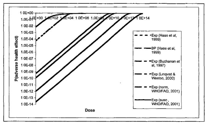
A comparison of the different dose response relationships that have been derived

for Listeria monocytogenes is shown (Fig 1.1). The curves presented are those that

could be regenerated from the information presented in the papers listed above.

1 OE-02

1 OE-03

~ 1.0E-04

"'

ii; 1.0E-05

E

..

1.0E-06

~ 1 OE-07

~ 1 OE-08

~ 1 OE-09

'O

~ 1 OE-10 1 OE-11

1.0E-12

1 OE-13

1 OE-14

Dose

- - - •Exp (Haas et al, 1999)

- - B P (Haas et al, 1999)

- - •Exp (Buchanan et al, 1997)

- - •Exp (Lmqv1st & Westoo, 2000)

- - •Exp (norm, WHO/FAQ, 2001)

- E x p ( s u s c , WHO/FAQ, 2001)

Fig 1.1 Comparison of different dose response models for Listeria monocytogenes.

Exp: exponential dose response model, BP: Beta-Poisson dose response model. Norm and Susc refer to the exposed population being either normal or susceptible to irlfections with this organism

Haas et al (2000) developed a dose response relationship for E. coli 0157:H7 based on an animal model for this organism from data produced by Pai et al (1986). This data was fitted to the beta-poisson dose response relationship, with validation based on outbreak data from the US. In this study the beta-poisson model goodness of fit (GOF) was compared with that of the exponential model. Haas et al (2000) state that although Shigella can be used in surrogate dose response modelling for E. coli 0157, the dose response relationship they present does not support the use of surrogacy between the two organisms. Intra-specific variability is inherent in all organisms, inter-specific variability, however, is greater. Regardless, there have been attempts to model

the dose response relationship for pathogenic E.coli with surrogate microorganisms, for example Shigella spp (Cassin et al, 1998). The dose response curves are reproduced in

Fig 1.2.

1.00E+OO

1.00E-M1 1.0E+12 1.0E+14·

1.00E-02

,

••

1.00E-03

,

..

'iii" 1.00E-04

,.

!/)

,

Cl>

1.00E-05

,.

:§

:::.

1.00E-06

_,

c..

,

---Exponential

1.00E-07

_,

•

_,

- - - ·Beta Poisson

1.00E-08

,

1.00E-09

1.00E-10

Dose

Figure 1.2 Comparison of the Exponential and the Beta-Poisson dose response curve for E. coli 0157:H7. Redrawn from equations presented by Haas et al (2000).

Cassin et al (1998) describe another dose response relationship for E. coli 0157:H7. This model is based on human feeding trials for Shigella dysenteriae and

Shigella flexneri. It assumes that the pathogenicity of shiga-toxin producing E. coli is

similar to that of the Shigella species. The difference between their dose response

An animal model was used to study the infectivity of E. coli 0157 in rats (Havelaar et al, 2000). The experimental design did not provide sufficient data to allow the development of a dose response relationship. Furthermore Havelaar et al (2000) did not highlight the problems associated with extrapolating an animal model-based dose response relationship to humans. Because of a lack of data in the published literature based on animal models for E.coli 0157 infection a description of the dose response relationship has not been included in this thesis.

Powell et al (2000) described the development of two different sets of dose response models for E. coli. The first used Shigella dysenteriae as a surrogate for

Shiga-toxin producing E. coli strains, the second used data from enteropathogenic E. coli (EPEC) strains. The data were derived from human feeding trials with

enteropathogenic E. coli (EPEC) and S. dysenteriae Type 1 (Levine et al, 1973; Levine et al, 1978; Bieber et al, 1998). Three models for each data set were fitted: the exponential,

the Beta-Poisson, and the Weibull-Gamma models. The fit parameters for those models are given in Table 1.13. Moreover, the aim of that paper was to describe an "envelope" dose response model for E.coli 0157:H7. An envelope model describes the highest and lowest dose response limits for infectious strains of E. coli, and then a mean dose

response curve is fitted. The model chosen for the envelope was the beta-Poisson, with the upper and lower bounds defined by the surrogate pathogen (upper) and EPEC (lower) model. The median value for the envelope was again a beta-Poisson DR model, with epidemiological data from various sources, primarily concerned with ground beef in

the USA. That model was the most complete, in terms of explanation of the process involved in generating the dose response curve, and provided a means of determining the variability in probability of infection between strains of E. coli. The dose response curves generated from the equations presented by Powell et al (2000) are presented (Fig 1.3. overleaf).

1 E-02

1 E-03

:J: 1 E-04

c:

8_ 1.E-05

~ 1 E-06 1 E-07

1 E-08

Dose

---Exp(a)

- ...,,BP(a)

WG (a)

~~''"' ~· "Exp (b) - - •BP(b)

- - - WG (b)

Figure 1.3 Comparison of the dose response curves for E. coli 0157:.H7

presented by Powell et al (2000). a, band c refer to datasets used to derive the dose

response curve (see table 1.13). Exp= exponential, BP= beta-Poisson, WG

=Weibull-Gamma

Haas et al (2000) show a greater degree of uncertainty in the low and high dose regions

of the curve with the beta-Poisson model than does the beta-binomial mode used by

Cassin et al (1998). The beta-binomial model used by Cassin et al (1998) gives a N₅₀ of

""3.2 x la3, whereas Haas et al's (2000) model gives the N₅₀ at "'6.3 x 105• The reasons

for this difference may arise from several sources; the data used, the method of

parameter fitting for determining the relationship; the strain of the bacterium used, or the

differences between the general form of the dose response curve described by the

beta-Poisson and beta-binomial models.

Salmonella

Teunis et al (1999) used the data collected from human feeding studies for

Salmonella enterica serovar Meleagridis to develop a dose response relationship for this

pathogen. The authors attempted to model both the dose response for infection and the

dose response for illness resulting from infection. Teunis et al (1999) used the

beta-Poisson dose response relationship to model the probability of infection. Fitting of the

dose response data resulted in the Beta-Poisson dose response model reducing to a

simple exponential model. Summarised in Table 1.14 are the parameter values fitted to

the dose response models.

Whiting and Buchanan (1997), using an exponential dose response relationship,

predicted that with an increase in prevalence of Salmonella Enteritidis in flocks of

chickens the probability of illness increases. They used parameter values derived by

Table 1.13 Summary of models for dose response relationship for

E. coli 0157:H7

Author Model Parameter Value

Haas et al (2000) Exponential P₁(D) 1- exp ~-D/k)

K 1.6 x 10

Beta-Poisson P₁(D) 1 - [(l

+

D/N₅₀(21

'- - 1))"(-a)]

a 0.49

ED so 5.96 x 105 Cassin et al (1998) Beta-binomial P₁(D) 1 - (1 - P1(l))D

Pi(l) Beta (a, j3)

a _0.267

j3 In j3 ,.., Normal (5.435, 2.47) Powell et al (2000) (a)

Exponential r 2.052 x 10-4

Beta-Poisson a 0.157

j3 9.169

ED so 742

Weibull a _0.040

gamma

j3 239.327

x 3.514

(b)

Exponential r 4.070 x 10-10

Beta-Poisson a _0.221

j3 3112348.268

ED so 68494661

Weibull a _1.944

gamma

j3 7409.340

x 0.418

(c)

Beta-Poisson a 0.221

j3 8722.480

EDSO 16643

..

P1(D) is the probability of Illness given a dose of D orgamsms Pi(I) is the probability of illness given a dose of I organism (a) denotes the model fit parameters for S. dysenteriae

(b) denotes the fit parameters for EPEC

(c) The median value for the envelope dose response model

ED50 is the dose required to cause symptomatic illness in half the exposed

population

model is not purely to demonstrate the goodness of fit of the model but as part of a demonstration of the risk assessment process, and its ability to quantitatively describe the production of eggs and the associated contamination with Salmonella Enteritidis.

1.0

0.8

-

c 0 0.6

;:; (,)

.e

g

0.4

a..

0.2

0.0 _b'!""""'!"'~~~----~---~----~

1.0E+OO 1.0E+01 1.0E+02

Dose

[image:31.569.77.488.77.336.2]

1.0E+03 1.0E+04

Figure 1.4 Dose response curve for Salmonella Enteritidis in liquid eggs.

(Reproduced from Whiting and Buchanan, 1997)

Brown et al (1998) also produced a risk assessment for Salmonella in chickens.

Those authors do not identify which serotype of Salmonella they chose for developing

the risk assessment; neither do they give adequate explanation of the model.

An animal model was used to study the infectivity of Salmonella Enteritidis in rats

(Havelaar et al, 2000). The data presented in that paper indicate a high infectivity of the rats by Salmonella Enteritidis, however the authors did not describe a mathematical dose

response relationship for this bacterium in rats. Lack of data precludes a description of

the dose response relationship.

Fazil et al (2000) compare three different dose response models, in a report for the PAO/WHO on the hazard characterisation, for Salmonella. The first details Fazil's

(1996) beta-Poisson dose response model for infection for non-typhoid Salmonella on both nai"ve and exposed people, based on feeding study data. The second outlines the dose response model developed in the USDA/FDA (1998) Salmonella Enteritidis risk

Table 1.14. Parameter values for dose response models for Salmonella

Author Model Parameter Value

Whiting and Exponential r 0.00752

Buchanan (1997)

Teunis et al (1999) Beta-Poisson _- 0.89

4.4 x 105

-Illness model P(illjinf) 1-(1 + _)-r 1

-D

-1.0 x 10-16

-r 3.4 x 108

Fazil et al (2000) Beta-Poisson _- 0.3136

3008

-Beta-Poisson _- 0.4059

(naYve)

5308

-USDA-FSIS Beta-Poisson _- 0.2767

(1998) (normal)

- Normal(21.159, 20) min: 0,

max: 60

Beta-Poisson _- 0.2767

(susceptible)

- - Normal (2.116, 2) min: 0,

max:6

Health Canada Re-parameterised _- Normal(-1.22, 0.025) (see Fazil et al, Weibull

2000)

Concentration Lognormal(0.15, 0.1) Amount Pert(60, 130, 260) Consumed

Attack Rate 6.6%

Susceptible _8s 231

bs 987

Normal _iln 749

bn 5966

P(illjinf) is the probability of becoming ill given that the person is infected. D is the dose of the ingested organism.

Normal, NaYve, and Susceptible refer to the exposed population's immune status

Campylobacter jejuni

model fitted the data 'adequately', whereas the exponential model provided a poorer fit to the data. Maximum likelihood estimates (MLE) of the fit parameters are presented in Table 1.15. The fit of the model parameters was found to be dependent on a range of host-microbe factors, including the presence or absence of flagellated strains of C. jejuni,

however, no improvement in fit was found when the distinction between the flagellated and non-flagellated strains was made.

Teunis et al (1999) also produced a dose response model for infection with C.

jejuni based on human feeding trials. No comparison was made between the fit of

different dose response models to the data. Table 1.15 presents a summary of the fitted parameters. The data set used by Teunis et al (1999) is the same as used by Medema et al (1996). Consequently the estimated model parameters are almost identical. Figure

1.5 shows a comparison of the models produced by Teunis et al (1999) and Medema et al (1996).

Holcomb et al (1999) compared six dose response models for infection with C.

jejuni based on data sets selected from a literature search. The MLE of the fit

parameters for each of the models is given in Table 1.15.

1.0

0.8

-

c:

.2

0.6

-

t>

J!!

·=

0.4

it'

0.2

1---Exp (Medema et al,

1996)

- -BP (Medema et al, 1996)

- - - BP (Teunis et al, 1999(

0.0-F-~~....---~:,___~~~~~~~~~~~~~~

1.0E+O 1.0E+O 1.0E+O 1.0E+O 1.0E+O 1.0E+1 1.0E+1 1.0E+1

0 2 4 6 8 0 2 4

Dose