APS/123-QED
Mapping continuous potentials to discrete forms
Chris Thomson,1 Leo Lue,2 and Marcus N. Bannerman1
1)School of Engineering, University of Aberdeen, Fraser Noble Building,
Kings College, Aberdeen AB24 3UE, UK
2)Department of Chemical and Process Engineering, University of Strathclyde,
James Weir Building, 75 Montrose Street, Glasgow G1 IXJ,
UK
(Dated: 15 October 2013)
The optimal conversion of a continuous inter-particle potential to a discrete
equiv-alent is considered here. Existing and novel algorithms are evaluated to determine
the best technique for creating accurate discrete forms using the minimum number
of discontinuities. This allows the event-driven molecular dynamics technique to be
efficiently applied to the wide range of continuous force models available in the
liter-ature, and facilitates a direct comparison of event-driven and time-driven molecular
dynamics. The performance of the proposed conversion techniques are evaluated
through application to the Lennard-Jones model. A surprising linear dependence of
the computational cost on the number of discontinuities is found, allowing accuracy
to be traded for speed in a controlled manner. Excellent agreement is found for static
and dynamic properties using a relatively low number of discontinuities. Molecular
dynamics of the converted Lennard-Jones discrete potential outperforms traditional
time-stepping methods for gases but is significantly slower at higher densities.
PACS numbers: Valid PACS appear here
Keywords: DEM, Event-Driven Dynamics, Stepped Potentials
I. INTRODUCTION
Particle simulation techniques are now over 50 years old1 and have become a vital tool
in exploring natural processes at all scales. Molecular dynamics, granular dynamics2,
dis-sipative particle dynamics, and even smooth particle hydrodynamics3 algorithms are all
fundamentally identical. They each attempt to solve classical equations of motion for a
large number of particles which represent the mass of the system. In such models,
con-servative interactions between particles are typically defined through a pairwise additive
inter-particle potential Φ(r), where r is the distance between the particles. The force Fij
acting on particlei due to particle j is given by
Fij =−
∂ ∂ri
Φ(|ri−rj|)
where ri is the position of particle i, and rj is the position of particle j.
There are two broad categories of inter-particle potentials: continuous and discrete. For
continuous potentials, the interaction energy is a continuous function of the particle
posi-tions. The Lennard-Jones potential is a classic example of a continuous potential:
ΦLJ(r) = 4ε
σ r
12 −σ
r 6
wherer is the distance between the two particles, εis the minimum interaction energy, and
σ is the separation distance corresponding to zero interaction energy.
Continuous potentials are prevalent in the simulation literature, beginning with the first
simulations of Lennard-Jones systems by Verlet in 19674 to the complex many-body
poten-tials used for biological systems today5,6. One reason for their popularity may be due to the
ease in which physical scaling laws can be implemented into the potential. For example, the
r−6 term in the Lennard-Jones potential was selected to match the known scaling of molec-ular dispersion forces. The finite difference techniques used in simulations of continuous
potentials are also well-developed and are straightforward to implement7.
In discontinuous (also known as “stepped” or “terraced”8) potentials, the interaction
potential changes only at discrete locations. Discrete potentials are equally as popular as
continuous potentials, due to their amenability to theoretical analysis, and are at the heart
of thermodynamic perturbation theory (TPT)9,10 and kinetic theory11. However, there has
0.5
1.0
1.5
2.0
2.5
3.0
r /
σ
-1
0
1
Φ
(r) /
ε
Θ = 2.8
Θ = 5.8
Θ = 10.8
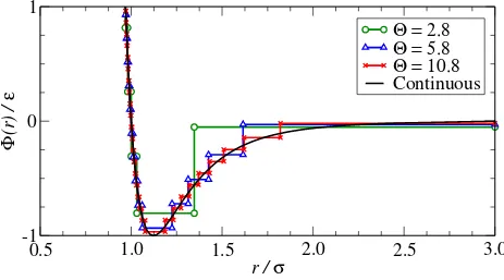
[image:3.612.72.535.73.330.2]Continuous
FIG. 1. A comparison of the continuous Lennard-Jones potential (solid) and three stepped ap-proximations created using Eq. (4) for step placement and Eq. (11) for the step energies.
potentials (e.g., GROMACS12 and ESPResSo13). This is even more surprising given that
the very first particle simulations were carried out using a discrete potential1, almost ten
years before Verlet’s simulations.
It is only relatively recently that fine-tuned discrete potentials for detailed, atomistic
simulations have started to appear; these include force fields for a broad range of compounds,
including hydrocarbons14 and fluorocarbons15, organic acids16, esters, ketones and other
organic compounds17,18, phospholipids19, and peptides and proteins20. The use of TPT has
even allowed rapid and direct fitting of discrete potentials to experimental data10,14,20,21. In
addition, standard simulation packages for event-driven molecular dynamics have also begun
to appear22.
The strong theoretical frameworks and stable simulation algorithm makes discrete
po-tentials an attractive alternative to continuous popo-tentials.
Complex discontinuous potentials are typically reported as a table of discontinuity
loca-tions and energies23. Although these two classes of potentials are distinct, it is clear that
they may be made equivalent, provided a sufficient number of discontinuities or steps are
dis-continuities for an accurate representation of a continuous potential is not well understood
and is the subject of this paper.
It is desirable to have a mechanism to convert continuous potentials to discrete forms.
This mapping must be optimized in the sense that it uses the smallest number of
discontinu-ities to reduce the complexity of the converted potential and to minimize the computational
cost of simulation. Chapela et al.23 was the first to attempt to represent the continuous
Lennard-Jones potential by an equivalent discrete form. This mapping was optimized “by
hand” to reproduce the thermodynamic properties at one state point, but more recent
work24–27 has focused on using regular stepping to automate the conversion process.
Con-tinuous potentials have also been used to directly specify the location of discontinuities8
allowing a convenient implementation of asymmetric potentials in event-driven dynamics;
however, the optimization of this conversion is yet to be explored. Recently, there has been
an attempt to replace the soft interactions of continuous potentials entirely with collision
dynamics at low densities28 but this approach is restricted to low density systems.
In this work, the mapping of a continuous potential to a discrete form is investigated
using the Lennard-Jones potential. In the following section, the placement of discontinuities
and allocation of step energies is discussed before the methods are evaluated in Sec. III. The
most efficient mapping scheme is then evaluated for a range of thermodynamic and transport
properties in Sec. IV. A comparison between time-stepping and event-driven simulation is
performed in Sec. V. Finally, the conclusions of the paper are presented in Sec. VI.
II. DISCRETIZATION OF THE POTENTIAL
The primary aim of this work is to develop an algorithm to convert a continuous
po-tential to an optimal discrete form: one that provides an accurate approximation of the
original continuous potential and can be simulated at a minimal computational cost. As the
computational cost of an event-driven simulation is roughly proportional to the number of
discontinuities encountered by the particles, it is vital that the number of discontinuities or
steps used to achieve a set level of accuracy is minimized.
The location of a single step i in a spherically-symmetric discrete potential is specified
by the segment [ri+1, ri] between the ith and i+ 1th discontinuities. The discontinuities,
simplification made in this work is to require that each step is directly representative of the
segment of the continuous potential lying within the same limits [ri+1, ri]. This allows the
task of discretizing the potential to be split into two smaller tasks: the optimal placement
of discontinuities and the determination of an effective step energy for a segment of the
continuous potential.
It is common to accelerate molecular dynamics calculations by truncating the interaction
potential at a cut-off radiusrcutoff, thus requiring only local particle pairings to be considered
in force calculations. Typically in time-stepping simulations, the potential is also shifted to
eliminate the discontinuity at the cutoff in order to avoid the presence of impulsive forces.
For example, the truncated, shifted Lennard-Jones potential is given by
Φ(r) =
ΦLJ(r)−ΦLJ(r
cutoff) if r≤rcutoff
0 if r > rcutoff
. (1)
As each step of the discontinuous potential represents a segment of the original continuous
potential, the first discontinuity is defined to lie at the cutoff radius (i.e. r1 =rcutoff), while
all other discontinuities lie within in the region r ∈ (0, rcutoff). It is tempting to also define
an inner hard-core radius of the stepped potential using one of the available methods (e.g.,
see Ref. 29); however, this would require each step energy to somehow compensate for
the overly repulsive core, inextricably linking step placement and energy once again. The
available methods for placing discontinuities are reviewed in the next section before the
algorithms used to generate representative step energies are discussed.
A. Location of Discontinuities
The simplest approach to place the discontinuities of a discrete potential is to divide the
region r∈(0, rcutoff) into a number of steps of equal width ∆r25.
ri,∆r =rcutoff−(i−1)∆r (2)
The total number of discontinuities/steps in the potential (including the cutoff) is given by
brcutoff/∆rc+ 1.
It is not immediately clear that a uniform radial placement of the steps is the natural
each step of the potential. In this case, each step location is determined using the following
recursive expression
ri,∆v =
r3i−1,∆v− 3 ∆v
4π 1/3
(3)
The total number of discontinuities in the potential is then b4π r3
cutoff/3 ∆vc+ 1.
The primary disadvantage of the approaches outlined above is that they do not attempt
to adapt the step locations according to the behavior of the potential. It is likely that the
performance of both algorithms is particularly sensitive to the configuration of the steps
near the minimum of the potential where the interaction energy changes rapidly.
It has also been proposed8,27to discretize continuous potentials by placing discontinuities
at fixed intervals of interaction energy ∆Φ. This approach allows a controlled resolution
of the potential, while balancing the contribution of each step and allows a straightforward
extension to asymmetric potentials. The locations of the discontinuities are the ordered
solutions to the following set of equations
Φ(r) =j∆Φ j ∈Z (4)
The application of Eq. (4) to the shifted, truncated Lennard-Jones potential results in an
infinite number of steps due to the singularity at r = 0. In practice, the high-energy steps
are inaccessible and only a small number need to be computed during the simulation.
Before these approaches can be evaluated, a technique for determining the step energies
must be selected. This is discussed in the following section.
B. Step Energy
With the location of each step defined through one of the above algorithms, an algorithm
for determining the effective energy of a segment of the potential is required. In the limit of
a large number of discontinuities/small segments, the original continuous potential must be
recovered. Chapela et al.25 have evaluated three approaches based on point sampling of the
continuous potential.
ΦLef ti = Φ (ri+1) (5)
ΦM idi = Φ
ri+ri+1 2
(6)
where Φi is the energy of step i over the region [ri+1, ri] of the discontinuous potential.
Chapela et al.25 report that mid-point sampling (ΦM id
i ) of the underlying continuous
poten-tial is the most effective at reproducing the original behavior of the Lennard-Jones potenpoten-tial,
whereas left sampling is more appropriate for the Yukawa potential. It is easy to define
other methods of point sampling, such as the minimum edge energy used by van Zon and
Schofield8. A straightforward choice is to sample the potential at the distance which divides
the step into two equal volumes.
ΦM id V oli = Φ
r3
i +ri3+1 2
1/3!
. (8)
It is also possible to define alternative approaches which do not rely on point-sampling,
such as an equal area approach27; however, it is more desirable to directly match the
ther-modynamic properties of the converted potentials. Unfortunately, matching properties, such
as the pressure, would require the use of an accurate free energy, which is typically
unavail-able. Successful attempts have been made to adjust stepped potentials to directly match
the predictions of the TPT to experimental data for a range of thermodynamic properties26;
however, the resulting equation of state is still approximate and the expressions are rather
complicated. In this work, the focus is on directly reproducing the properties of the
con-tinuous potential system. One simple approach is to use the lowest order density correction
to both the pressure and free-energy, given by the second virial coefficient, which is directly
calculated from the interaction potential. The contribution of a segment of the potential to
the second virial may be calculated as follows
B2(ri, ri+1, T) = −2π
Z ri
ri+1
e−βΦ(r)−1r2dr (9)
where β = 1/(kBT), T is the absolute temperature of the system, and kB is the Boltzmann
constant. The energy of the step can then be set to match the contribution to the
sec-ond virial coefficient for the correspsec-onding segment of the continuous potential, using the
following expression
Φviriali (T) = −kBT ln
3
r3
i −r3i+1
Z ri
ri+1
r2e−βΦ(r)dr
. (10)
Application of this algorithm leads to excellent agreement at low densities for the pressure;
however, the algorithm has a cumbersome dependence on the temperature, which may not
equating the virial contribution reduces to taking a volume average of the energy within a
step:
ΦV olumei = 3
r3
i −ri3+1
Z ri
ri+1
Φ (r)r2dr. (11)
This indicates that the volume averaged approach will also yield a good reproduction of
the pressure near the ideal gas limit of high-temperature and low-density. It should be
noted that both virial and volume-averaging approaches will set an infinite energy for the
innermost step of the Lennard-Jones potential due to the singularity at r = 0. This can
have a dramatic effect on the potential as the step placement algorithms in Eqs. (3) and (4)
use a finite number of steps to represent the repulsive core.
III. COMPARISON OF MAPPING PROCEDURES
To compare the various methods for mapping potentials, molecular dynamics simulations
of N = 1372 discontinuous and continuous Lennard-Jones particles with rcutoff = 3σ were
performed over a range of densities, ρ =N/V, and temperatures, kBT. To collect
thermo-dynamic properties, each simulation was run for 20 (mσ2/ε)1/2 for equilibration before five
production runs of 30 (mσ2/ε)1/2 were used to collect averages and obtain estimates of the
uncertainty. Dynamical properties were collected using three runs, each 103(mσ2/ε)1/2in
du-ration. Averages are reported here with error bars corresponding to the standard deviation
between runs. Simulations for the continuous truncated, shifted Lennard-Jones potential
were performed using the ESPResSo13 package with a time step of 0.002 (mσ2/ε)1/2 and a
Langevin thermostat with a friction parameter of 1 (ε/mσ2)1/2. Discrete potential
simula-tions were performed using the DynamO22 package with an Andersen thermostat controlled
to 5% of the overall events. During the collection of dynamical properties, the thermostat is
disabled after the equilibration period and the temperature is monitored to ensure it remains
within 2% of the set value.
The mapping procedures must be evaluated on a basis of accuracy as a function of
computational cost. As event-driven simulators process events at a constant rate, the
com-putational cost is proportional to the number of events that must be processed per unit of
simulation time. Each additional discontinuity within the potential will generate additional
by the number of discontinuities in the well of the potential. A straightforward parameter for
the order of approximation of the potential, Θ, can then be defined for each step placement
algorithm as follows:
Θ = 1 +
(rcutoff−rmin)/∆r for Eq. (2)
4π r3cutoff−r3min/3 ∆v for Eq. (3)
−Φ(rmin)/∆Φ for Eq. (4)
where rmin = 21/6σ is the location of the minimum of the Lennard-Jones potential. The
parameter Θ is continuous, and as Θ → ∞, the continuous Lennard-Jones potential is
re-covered. The integer part of Θ corresponds to the number of discontinuities in the attractive
section of the potential and at whole integer values of Θ, a discontinuity is placed at the
minimum of the potential.
A. Placement of the discontinuities
The methods for placing the discontinuities of a discrete potential (Eq. (2)–(4)) are
eval-uated first. An example comparison of the calculated pressure and internal energy for a
high-density super-critical state point using the mid-point sampling algorithm (Eq. (6)) to
set the step energies is given in Fig. 2. A temperature of kBT /ε = 1.3 is used in these
simulations as it is well-above the critical temperature kBTc/ε ≈ 1.15 of the rcutoff = 3σ
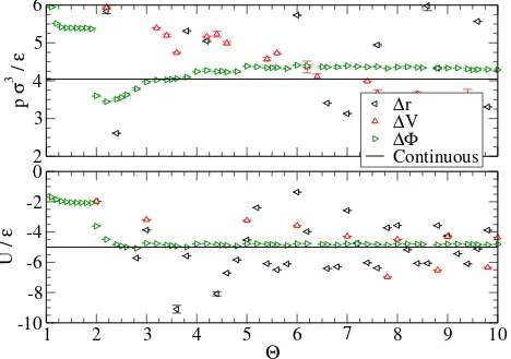
system30 to avoid entering the two-phase region. It is clear from this comparison alone that
the algorithm using fixed energy intervals (∆Φ, Eq. (4)) is superior to the other approaches.
The algorithm demonstrates rapid convergence to the result obtained from the continuous
potential simulations once Θ >2, and allows a controlled approximation of the continuous
potential. The slight offset in the pressure at higher values of Θ is later shown to be an
artifact of using the mid-point sampling method for the step energy. The radial placement
algorithm (Eq. (2), ∆r) appears to converge towards the continuous potential result for the
internal energy but requires a large number of steps and its performance is erratic. The
radial and volumetric placement algorithms are particularly sensitive to the order of
ap-proximation. For example, the volumetric algorithm is only accurate for the internal energy
at integer values of Θ which correspond to a discontinuity placed at the minimum of the
potential. This highlights the importance of a good approximation of the potential in this
2
3
4
5
6
p
σ
3
/
ε
∆
r
∆
V
∆Φ
Continuous
1
2
3
4
5
6
7
8
9
10
Θ
-10
-8
-6
-4
-2
0
U /
[image:10.612.73.541.74.403.2]ε
FIG. 2. Pressure,p, and internal energy,U, for a super-critical LJ liquid (kBT /ε= 1.3,ρσ3 = 0.85) as a function of the number of attractive steps, Θ, in the potential. The solid line indicates the continuous potential result. Each set of data points correspond to a different algorithm for placing the steps whereas the Φmidi algorithm is used to set the step energy in all cases.
Further simulations have been carried out using all step-energy algorithms over a range
of densities and temperatures and are in qualitative agreement with the trends outlined
in Fig. 2; therefore, it is clear that the fixed energy interval algorithm given in Eq. (4) is
the most appropriate as it is the only approach which allows a controlled approximation of
the stepped potential. A full review of the available step energy algorithms using the fixed
B. Step energy
The algorithms for setting the step energy, given in Eqs. (5)–(11), are evaluated by
comparing predictions for the pressure (see Fig. 3) and internal energy (see Fig. 4) for two
super-critical state-points at low and high density. Equation (4) is used to specify the step
locations and the order of approximation is again controlled by specifying the number of
discontinuities Θ in the attractive section of the potential. To confirm that Θ is the correct
basis for comparison of these algorithms, the simulation event rates as a function of Θ are
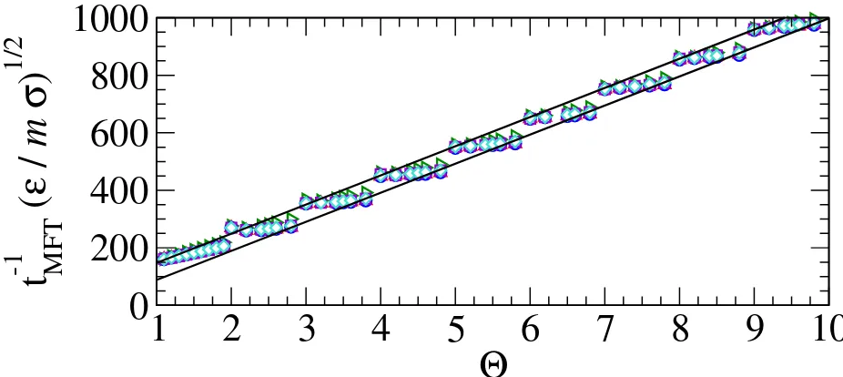
presented in Fig. 5. Each step-energy algorithm has an almost identical cost as a function of
Θ and, for Θ>2, a remarkable linear correlation is observed between the rate of events. As
the event-driven simulation algorithm processes events at an approximately constant rate for
a given cutoff and density, this demonstrates that there is a direct correspondence between
Θ and the computational cost, making it a suitable basis for comparison.
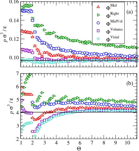
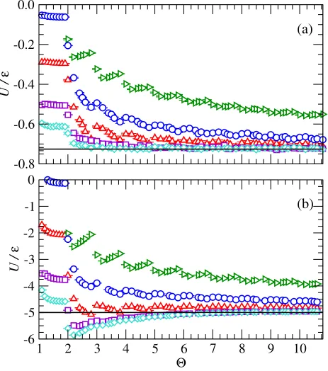
At low densities, equating the virial contributions provides an excellent agreement for
the pressure for all orders of approximation (see Fig. 3a), as expected. This is particularly
interesting as for Θ ∈ (1,2) the discontinuous potential is a core-softened square-well
po-tential. For predictions of the internal energy, the virial approach performs well only once
a step is added between the minimum and the cutoff (Θ>2 in Fig. 4a). The results of the
Left sampling algorithm are not visible in the figures as they appear to enter the two-phase
region, resulting in a very poor approximation. The Left, Mid, and Right algorithms display
a strong dependence on the step placement through large changes near integer values of Θ.
The relatively smooth dependence of the Volume, and Virial algorithms on the Θ parameter
indicates that these approaches provide a relatively unbiased sampling of the underlying
potential. The MidVol algorithm performs worse overall than the Mid-point sampling
ap-proach and the Volume averaging algorithm performs almost as well as the Virial algorithm.
The Volume algorithm appears to be a suitable replacement for the Virial if the temperature
is not known and provided Θ >1. At high densities (see Figs. 3b and 4b), the Virial and
Volume averaging approaches still perform well but surprisingly the Mid-point sampling
out-performs all other techniques for 1<Θ <4. This is likely due to a fortuitous cancellation
of errors rather than an inherent advantage of the method, as its performance worsens for
higher order approximations (Θ>4). It is clear that an excellent approximation is obtained
1
2
3
4
5
6
7
8
9
10
Θ
2
3
4
5
6
7
p
σ
3
/
ε
0.10
0.12
0.14
0.16
p
σ
3
/
ε
Φ
Mid
Φ
Right
Φ
MidVol
Φ
Volume
Φ
Virial
(a)
[image:12.612.73.538.75.579.2](b)
FIG. 3. A comparison of the stepped potential predictions for the pressure, p, of a kBT /ε = 1.3 Lennard-Jones fluid as a function of attractive step count Θ at (a) low (ρσ3 = 0.1) and (b) high (ρσ3 = 0.85) densities. The solid line indicates the continuous potential result and each
Overall, setting the step energy through a volume average of the energy of the underlying
continuous potential appears to yield a good approximation, provided Θ>1. The additional
complexity of a temperature-dependent potential through using the Virial approach does not
appear justified at these conditions unless Θ<1, but the reproduction of the internal energy
is unacceptable at such a low order of approximation. Although it might be expected that the
temperature dependence will become increasingly important at lower temperatures, further
simulations carried out in the liquid branch atkBT /ε= 0.85 and ρσ3 = 0.85 yielded similar
results to those reported, indicating the temperature correction is unjustified even when well
within the liquid phase.
In summary, the placement of discontinuities using Eq. (4) and allocation of their energies
using Eq. (11) appears to provide the best approximation of the continuous Lennard-Jones
potential of the methods examined for the evaluated state points. As the computational
cost primarily depends on the integer portion of Θ (see Fig. 5), it is optimal to select values
of Θ with large fractional parts, such as Θ≈5.8.
IV. OPTIMAL ALGORITHM EVALUATION
The conversion algorithm which yielded the best performance, given in Eq. (4) and
Eq. (11), is now fully evaluated across a wide range of state points. In particular, the
trade-off between accuracy of reproduction and computational cost is explored. All values
of Θ have a fractional part of .8 due to the step-wise scaling of the computational cost with
Θ (see Fig. 5).
A. Thermodynamic Properties
To validate the thermodynamic properties of the system, the phase diagram (see Fig. 6)
and vapor pressures (see Fig. 7) are calculated using Monte Carlo simulations in the grand
canonical ensemble, using multi-canonical sampling to overcome the free energy barrier
between the liquid and vapor phases31–33. The simulations were performed in a cubic box of
side length 7σ. Approximately 100×106 configurations were sampled at each temperature,
with 50% attempted displacement moves and 50% attempted particle insertion/deletion
used to determine the multi-canonical weights at the lower temperatures. The coexistence
point at each temperature was determined by adjusting the chemical potential to equate the
areas of the density histogram corresponding to the liquid and vapor phase.
The critical point is estimated by using a least-squares fit of the critical scaling of the
density difference and the law of rectlinear diameters
ρL−ρV =C1
1− T Tc
βc
(12)
1
2(ρL+ρV) =ρc+C2(T −Tc) (13)
where ρL and ρV are the liquid and vapor densities at a temperature of T, and Tc and ρc
are the critical properties which, along with C1 to C2, are fitting parameters. A critical
exponent of βc= 0.3265 is used here. The optimal conversion procedure appears to deliver
a smooth convergence to the continuous potential result for the phase envelope in Fig. 6,
highlighting the value of Θ as an order of approximation. The Θ = 10.8 system closely
reproduces the thermodynamic behavior of the continuous Lennard-Jones potential, with
only a slight under-estimation of the liquid transition density for low-temperature liquids.
For values of Θ = 3.8 and 5.8, the approximation is remarkably close for such a low order
approximation but for Θ = 2.8, the approximation rapidly deteriorates. Given the relatively
low values of Θ, the potential appears to be performing well when compared to previous
conversions23,25,27, although direct comparisons are difficult due to different choices for the
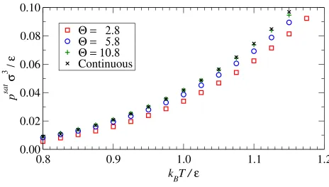
cutoff radius. Results for the vapor pressures in Fig. 7 confirm the close reproduction of the
continuous potential phase diagram for the Θ = 10.8 system.
Although the discrete approximations appear to converge to the thermodynamic
prop-erties of the Lennard-Jones fluid, there are subtle differences in the microscopic structure.
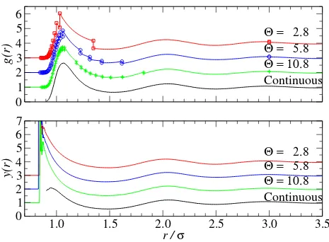
The discontinuities in the energetic potential lead to discontinuities in g(r), as illustrated
for a high-density state point in Fig. 8. For low-order approximations the differences are
sig-nificant, but for Θ = 10.8 the g(r) is closely reproduced. The continuous cavity distribution
function, defined as y(r) = g(r)eβΦ(r), yields a close agreement between all approximations
(see Fig. 8b). The sampling of y(r) is poor for the continuous potential near r → 0.9 as
the g(r) is low in this region; however, the use of the event-rate formulas allows a higher
accuracy of sampling in this region for the stepped potential which explains the discrepancy.
Despit these small differences in micro-structure, the overall thermodynamic properties of
B. Dynamical Properties
To fully validate the effectiveness of the conversion process, a number of dynamical
prop-erties have been calculated and are compared against the reference simulation results of
Meier et al.35–37, and Bugel and Galliero38. Dynamical properties are difficult to calculate
accurately as they require long simulation times to allow hydrodynamic behavior to appear.
The literature values used here have been obtained using larger cut-offs (in the range of
rcutoff/σ = 5 to 6, depending on density). This will only cause small deviations except
near the critical point of the literature fluid (kBTc/ε ≈ 1.34) which is above that of the
rcutoff/σ = 3 fluid used here (kBTc/ε ≈ 1.17). Density sweeps are performed at two
su-percritical temperatures, kBT /ε= 1.35 near to the critical point of the reference data and
kBT /ε = 2.5. Relative error estimates are obtained by combining the standard deviation
between simulation runs for both the reference and discontinuous results.
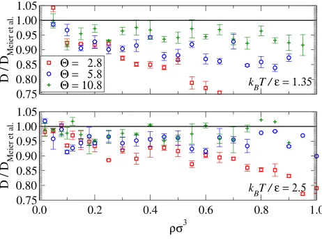
Results for the self-diffusion coefficient are presented in Fig. 9. It is clear that dynamical
properties such as the diffusion coefficient are much more difficult to approximate when
compared with the thermodynamic properties. Low-order approximations have a reduced
diffusion coefficient when compared to the continuous potential. This effect is due to the
difference in critical temperatures which results in an lower reduced temperature for the
low-order approximations in the theorem of corresponding-states. The results for Θ = 10.8
are acceptable with a maximum deviation of ≈8% over both isotherms.
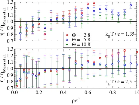
Results for the viscosity are presented in Fig. 10. The Θ = 10.8 results are within 10% of
the continuous results for both isotherms, except at the lowest two densities. The
disagree-ment at low densities is likely due to the increased proportion of glancing interactions which
shifts the emphasis from a close reproduction of the well to the outer tail of the potential. It
may be that regular stepping of the potential using radial or volumetric placement is more
suitable at very low gas densities. Overall, agreement is good given the uncertainty in the
results.
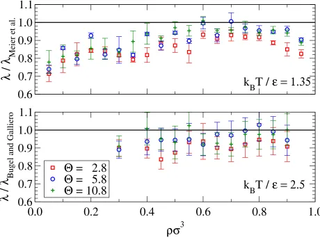
Results for the thermal conductivity are presented in Fig. 11. Agreement is good for high
temperatures but for the kBT /ε = 1.35 isotherm the stepped approximations significantly
underestimate the thermal conductivity of the continuous potential. The disagreement at
low-density may again be caused by an increase in glancing interactions but the discrepancy
conductivity with cutoff range there is an enhancement of the thermal conductivity in region
of the critical point38. As the literature values at this temperature are near the critical point
the stepped potential results will slightly under predict the thermal conductivity. For liquid
densities (ρ σ3 & 0.6), the stepped approximation satisfactorily reproduces the continuous potential behavior.
V. COMPUTATIONAL COST
Using the selected conversion procedure, the computational cost of stepped/event-driven
and continuous/time-stepping techniques can be compared on an equal basis. The relative
speed of each method, defined as the simulation time processed per unit of CPU time, for
a kBT /ε= 1.3 isotherm is presented in Fig. 12. It is immediately apparent that the use of
event-driven methods is only advantageous at gas densities (ρ σ3 .0.02) or below, where it significantly outperforms time stepping methods. Hybrid time-stepping/event-driven
meth-ods also display this dramatic increase in performance at low densities39 as the system
dynamics becomes dominated by two-particle collisions. The use of stepped potentials will
eliminate some of the overhead of hybrid techniques which indicates promising future
ap-plications of the potentials developed here in rarefied gas flow simulation. The comparison
carried out here is only for serial execution performance; however, parallel algorithms for
event-driven simulation exhibit good scaling40 and will be evaluated in future.
VI. CONCLUSIONS
In this work, we have examined several methods for mapping a continuous interaction
potential to a discrete, stepped potential. These methods were compared on their ability of
the resulting discrete potential to reproduce the thermodynamic and transport properties of
the continuous potential system over a broad range of conditions. Of the various methods
which were examined to locate the discontinuities of the potential, the best was found to be
at fixed intervals of energy. Setting the step energy through a volume average of the energy
of the underlying continuous potential appears to give the a good overall approximation
provided Θ>1 and an excellent approximation for Θ = 10.8.
stepped potential approximation were compared on the basis of their processing rates for a
unit of simulation time. Stepped Lennard-Jones potentials are increasingly efficient when
compared to continuous forms at gas densities or lower (ρ σ3 .0.02 which is around 33 kg/m3 for Argon). This indicates the potentials here may be used to significantly accelerate
simu-lations of shock waves39 or other complex rarefied gas systems where DSMC techniques are
currently applied.
Short range or repulsive potentials, such as the Weeks-Chandler-Anderson potential,
should prove far more efficient targets for conversion given the speed of hard-sphere
simula-tions. The Hertz potential, used in simulations of solids particles, is particularly interesting
as the stepped equivalent may be arbitrarily steep. This, combined with the analytical
dynamics of the event-driven technique, will allow the stable and efficient use of realistic
materials parameters in granular simulations. The only obstacle to this application is the
conversion of the dissipative inter-particle forces which will be explored in a future
publica-tion.
VII. ACKNOWLEDGMENTS
The authors would like to acknowledge the support of the Maxwell compute cluster funded
by the University of Aberdeen.
REFERENCES
1B. J. Alder and T. E. Wainwright, J. Chem. Phys. 27, 1208 (1957).
2T. P¨oschel and T. Schwager, Computational Granular Dynamics (Springer, New York,
2005).
3R. A. Gingold and J. J. Monaghan, Mon. Not. R. Astron. Soc. 181, 375 (1977).
4L. Verlet, Phys. Rev. 159, 98 (1967).
5J. Ponder and D. Case, Adv. Prot. Chem. 66, 27 (2003).
6A. MacKerel Jr., C. Brooks III, L. Nilsson, B. Roux, Y. Won, and M. Karplus, in The
Encyclopedia of Computational Chemistry, Vol. 1, edited by P. von R. Schleyer (John
7J. M. Haile, Molecular Dynamics Simulation - Elementary Methods (Wiley-Interscience,
New York, 1997).
8R. van Zon and J. Schofield, J. Chem. Phys. 128, 154119 (2008).
9J. A. Barker and D. Henderson, J. Chem. Phys. 47, 2856 (1967).
10O. Unlu, N. H. Gray, Z. N. Gerek, and J. R. Elliott, Ind. Eng. Chem. Res. 43, 1788
(2004).
11S. Chapman and T. G. Cowling,The Mathematical Theory of Non-uniform Gases, 3rd ed.
(Cambridge Mathematical Library, 1991).
12D. Van der Spoel, E. Lindahl, B. Hess, G. Groenhof, A. E. Mark, and H. J. C. Berendsen,
J. Comput. Chem. 26, 1701 (2005).
13H.-J. Limbach, A. Arnold, B. A. Mann, and C. Holm, Comput. Phys. Commun. 174, 704
(2006).
14J. Cui and J. J. Richard Elliott, J. Chem. Phys. 116, 8625 (2002).
15A. D. Sans and J. R. Elliott, Fluid Phase Equilib. 263, 182 (2008).
16A. Vahid, A. D. Sans, and J. R. Elliott, Ind. Eng. Chem. Res. 47, 7955 (2008).
17F. S. Baskaya, N. H. Gray, Z. N. Gerek, and J. R. Elliott, Fluid Phase Equilib. 236, 42
(2005).
18A. M. Hassan, D. T. Vu, D. A. Bernard-Brunel, J. R. Elliott, D. J. Miller, and C. T. Lira,
Ind. Eng. Chem. Res. 51, 3209 (2012).
19E. M. Curtis and C. K. Hall, J. Phys. Chem. B 117, 5019 (2013).
20H. D. Nguyen and C. K. Hall, Biophys. J. 87, 4122 (2004).
21M. C. dos Ramos, H. Docherty, F. J. Blas, and A. Galindo, Fluid Phase Equilib. 276,
116 (2009).
22M. N. Bannerman, R. Sargant, and L. Lue, J. Comput. Chem. 32, 3329 (2011).
23G. Chapela, L. E. Scriven, and H. T. Davis, J. Chem. Phys. 91, 4307 (1989).
24J. Torres-Arenas, L. A. Cervantes, A. L. Benavides, G. A. Chapela, and F. del Rio, J.
Chem. Phys. 132, 034501 (2010).
25G. A. Chapela, F. del Rio, A. L. Denavides, and J. Alejandre, J. Chem. Phys.133, 234107
(2010).
26S. Ucyigitler, M. C. Camurdan, and J. R. Elliott, Ind. Eng. Chem. Res. 51, 6219 (2012).
27G. A. Chapela, F. del Rio, and J. Alejandre, J. Chem. Phys. 138, 054507 (2013).
29J. A. Barker and D. Henderson, J. Chem. Phys. 47, 4714 (1967).
30B. Smit, J. Chem. Phys. 96, 8639 (1992).
31N. B. Wilding, Phys. Rev. E 52, 602 (1995).
32G. Orkoulas and A. Z. Panagiotopoulos, J. Chem. Phys. 110, 1581 (1999).
33N. B. Wilding, Am. J. Phys. 69, 1147 (2001).
34M. N. Bannerman and L. Lue, J. Chem. Phys. 133, 124506 (2010).
35K. Meier, Computer simulation and interpretation of the transport coefficients of the
Lennard-Jones model fluid, Ph.D. thesis, Dept. Mech. Eng., Uni. Fed. Armed forces,
Ham-burg (2002).
36K. Meie, A. Laesecke, and S. Kabelac, J. Chem. Phys. 121, 3671 (2004).
37K. Meie, A. Laesecke, and S. Kabelac, J. Chem. Phys. 121, 9526 (2004).
38M. Bugel and G. Galliero, Chem. Phys. 352, 249 (2009).
39P. Valentini and T. E. Schwartzentruber, J. Comput. Phys. 228, 8766 (2009).
1
2
3
4
5
6
7
8
9
10
Θ
-6
-5
-4
-3
-2
-1
0
U /
ε
-0.8
-0.6
-0.4
-0.2
0.0
U /
ε
(a)
[image:20.612.75.538.74.598.2](b)
1
2
3
4
5
6
7
8
9
10
Θ
0
200
400
600
800
1000
t
-1
MFT
(
ε
/
m
σ
)
[image:21.612.71.534.71.278.2] [image:21.612.73.536.416.680.2]1/2
FIG. 5. The events per particle per unit of simulation time, given by t−M F T1 = 2Nevents/(N tsim) whereNeventsis the number of events caused by a particle pair encountering a discontinuity during a simulation of durationtsim, for various step placement algorithms at a temperature ofkBT /ε= 1.3 and density of ρσ3 = 0.85. The symbols are described in Fig. 3 and the straight lines have been regressed to the virial data points for Θ>2 with fractional parts of .0 and .8.
0.0
0.2
0.4
0.6
0.8
ρσ
30.8
0.9
1.0
1.1
1.2
1.3
k
BT /
ε
Θ = 2.8
Θ = 3.8
Θ = 5.8
Θ = 10.8
Continuous
FIG. 6. Phase diagram of the rcutoff = 3σ Lennard-Jones fluid. Symbols denote MCMC results
0.8
0.9
1.0
1.1
1.2
k
B
T /
ε
0.00
0.02
0.04
0.06
0.08
0.10
p
sat
σ
3
/ ε
Θ = 2.8
Θ = 5.8
Θ = 10.8
[image:22.612.70.534.68.331.2]Continuous
0
1
2
3
4
5
6
g(r)
1.0
1.5
2.0
2.5
3.0
3.5
r /
σ
0
1
2
3
4
5
6
7
y(r)
Θ = 2.8
Θ = 5.8
Θ = 10.8
Continuous
Θ = 2.8
Θ = 5.8
Θ = 10.8
[image:23.612.71.536.64.406.2]Continuous
0.0
0.2
0.4
0.6
0.8
1.0
ρσ
30.75
0.80
0.85
0.90
0.95
1.00
1.05
D / D
Meier et al.
0.75
0.80
0.85
0.90
0.95
1.00
1.05
D / D
Meier et al.
Θ = 2.8
Θ = 5.8
Θ = 10.8
k
BT /
ε = 1.35
k
B
T /
ε = 2.5
[image:24.612.73.535.71.418.2]0.7
0.8
0.9
1.0
1.1
1.2
1.3
η
/
η
Meier et al.0.0
0.2
0.4
0.6
0.8
1.0
ρσ
30.7
0.8
0.9
1.0
1.1
1.2
1.3
η
/
η
Meier et al.Θ
= 2.8
Θ
= 5.8
Θ
= 10.8
k
B
T /
ε = 1.35
k
[image:25.612.74.534.72.420.2]B
T /
ε = 2.5
0.6
0.7
0.8
0.9
1.0
1.1
λ
/
λ
Meier et al.0.0
0.2
0.4
0.6
0.8
1.0
ρσ
30.6
0.7
0.8
0.9
1.0
1.1
λ
/
λ
Bugel and GallieroΘ
= 2.8
Θ
= 5.8
Θ
= 10.8
k
BT /
ε = 1.35
[image:26.612.74.534.72.420.2]k
BT /
ε = 2.5
0.0
0.1
0.2
0.3
0.4
0.5
0.6
0.7
ρσ
310
-110
010
110
2TS / ED (speed)
Θ = 2.8
Θ = 5.8
Θ = 10.8
FIG. 12. The relative calculation-speed (simulation time processed per unit of CPU time) of time-stepping (TS) and event-driven (ED) molecular dynamics for a Lennard-Jones isotherm at
[image:27.612.73.534.75.348.2]