Visually driven analysis of movement data by progressive clustering

City, University of London Institutional Repository

Citation

:

Andrienko, G. (2008). Visually driven analysis of movement data by progressive clustering. Information Visualization, 7(3-4), pp. 225-239. doi: 10.1057/palgrave.ivs.9500183

This is the unspecified version of the paper.

This version of the publication may differ from the final published

version.

Permanent repository link:

Link to published version

:

Copyright and reuse:

City Research Online aims to make research

outputs of City, University of London available to a wider audience.

Copyright and Moral Rights remain with the author(s) and/or copyright

holders. URLs from City Research Online may be freely distributed and

linked to.

Visually–driven analysis of movement data by progressive

clustering

Salvatore Rinzivillo* Dino Pedreschi Mirco Nanni Fosca Giannotti

KDD Lab, University of Pisa {rinziv,pedre}@di.unipi.it

KDD Lab, ISTI – CNR, Pisa {mirco.nanni,fosca.giannotti}@isti.cnr.it

Natalia Andrienko Gennady Andrienko

Fraunhofer Institute IAIS, Sankt Augustin, Germany {gennady.andrienko, natalia.andrienko}@iais.fraunhofer.de

Abstract

The paper investigates the possibilities of using clustering techniques in visual exploration and analysis of large numbers of trajectories, i.e. sequences of time-stamped locations of some moving entities. Trajectories are complex spatio-temporal constructs characterized by diverse non-trivial properties. To assess the degree of (dis)similarity between trajectories, specific methods (distance functions) are required. A single distance function accounting for all properties of trajectories, first, is difficult to build, second, would require much time to compute, third, might be difficult to understand and to use. We suggest the procedure of progressive clustering where a simple distance function with a clear meaning is applied on each step, which leads to easily interpretable outcomes. Successive application of several different functions enables sophisticated analyses through gradual refinement of earlier obtained results. Besides the advantages from the sense-making perspective, progressive clustering enables a rational work organization where time-consuming computations are applied to relatively small potentially interesting subsets obtained by means of “cheap” distance functions producing quick results. We introduce the concept of progressive clustering by an example of analyzing a large real dataset. We also review the existing clustering methods, describe the method OPTICS suitable for progressive clustering of trajectories, and briefly present several distance functions for trajectories.

Keywords: trajectories, spatio-temporal data, visual analytics, geovisualization, exploratory data analysis, scalable methods.

1

Motivation

The large amounts of movement data collected by means of current tracking technologies such as GPS and RFID call for scalable software techniques helping to extract valuable information from these masses. This has stimulated active research in the fields of geographic information science (Hornsby & Egenhofer 2002, Miller 2005), databases (Güting & Schneider 2005), and data mining (Giannotti & Pedreschi, 2007). A general framework for analysis of movement data where database operations and computational methods are combined with interactive visual techniques is suggested in (Andrienko et al. 2007). Among other methods, the framework includes cluster analysis, which is the primary focus of this paper.

use certain methods for estimating differences between objects in terms of relevant characteristics. These differences are also called “distances” (in the abstract space of the characteristics) and the methods for computing them are called “distance functions”.

It should be noted that clustering is not a standalone method of analysis whose outcomes can be immediately used for whatever purposes (e.g. decision making). An essential part of the analysis is interpretation of the clusters by a human analyst; only in this way they acquire meaning and value. To enable the interpretation, the results of clustering need to be appropriately presented to the analyst. Visual and interactive techniques play here a key role. Clustering methods are often included in visualization systems and toolkits (e.g. Seo & Shneiderman 2002, Guo et al. 2006, Sips et al. 2007, Schreck et al. 2007).

In analysis of movement data, the objects that need to be analyzed are trajectories, i.e. sequences of time-stamped locations of some moving entities. These are quite complex spatio-temporal constructs. Their potentially relevant characteristics include the geometric shape of the path, its position in space, the life span, and the dynamics, i.e. the way in which the spatial location, speed, direction and other point-related attributes of the movement change over time. Clustering of trajectories requires appropriate distance functions which could properly deal with these by no means trivial properties. However, creating a single function accounting for all properties is hardly a reasonable endeavor irrespective of the effort this would require. On the one hand, not all characteristics of trajectories may be simultaneously relevant in practical analysis tasks. On the other hand, clusters produced by means of such a universal function would be very difficult to interpret.

A more reasonable approach is to give the analyst a set of relatively simple distance functions dealing with different properties of trajectories and provide the possibility to combine them in the process of analysis. The simplest and most intuitive way is to do the analysis in a sequence of steps. In each step, clustering with a single distance function is applied either to the whole set of trajectories or to one or more of the clusters obtained in the preceding steps. If it is clear to the analyst how each distance function works (of course, the analyst needs to know only the principle but not the technical details), the clusters obtained in each step are easy to interpret by tracking the history of their derivation. Step by step, the analyst progressively refines his/her understanding of the data. New analytical questions arise as an outcome of the previous analysis and determine the further steps. The whole process is called “progressive clustering”. Visual and interactive techniques are essential for supporting this process.

Besides the ease of interpretation, there is one more reason for the progressive way of clustering. The properties of trajectories differ in their complexity; hence, the corresponding distance functions will inevitably require different amounts of computational resources. Applying a sophisticated distance function to a large dataset may take much time and result in undesirable gaps in the process of analysis. It may be more reasonable first to divide the dataset into suitable parts by means of “cheaper” functions and apply more demanding functions to the parts of the data.

2

Background

2.1 Clustering 

As we have mentioned, the aim of a clustering method is to produce a set of groups of objects where the objects in the same group (cluster) are near each other and the groups are distant from each other. The problem of finding the optimal clustering is NP-hard. There are several strategies proposed in the literature for finding a near-optimal solution in polynomial time: partition-based, hierarchical, and density-based algorithms (Kaufman & Rousseeuw, 1990).

The partition-based methods, as suggested by the name, partition the dataset into sub-groups, such that the objective function for each cluster is maximized. In order to reach a good approximation, the partitions are refined in an iterative way until the result converges to a stable solution. This approach is used, for example, in k-means and k-medoid methods, like the CLARANS method proposed in (Ng & Han, 1994): given an input parameter k, the method chooses k random objects from the datasets as cluster seeds and assigns all the other ones to the nearest seed. Then, the algorithm refines the clusters by moving objects from one cluster to another until a stable configuration is reached. The algorithm of Self-Organizing Map (Kohonen 2001), or SOM, has a similar principle of work. First, a two-dimensional matrix of prototype vectors is built either randomly or by applying the Principal Component Analysis to the data (at the end, each vector will represent a cluster). Then, for each object, the closest prototype vector is found. The vector and its neighbors in the matrix are adjusted to this object using the technique of neural network training. This operation is done iteratively; the duration of the training is specified as a parameter. SOM combines clustering and projection and is therefore popular among researchers designing tools for visual data analysis (e.g. Guo et al. 2006, Schreck et al. 2007). The partition-based methods produce convex clusters as a result of adding objects to the nearest clusters.

The hierarchical approaches work through an iterative hierarchical decomposition of the dataset, represented by means of a dendrogram. This is a tree-like representation of the dataset where each internal node represents a cluster and the leaves contain the single objects of the dataset. A dendrogram may be created either from the bottom (objects are grouped together) or from the top (the dataset is split into parts until a termination condition is satisfied).

The density-based clustering methods rely on the concept of density to identify a cluster: for each point inside a cluster, the neighborhood of a given radius has to contain at least a given minimum number of points, i.e. the density of the cluster has to be not less than the density threshold. Density-based algorithms are naturally robust to such problems as noise and outliers since they usually do not affect the overall density of the data. Trajectory data often suffer from some underling random component and/or low resolution of the measurements, so noise tolerance is a highly desirable feature.

2.2 OPTICS 

In this section we briefly present the OPTICS algorithm and the underlying definitions, specifically, of a core object and the reachability distance of an object p with respect to a predecessor object o.

An object p is called a core object if the neighborhood around it is a dense region, and therefore p should belong so some cluster and not to the noise. Formally:

Definition 1 (Core Object): Let p be an object in a dataset D, Eps a distance threshold, and NEps(p) the Eps-neighborhood of p (i.e. the set of objects {x in D | d(p,x) < Eps}). Given an

integer parameter MinNbs (minimum number of neighbors), p is a core object if NEps(p) >=

MinNbs.

Using the core object definition, we can distinguish the objects that are potentially in some clusters from the noise. However, the problem of assigning each object to an appropriate cluster remains. The OPTICS method proceeds by exploring the dataset and enumerating all the objects. For each object p it checks if the core object conditions are satisfied and, in the positive case, starts to enlarge the potential cluster by checking the condition for all neighbors of p. If the object p is not a core object, the scanning process continues with the next unvisited object of D. All objects that lie on the border of a cluster may not satisfy the core object condition, but this does not prevent them to be included in a cluster. In fact, a cluster is determined both by its core objects and the objects that are reachable from a core object, i.e. the objects that do not satisfy the core object condition but that are contained in the Eps-neighborhood of a core object. From these considerations, we have the following:

Definition 2 (Reachability Distance): Let p be and object, o a core object, Eps a distance threshold and NEps(o) the Eps-neighborhood of o. Denoting with n-distance(p) the distance

from p to its n-th neighbor in the order of proximity, and given an integer parameter MinNbs, the reachability distance of p with respect to o is defined as: reach-dEps,MinNbs(p,o) =

max{MinNbs-distance(o), d(o,p)}. The distance denoted as MinNbs-distance(o) is also called the core distance of o.

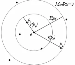
The reachability distance of p with respect to o is essentially the distance between the two objects except for the case when p is too close. In this case, the distance is normalized to the core distance. The concepts are illustrated in Figure 1.

Figure 1. An illustration of the definitions 1 and 2 by points: the point o is a core point since in its neighborhood of radius Eps there are at least 3 points (MinNbs=3). The core distance of the point o is given by the distance to its third neighbor in the order of proximity (the smaller circle). The reachability distance of the point p1 denoted as r(p1) is equal to the core distance.

The reachability distance of the point p2, denoted r(p2), is equal to the distance from o to p2.

the next object pi chosen from D is the object with the smallest reachability distance with

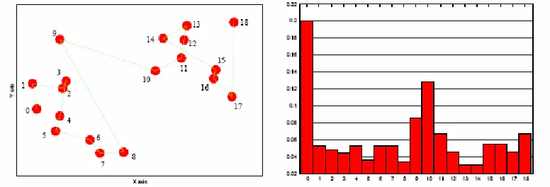
respect to all already visited core objects. The process is repeated until all objects in D have been considered. The results are summarized in a reachability plot: the objects are represented along the horizontal axis in the order of visiting them and the vertical dimension represents their reachability distances.

Figure 2. An example of reachability plot. On the left, the order of visiting the objects (points) is indicated by numbers.

Intuitively, the reachability distance of an object pi corresponds to the minimum distance from

the set of its predecessors pj, 0<j<i. As a consequence, a high value of the reachability

distance roughly means a high distance from the other objects, i.e. indicates that the object is in a sparse area. Clusters appear in the reachability plot as valleys; thus, in Figure 2 two clusters may be detected. To partition the data into a set of clusters plus noise, it is now sufficient to choose a threshold value Eps for the maximum value of reachability distance allowed within a cluster. The peaks that exceed this value are considered as noise and the valleys below this value as clusters.

Ankerst et al. (1999) have demonstrated that the shape of the reachability plot is insensitive to the choice of the value for the parameter Eps. Essentially, this parameter only affects the separation of the noise from the clusters: a low value results in treating less dense regions as noise while a high value would turn them into (parts of) clusters.

Furthermore, the result of the OPTICS algorithm is also insensitive to the original order of the objects in the dataset. The objects are visited in this order only until a core object is found. After that, the neighborhood of the core object is expanded by adding all density-connected objects. The order of visiting these objects depends on the distances between them and not on their order in the dataset. It is also not important which of density-connected objects will be chosen as the first core object since the algorithm guarantees that all the objects will be put close together in the resulting ordering. A formal proof of this property of the algorithm is given in (Ester et al. 1996).

reasonable to use different values of MinNbs for different subsets of the data. We shall return to this issue in describing the exploration of the example dataset.

Figure 3. The impact of the parameter MinNbs. Top: MinNbs=5; bottom: MinNbs=20.

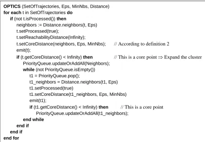
Figure 4 presents the pseudo code of the OPTICS implementation. Among the other parameters, the method takes as an input also the distance function. This function determines the distance between two trajectories and the neighborhood of a given trajectory.

Figure 4. A pseudo code of the OPTICS algorithm.

OPTICS (SetOfTrajectories, Eps, MinNbs, Distance)

for each t in SetOfTrajectories do

if (not t.isProcessed()) then

neighbors := Distance.neighbors(t, Eps) t.setProcessed(true);

t.setReachabilityDistance(Infinity);

t.setCoreDistance(neighbors, Eps, MinNbs); // According to definition 2

emit(t);

if (t.getCoreDistance() < Infinity) then // This is a core point ⇒ Expand the cluster

PriorityQueue.updateOrAddAll(Neighbors);

while (not PriorityQueue.isEmpty())

t1 = PriorityQueue.pop();

t1_neighbors = Distance.neighbors(t1, Eps)

t1.setProcessed(true)

t1.setCoreDistance(t1_neighbors, Eps, MinNbs)

emit(t1);

if (t1.getCoreDistance() < Infinity) then // This is a core point

PriorityQueue.updateOrAddAll(t1_neighbors);

end while

end if

end if

The complexity of the algorithm is O(n× log n) where n is the number of the objects in the dataset and log n is the time for selecting the neighborhood of each object. It is assumed that there is an index of objects that allows retrieving the neighborhood of an object in logarithmic time. In our prototype implementation, however, we use a linear scan of the dataset to select the neighborhood of an object. This increases the complexity of the implementation to n2. This is acceptable for the purpose of our experimentation, but we are working on devising various methods of indexing to decrease this complexity. Building an index of trajectories is, in general, not a simple task since each distance function requires its own indexing strategy. However, for basic distance functions, the definition of an index may be quite simple. This can be aptly used in progressive clustering, in which simpler distance functions are more likely to be applied in earlier steps to the whole data or large subsets. With the use of appropriate indexes, these steps can be done more efficiently. More complex functions can then be applied in successive steps of the analysis to much smaller subsets, so that the use of indexes is no longer so critical.

3

Clustering

of

trajectories

Spatio-temporal data introduce new dimensions and novel issues in performing the clustering task. In movement data, for a given object id we have a triple (xi,yi,ti) for each time instant ti.

The set of triples for a given object id may be viewed as a function fid: time → space, which

assigns a spatial location to the object id for each time moment. We call such a function a trajectory and we concentrate on the problem of clustering a given set of trajectories.

The extensions of existing clustering methods to the spatio-temporal domain can be classified into two approaches: feature-based models and direct geometric models (Kriegel et al. 2003). In the first case, the objects of the dataset are projected to a multidimensional vector space and their similarities are computed in the new projection. In the second model, the spatial and temporal characteristics of the objects are directly used for defining the distances. We follow the second approach by developing a library of distance functions that compare the trajectories according to various spatial and spatio-temporal properties an analyst may be interested to consider. The properties include the origins of the trips, the destinations, the start and end times, the routes (where a route is characterized in terms of the geometric shape of the footprint and its spatial position and orientation), and the dynamics of the movement (which may be defined in terms of the relative times when different positions have been reached and/or the variation of the speed throughout the trip).

The distance functions accounting for these properties differ in complexity. Thus, very simple functions are sufficient for comparing trajectories according to the origins and/or destinations. The functions “common source” and “common destination” compute the distances in space between the starting points or between the ending points of trajectories, respectively. These are the distances on the Earth surface if the positions are specified in geographical coordinates (latitudes and longitudes) or the Euclidean distances otherwise. The function “common source and destination” returns the average of the distances between the starting points and between the ending points of two trajectories. In a similar way, temporal distances between the starting and/or between the ending moments of trajectories are used to compare and group trajectories according to the absolute times of the trips.

spatial distances between the corresponding points. The functions differ in the way of choosing the check points. In the function “k points”, the user specifies the desired number (k) of check points, which are selected so as to keep the number of intermediate points between them constant. In the function “time steps”, the user specifies the desired temporal distance between the check points. Both functions roughly estimate the similarity of the routes; the precision depends on the number of check points. The latter function also estimates the similarity of the movement dynamics. It should be noted that these two functions can work sufficiently well only for “perfect” data, i.e. complete trajectories with equal time intervals between the position records and only minor positioning errors. Unfortunately, this is not always the case.

A more complex distance function “route similarity” has been designed to tolerate incomplete trajectories (i.e. where some parts in the beginning and/or in the end are missing) and more significant positioning errors. It is also better suited to unequal time intervals between records. The function repeatedly searches for the closest pair of positions in the two trajectories. It computes the mean distance between the correspondent positions along with a penalty distance for the unmatched positions. A detailed description of the function is presented in (Andrienko et al. 2007).

The function “route similarity + dynamics” takes into account the relative times of arriving in corresponding positions. The relative times are the temporal distances to some reference time moments, which are individual for each trajectory. These may be, for example, the starting times of the trajectories or their ending times. In our implementation, the reference time moments in two trajectories under comparison are defined by the spatially closest pair of their positions, i.e. the times of arriving in these positions are taken as the reference times. This particular way of selecting reference times has been chosen for the purpose of tolerance to possible incompleteness of trajectories.

After the reference times of two trajectories have been selected, the further comparison is done as follows. Let us denote the trajectories as P and Q and their reference times as t0(P) and t0(Q), respectively. We scan all the points of P starting from the position p0 visited at the time t0(P). For each position pi, we search for the point qi in Q such that the time distance of qi from t0(Q) is the closest among all positions to the time distance of pi from t0(P). The distance between P and Q is computed as the average sum of the distances between the corresponding positions plus penalties in case of different durations of the two trajectories. The same approach can be easily applied for considering the absolute times of the two trajectories. In this case, corresponding positions of two trajectories are the positions achieved at the same or possibly closest time moments. In both relative and absolute time strategies, two approaches to the selection of corresponding points are possible: selection from the existing sample points registered by the positioning device and interpolation of positions between the sample points.

The library of distance functions is easily extendable. In particular, it is possible to add functions accounting for various auxiliary information such as properties of the moving individuals (age, profession, …), type of movement (walking, biking, driving, …), or properties of the environment (types of roads, land cover, points of interest, …). It is also possible to use a pre-computed matrix of pairwise distances between trajectories coming from an external source.

functions taking into account the absolute times of the trips are not relevant since the data refer to quite a short time interval of four hours. Third, the functions comparing dynamics are useful mostly for trajectories with similar routes. As will be further seen, route similarity occurs relatively rarely in the example dataset.

Our selection of the functions for the example analysis scenario will allow us to demonstrate a reasonable way of combining simple and complex distance functions in exploring a big dataset. The general strategy is to apply simpler and therefore less time-consuming functions for dividing the data into manageable subsets with clear semantics and to use more sophisticated and resource-demanding functions for in-depth exploration of the subsets.

4

Visualization

of

clusters

of

trajectories

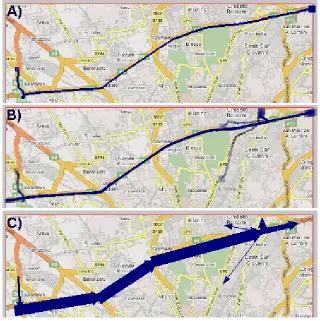
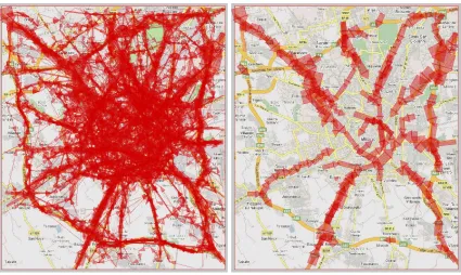
To visualize a trajectory on a map display, we draw a polygonal line connecting its successive positions. The starting position is marked by a small hollow square and the ending position by a larger filled square (Figure 5A). Trajectories can also be visualized in a space-time cube where the vertical dimension represents time. However, when multiple trajectories are visualized in this way, both the map and the cube get severely cluttered and therefore illegible. A possible approach to solving this problem is based on clustering. The idea is to group trajectories by similarity using clustering techniques (Figure 5B) and then represent each group in a summarized way without drawing the individual trajectories (Figure 5C).

A representation like in Figure 5C is built by counting the numbers of moves between significant places passed by the trajectories. The significant places may include road crossings and various areas of interest. The widths of the directed lines are proportional to the numbers of moves. Thick lines indicate the major flows while thin lines represent deviations.

However, it is quite problematic to make this approach work for arbitrary movement data. One of the problems is that so coherent trajectories as in Figure 5B occur very rarely in real data while most trajectories are quite dissimilar to others. Another problem is that significant places are often not known. Besides these difficulties, the approach itself is insufficient as is deals only with the spatial properties of trajectories but not with the temporal properties.

While the best possible solution to all problems is yet to be found, we have developed a workable approach which helps to cope with complexities of real data. The approach is based on dynamic aggregation of movement data. A dynamic aggregator is a special kind of object which is linked to several other objects (members of an aggregate) and computes certain aggregate attributes such as the member count and the minimum, maximum, average, median, etc. from the attribute values of the members. The aggregator reacts to various kinds of interactive filtering by adjusting the values of the aggregate attributes: only the members that pass through the current filter are taken into account in computing the values.

We have introduced two types of dynamic aggregators of movement data: summation places and aggregate moves. A summation place is an area in space which is “aware” of all trajectories passing through it and stores the positions and times of entering in the area and exiting from it. The fragments of the trajectories lying inside the area are the members of the place. A summation place counts its members and computes such aggregate attributes as the minimum, maximum, average, median, and total time spent in the area, statistics of the speeds, etc., as well as the number of starts (first points of trajectories) and the number of ends (last points). An aggregate move is defined by two places A and B and is “aware” of all trajectories that visit A and B in this specific order without passing any intermediate place. The members of the move are the respective trajectory fragments. An aggregate move produces the count of its members and statistical summaries of the lengths of the fragments, their durations, and speeds.

A summation place may optionally be visualized on a map by drawing the outline of the area and/or filling the interior. Irrespective of whether the places themselves are shown or not, current values of selected aggregate attributes may be visualized by graduated symbols or by diagrams. An aggregate move is visualized on a map as a vector (directed line) as shown in Figure 5C. The thickness of the vector is proportional to the current value of the member count (default) or any other aggregate attribute selected by the user.

The interactive filters, which make dynamic aggregates re-compute their attribute values, include temporal filter (selection of a time interval), spatial filter (selection of a “window” in space), attribute filter (selection of trajectories by their attributes such as duration and length), and cluster filter (selection of clusters). In re-computing, the aggregates take into account only the active members, i.e. the members that have passed through all currently set filters. When an aggregate move has no active members, it does not appear on a map; otherwise, the thickness of the corresponding vector is adjusted to the current value of the currently represented aggregate attribute. The same happens to symbols or diagrams representing aggregate attributes of summation places.

can additionally apply the temporal filter for exploring the time-related properties of the trajectories in the cluster.

A crucial prerequisite for creating dynamic aggregators of movement data is the availability of a set of significant places, which can be turned into summation places and determine the possible aggregate moves. As already mentioned, significant places are often not known in advance. Therefore, we have developed a method for obtaining a kind of “surrogates” of significant places. The method, first, extracts characteristic points from the available trajectories, which include the start and end points, the points of turns and the points of stops. For determining the turns and stops, the method requires two user-specified thresholds: the minimum angle of a turn and the minimum duration of a stop, i.e. keeping the same position. Then, the method builds areas (for simplicity, circles) around concentrations of characteristic points and around isolated points. The sizes of the areas depend on the user-defined minimum and maximum circle radii. These areas then serve as surrogate significant places for building dynamic aggregates of the movement data.

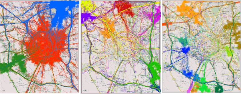
It should be noted that the use of computationally produced surrogates may not give so nice and clear picture of summarized trajectories as by using semantically defined significant places. The difference can be seen by comparing Figures 5C and 6C.

Figure 6 demonstrates a typical result of applying our method to a big dataset with very high variation among the trajectories. For such data, the method produces a large number of rather chaotically distributed circles. As is seen in Figure 6A, the circles passed by a cluster of trajectories may not be suitably aligned (in contrast, for producing Figure 5C, we have manually defined significant places by encircling the road crossings on the background map image). This produces excessive aggregate moves, which obscure the view. Note that the summarization works well enough in the regions where the circles are adequately aligned.

It is clear that further work is required for finding a proper way for automated extraction of significant places from movement data. It may seem that applying the method described above separately to each cluster of trajectories rather than to the whole dataset might solve the problem. However, not always clusters consist of coherent trajectories; counter-examples may be seen in Figure 9.

To alleviate the problem and understand better the properties of clusters of trajectories, an analyst may use additional visual and interactive facilities. Thus, interactive filtering applied to aggregate moves (rather than to the original trajectories) allows the analyst to disregard minor variations and uncover major flows pertaining to a cluster of trajectories (Figure 7). It may also be helpful to visualize the aggregate attributes associated with the summation places. For example, the pie charts in Figure 8 (left) represent the numbers of starts (yellow segments) and ends (blue segments) of trajectories in automatically extracted summation places. To avoid or reduce overlapping between the symbols or diagrams representing the attributes, it may be reasonable to summarize movement data also by cells of a regular grid (Figure 8, right). An additional advantage of this is the equal sizes of the summation places, which facilitates comparisons between the respective aggregate characteristics.

Figure 8. Visualization of aggregate attributes in summation places.

In the example analysis scenario, which follows, we shall use illustrations where clusters are visualized by coloring trajectory lines; no aggregation is applied. The reason is that the illustrations have to be static while the aggregation techniques are dynamic and work sufficiently well only in combination with the facilities for interaction.

5

Example:

progressive

clustering

of

car

trajectories

in

Milan

5.1 Data 

For the example analysis scenario we use a subset of a dataset collected by GPS-tracking of 17,241 cars in Milan (Italy) during one week from Sunday to Saturday. The subset consists of 6187 trajectories made on Wednesday 04/04/2007 between 6:00AM and 10:00AM. The reason for selecting a subset is that the clustering techniques are not yet mature enough to cope with the whole dataset, which includes about 176,000 trajectories. However, even this relatively small subset is too big for analyzing by purely visual and interactive techniques and is therefore sufficient for studying the potential for using clustering in visual exploration of movement data. In our study, we use our implementation of the algorithm OPTICS. It has three parameters: the distance threshold Eps and the minimum number of neighbors MinNbs, according to Definition 1, plus the distance function F. Some of the distance functions may have additional parameters.

5.2 Progressive clustering for handling uneven data density 

adjusted to the density of the data. However, the data may not be equally dense throughout the whole space. This is the case for the Milan dataset.

Progressive clustering is a good practical approach to analyzing unevenly dense data. The idea works as follows. At the beginning, clustering with a large value for MinNbs is applied to the whole dataset. The analyst should “play” with the parameter until getting a few clusters that are spatially coherent and well interpretable. In addition to these, many small clusters can be produced but the analyst may ignore them on this stage. After examining, describing, and explaining the most significant clusters, the analyst excludes their members from the further analysis and applies clustering with smaller MinNbs to the remaining data. Again, the goal is to obtain coherent and interpretable clusters. Then, as on the previous stage, the largest clusters are examined, described, and excluded from the further consideration. After that, the procedure may be repeated for the remaining data with yet smaller MinNbs. If the remaining data are sparse, it may also be meaningful to increase the value of Eps. Note that one and the same distance function is used on each stage of the exploration and only the parameter values vary. The procedure is repeated until the analyst gets a sufficiently complete and clear understanding of the dataset properties related to the chosen distance function.

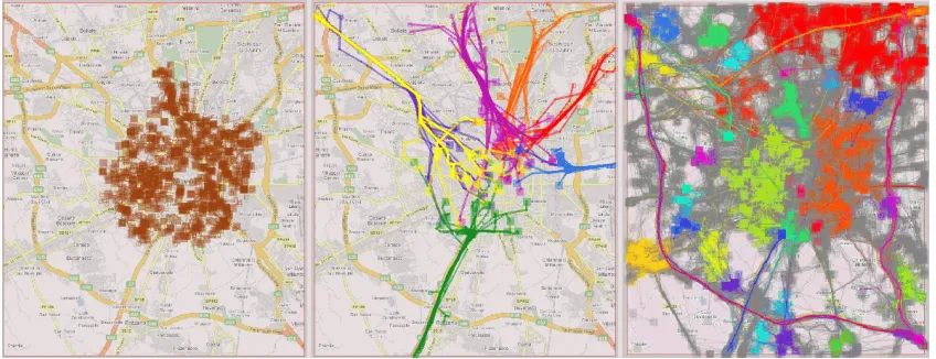
Figure 9. Progressive clustering helps to detect coherent clusters in data with uneven spatial density.

Figure 9 presents the results of three steps of progressive clustering according to trip destinations (i.e. end points of the trajectories) we have applied to the subset of trajectories under analysis. The trajectories are drawn on the map display with 30% opacity (the degree of opacity may be interactively changed, as well as the line thickness). The map on the left represents 3 biggest clusters resulting from the clustering with F=”common destination”, Eps=500m and MinNbs=15: 1781 trajectories in the “red”, 893 in the “blue” and 354 in the “green” cluster; all other clusters are much smaller. We can clearly distinguish the trajectories ending in the city center from those ending on the northeast and southwest. Before coming to this result, we tried to cluster the same trajectories with Eps=500m and MinNbs=10. The attempt was not successful, i.e. no understandable clusters were obtained. In particular, all the trajectories visible on the left of Figure 9 and many others were put together.

The sizes of the orange and brown clusters are 219 and 207, respectively, and the sizes of the other clusters range from 91 to 45. Besides these, there are many much smaller clusters, which are not very interesting.

In this way, we have identified the major regions to which people drive in the morning of a working day. Progressive clustering with the use of the same distance function but different parameter settings has helped us to cope with uneven spatial density of the data. However, for gaining a comprehensive view of the data, it is insufficient to use just one simple distance function but is necessary to combine several functions, as will be demonstrated in the next subsection.

5.3 Progressive clustering for deeper understanding of data 

The clustering with the use of the distance function “common destination” allowed us to group the trajectories according to the trip destinations. One of our findings is that many trips end in the center of Milan (the red cluster in Figure 9 left). Now we are interested in exploring these trips more in depth. We select the “red” cluster and apply further clustering with the distance function “route similarity” to its member trajectories. This allows us to detect that a great part of them are very short trajectories within the center. The image on the left of Figure 10 presents the biggest cluster obtained with Eps=1000 and MinNbs=5. It consists of 517 short trajectories situated inside the center; this is 29% of all trajectories ending in the center. Among the remaining trajectories, there are rather few clusters of trajectories with similar routes, and the clusters are very small. The biggest of them are shown in the middle of Figure 10; the sizes range from 11 to 28 (the line thickness has been increased for a better visibility). 1074 trajectories, i.e. 63% of 1781, have been classified as “noise”, which means the absence of frequent routes among them.

Figure 10. Left and middle: the major clusters obtained by applying the distance function “route similarity” to the trajectories ending in the center of Milan. Right: a result of clustering all trajectories with the distance function “common source and destination”.

than the function “route similarity” while being adequate to our goal. The results of the clustering made with the parameters Eps=800m and MinNbs=8 are presented on the right of Figure 10. They show that in most cases when trajectories have close starts and close ends the starts are also close to the ends. Thus, the clusters where the starts of the trajectories significantly differ from their ends include in total only 127 trajectories (2%) whereas the clusters where the starts are close to the ends include 1439 trajectories, or 23% of all (4621 trajectories, or 75%, have been regarded as “noise”; they are shown in grey). It can be noted that the clusters include not only very short trajectories but also long trajectories where the car drivers returned to the starting points of the trips. However, these long trajectories are much less numerous than the short ones. The results obtained with the parameters Eps=800m and MinNbs=8 are consistent with results obtained using other parameter values.

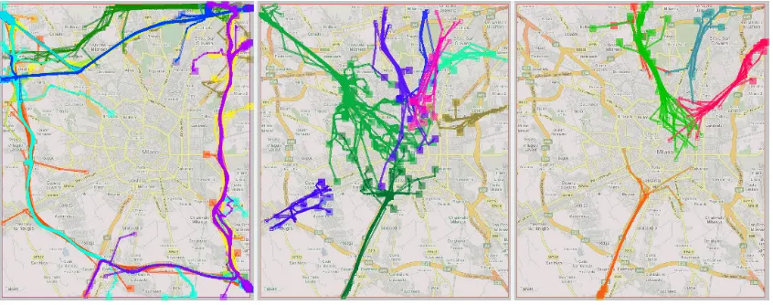
Hence, about a quarter of the trajectories represent trips where the starts are close to the ends, and most of them are short local trips. Now we want to investigate the properties of the trips on longer distances. In particular, we are interested in typical (frequently taken) routes. We exclude the clusters with the local and round trips and apply clustering with the distance function “route similarity” to the remaining trajectories, including the “noise”. Figure 11 presents the results of the clustering with the parameters Eps=800m and MinNbs=5. The biggest cluster (bright green lines in the middle image) consists of 66 trajectories, the remaining 40 clusters contain from 5 to 25 trajectories, and 4163 trajectories have been classified as “noise”. Among the trajectories included in the clusters there are three major types of routes: (1) peripheral routes using the belt around the city (Figure 11 left); (2) radial routes from the periphery towards the inner city (Figure 11 middle); (3) radial routes from the inner city towards the periphery (Figure 11 right). It may be seen that the clusters of inward routes (middle) are bigger and more numerous than the clusters of outward routes (right). This may signify that inward movement occurs more frequently than outward movement in the morning of a working day. Interestingly, there are no frequent inward routes from the south-east.

Figure 11. Results of clustering of the trajectories with the starts differing from the ends using the function “route similarity”. Left: peripheral routes; middle: inward routes; right: outward routes.

6

Discussion

6.1 Summary of findings 

Our exploration of the trajectories made by 5063 different cars in Milan in the morning of Wednesday, 04/04/2007, have brought us the following findings:

1) The destinations of the trips are spread throughout the territory. There are no places significantly more popular than the others.

2) A large part of the trips are small local trips where the starts are close to the ends.

3) There is a large variety of routes. Groups of trajectories following similar routes are very small in comparison to the size of the dataset. Most trajectories follow quite unique routes.

4) Among the relatively frequent routes, there are many peripheral routes using different segments of the road belt around the city. The trajectories following these routes mostly do not enter the inner city.

5) Relatively frequent are also radial routes from the periphery inside the city. The most frequent is the route from the north-west.

6) Outward trips are less frequent than inward trips and there are fewer re-occurring routes among them.

The findings have been obtained by means of clustering combined with interactive visual tools. Of course, clustering could also be used in combination with other tools, but we intentionally avoided this in our example exploration to keep consistency with the focus of this paper.

6.2 Roles of clustering and visualization 

It is important to stress that obtaining clusters is not the goal but the means of the exploration. The goal is to gain knowledge about the data and the phenomenon they represent. Therefore, the findings listed above are the main results of our work while the clusters are used for substantiating and illustrating these results.

The clustering can fulfill its role only in combination with appropriate visualization, which, in particular, shows the relationships between the clusters and additional spatial information, which is provided by the background map. This allows the analyst to interpret the clusters, i.e. attach meaning to them and derive knowledge.

6.3 Novelty 

The idea of progressive clustering appears very simple and obvious. Therefore, it seems very unlikely that it has not been used elsewhere yet. Indeed, similar concepts of “stepwise clustering” and “subspace clustering” exist in data mining. The approaches suggested so far can be grouped into two categories: optimization-oriented refinement and result tuning. The approaches from the first group optimize the algorithm performance by, for example, providing approximated query results, which are later refined only for the borderline cases (Brecheisen et al. 2006), or by pre-computing rough clusters, which are then refined through more sophisticated aggregations (Breunig et al. 2001). The approaches from the second group allow the user to tune clustering outcomes to his/her background knowledge. They are based on visually-aided interactive post-processing, e.g. by moving objects between clusters (Assent et al. 2007, Nam et al. 2007).

objects with heterogeneous properties (spatial, temporal, numeric, and qualitative), which cannot be handled in the same way. The idea is to use a different distance function for each kind of property for allowing the analyst to gradually build a comprehensive understanding of the set of objects. To the best of our knowledge, this idea has not been introduced in the literature yet. The possible reason is that clustering techniques have been mostly devised for objects represented as points in a multi-dimensional space where all dimensions are treated in the same way. When it comes to complex spatio-temporal constructs such as trajectories, this approach cannot be quite adequate any more.

In principle, it is possible to combine several distance functions accounting for diverse properties in a single function, which could account for all properties simultaneously. However, this involves two serious disadvantages. First, such a hybrid function would be very expensive in terms of computational resources. It would not be reasonable to apply it directly to an entire big dataset since it may turn out that only a part if it really requires a detailed analysis. Second, the results of such clustering would be very difficult to understand since the clusters would simultaneously differ in many diverse respects. Therefore, the progressive approach appears more practical and usable.

6.4 Sensitivity issues 

Progressive clustering is an iterative procedure where results of clustering are used for selection of a subset of data to be examined through further clustering with a different distance function or different parameters. The procedure is not linear but involves returns to previous steps and selection of different subsets for further examination. The process could be viewed as a branching tree (there are systems where analysis sessions can be explicitly visualized in this way, e.g. Goodell et al. 2006).

Of course, the order in which different distance functions or different parameter settings are applied has a dramatic effect on the clusters appearing at the end of a branch. However, this “instability” should not be regarded as a weakness of the method. First, as we have noted earlier, clustering is primarily an instrument for gaining knowledge; hence, the knowledge acquired on each step is a much more important result of analysis than the particular clusters coming at the end. Second, a reasonable order of applying distance functions and parameter settings is often prescribed by the nature and properties of the data and the analysis tasks. Third, for some combinations of distance functions there is a logical order of application. Thus, it is reasonable to apply the functions grouping trajectories by their starts and/or ends before the function grouping trajectories by the routes.

has a limited scalability with respect to the number of clustered objects and is quite demanding in terms of user’s workload. Hence, the problem of comparison of clustering results requires further research.

Another possibility could be automated tuning of clustering parameters. The key issue here is automatic assessment of the quality or interestingness of clusters, which could direct an optimization procedure towards the best possible results. There are some generic quality measures such as cohesion and separation (Tan et al. 2005) or average density (Nanni & Pedreschi 2006). However, such mathematical properties of clusters do not necessarily correlate with semantic interpretability or interestingness. Especially for such complex objects as trajectories, automated evaluation of clusters is an open problem.

6.5 Progressive clustering versus hierarchical clustering 

One of the possible ways of using progressive clustering is top-down hierarchical partitioning of the original dataset, when the user chooses each time one cluster and subdivides it through further clustering. However, the user is neither limited to this approach nor encouraged to proceed in this particular way. The user can select any number of previously derived clusters to form a subset of objects for further analysis. For example, the user could unite all clusters of inward trips shown in Figure 11 and further cluster these trips according to their temporal characteristics. It is even possible to “mix” clusters resulting from different runs of the clustering tool, although this requires a few additional interactive operations. Hence, the cluster structure which may be derived by progressive clustering is, generally, a lattice; a hierarchy is only a special case. The procedure is flexible enough to fit to various user needs and specifics of real data.

7

Conclusion

Trajectories of moving objects are complex spatio-temporal constructs, and analysis of multiple trajectories is a challenging task. To help a human analyst to make sense from large amounts of movement data, we suggest the procedure of progressive clustering supported by visualization and interaction techniques. A good property of this procedure is that a simple distance function with a clear principle of work can be applied on each step, which leads to easily interpretable outcomes. However, successive application of several different functions enables sophisticated analyses through gradual refinement of earlier obtained results. Besides the advantages from the sense-making perspective, progressive clustering provides a convenient mechanism for user control over the work of the computational tools as the user can selectively direct the computational power to potentially interesting portions of data instead of processing all data in a uniform way. In particular, the analyst may use “expensive” (in terms of required computer resources) distance functions for relatively small potentially interesting subsets obtained by means of “cheap” functions producing quick results. In the future, we plan to extend the ideas of progressive clustering to analysis of extremely large datasets that cannot be processes in the main memory of the computer. The general approach is that clustering is applied to a sample of trajectories, and then computations in the database are used to attach remaining trajectories to the clusters obtained. This approach requires efficient algorithms for checking trajectory membership in a cluster.

Acknowledgments

We are grateful to the reviewers of our paper for their recommendations for improving the text and suggestion of interesting questions for further research work.

References

Andrienko, G., Andrienko, N., & Wrobel, S. (2007). Visual Analytics Tools for Analysis of Movement Data. ACM SIGKDD Explorations , 9(2), December 2007, 38-46.

Ankerst, M., Breunig, M., Kriegel, H.-P., & Sander, J. (1999). OPTICS: Ordering Points to Identify the Clustering Structure. Proceedings of ACM SIGMOD International Conference on Management of Data (SIGMOD'99). Philadelphia: ACM, 49-60

Assent, I., Krieger, R., Müller, E., & Seidl, T. (2007). VISA: visual subspace clustering analysis. ACM SIGKDD Explorations, 9(2), December 2007, 5-12

Brecheisen, S., Kriegel, H.-P., & Pfeifle, M. (2006). Multi-step density-based clustering. Knowledge and Information Systems, 9(3), March 2006, 284-308

Breunig, M.M., Kriegel, H.-P., Kröger, P., & Sander, J. (2001). Data bubbles: quality preserving performance boosting for hierarchical clustering. Proceedings of the 2001 ACM SIGMOD international conference on Management of data, Santa Barbara, California, USA, 79-90

Ester, M., Kriegel, H.-P., Sander, J., & Xu, X. (1996). A density-based algorithm for discovering clusters in large spatial databases with noise. Second International Conference on Knowledge Discovery and Data Mining, Portland, Oregon, 226-231

Giannotti, F., & Pedreschi, D., eds. (2007). Mobility, Data Mining and Privacy - Geographic Knowledge discovery. Springer, Berlin.

Goodell, H., Chiang, C.-H., Kelleher, C., Baumann, A., & Grinstein, G. (2006). Collecting and harnessing rich session histories, Proceedings of the International Conference on International Conference on Information Visualization (IV’06), London, July 5-7, 117-123.

Guo, D., Chen, J., MacEachren, A.M., & Liao, K. (2006). A Visualization System for Spatio-Temporal and Multivariate Patterns (VIS-STAMP), IEEE Transactions on Visualization and Computer Graphics, 12(6), 1461-1474

Güting, R., & Schneider, M. (2005). Moving Objects Databases. Elsevier

Hornsby, K., Egenhofer, M.J. (2002). Modeling moving objects over multiple granularities. Annals of Mathematics and Artificial Intelligence, 36, 177-194.

Kaufman, L., & Rousseeuw, P. (1990). Finding Groups in Data: an Introduction to Cluster Analysis. John Wiley & Sons.

Kohonen, T. (2001). Self-Organizing Maps. Springer, Berlin, 3rd edition.

Kriegel, H., Brecheisen, S., Kroeger, P., Pfeifle, M., & Schubert, M. (2003). Using sets of feature vectors for similarity search on voxelized CAD objects. SIGMOD Conference, 587-598

Miller, H.J. (2005), A Measurement Theory for Time Geography, Geographical Analysis, 37, 17–45

Nanni, M., & Pedreschi, D. (2006). Time-focused clustering of trajectories of moving objects. Journal Intelligent Information Systems, 27, 267-289.

Ng, R., & Han, J. (1994). Efficient and Effective Clustering Methods of Spatial Data Mining. Proc. 20th Int. Conf. on Very Large Data Bases. Santiago, Chile.

Pelekis, N., Kopanakis, I., Marketos, G., Ntoutsi, I., Andrienko, G., & Theodoridis, Y. (2007) Similarity search in trajectory databases. In Proc. 14th Int. Symposium Temporal Representation and Reasoning (TIME 2007), IEEE Computer Society Press, 2007, 129-140

Schreck, T., Tekusova, T., Kohlhammer, J., & Fellner, D. (2007). Trajectory-based visual analysis of large financial time series data. SIGKDD Explorations, 9(2) December 2007, 30– 37.

Seo, J., & Shneiderman, B (2002). Interactively exploring hierarchical clustering results. IEEE Computer, 35(7), 80-86

Sharko, J., Grinstein, G., Marx, K. A., Zhou, J., Cheng, C., Odelberg, S., Simon, H.-G. (2007). Heat Map Visualizations Allow Comparison of Multiple Clustering Results and Evaluation of Dataset Quality: Application to Microarray Data. IEEE 11th International Conference Information Visualization, Washington, DC, 521-526

Sips, M., Schneidewind, J., & Keim, D.A. (2007). Highlighting space-time patterns: Effective visual encodings for interactive decision-making, International Journal of Geographical Information Science, 21 (8), 879 – 893.

Tan, P.-N., Steinbach, M., & Kumar, V. (2005). Introduction to Data Mining. Addison-Wesley.