Linear active disturbance rejection control of waste heat recovery systems with organic Rankine cycles

energies

ISSN 1996-1073

www.mdpi.com/journal/energies Article

Linear Active Disturbance Rejection Control of Waste Heat

Recovery Systems with Organic Rankine Cycles

Jianhua Zhang 1,_{*, Jiancun Feng} 2_{, Yeli Zhou} 2_{, Fang Fang} 2 _{and Hong Yue} 3

1 _{State Key Laboratory of Alternate Electrical Power System with Renewable Energy Sources, North} China Electric Power University, Beijing 102206, China

2 _{School of Control and Computer Engineering, North China Electric Power University, Beijing} 102206, China; E-Mails: fengjiancun2009@sina.com (J.F.); wwrrrrww@ncepu.edu.cn (Y.Z.); ffang@ncepu.edu.cn (F.F.)

3 _{Department of Electronic and Electrical Engineering, University of Strathclyde, Scotland, UK;} E-Mail: hong.yue@strath.ac.uk

* Author to whom correspondence should be addressed; E-Mail: zjh@ncepu.edu.cn; Tel.:+86-10-61772106; Fax: +86-10-82906679.

Received: 23 August 2012; in revised form: 3 November 2012 / Accepted: 21 November 2012 / Published: 4 December 2012

Abstract: In this paper, a linear active disturbance rejection controller is proposed for a waste heat recovery system using an organic Rankine cycle process, whose model is obtained by applying the system identification technique. The disturbances imposed on the waste heat recovery system are estimated through an extended linear state observer and then compensated by a linear feedback control strategy. The proposed control strategy is applied to a 100 kW waste heat recovery system to handle the power demand variations of grid and process disturbances. The effectiveness of this controller is verified via a simulation study, and the results demonstrate that the proposed strategy can provide satisfactory tracking performance and disturbance rejection.

Keywords: organic Rankine cycles; waste heat recovery; active disturbance rejection control

Nomenclature:

N Output power [kW] k Controller gain value

P Throttle pressure [MPa] λ Characteristic polynomial T Outlet temperature of evaporator [°C] A,B,C,D System matrices

T

μ _{Throttle valve position [%] I Identity matrix}

w Motor speed for pump [r/min] ORC Organic Rankine cycle

v Velocity _[m/s] LADRC Linear active disturbance rejection control

y Controlled vector u Manipulated vector

b Input gain Subscripts

L Observer gain vector r Set-point

ω Controller bandwidth c Controller

α Polynomial coefficients o Observer

t Time [s] e Exhaust gas

, φ _{State variable coefficient matrix i The i}th _loop x State variable/vector

w External disturbance

1. Introduction

Owing to its simplicity and availability, the organic Rankine cycle (ORC) has been widely applied to recover low grade waste heat from exhaust gas in the last few years [1]. The cycle has been used to recover the power from various low temperature heat sources [2,3], such as solar thermal power, geothermal heat sources, biomass products, surface seawater, exhaust gases, domestic boilers and so on.

Investigations on ORC systems have been carried out and reported in recent literatures. To name but a few, an environmental-friendly working fluid was selected to obtain high system efficiency [3,4]. Several models of ORC systems were developed in [5–9]. Performance analysis and optimization of ORC systems were studied to determine proper operating conditions for improving output power and efficiency [10,11]. Expanders were investigated and integrated into ORC systems [12–14]. From the practical engineering perspective, it is crucial to control and monitor the critical operating parameters in ORC systems so as to avoid the occurrence of unwanted conditions.

Since the temperature of the working fluid at the outlet of the condenser can be easily controlled by a single closed-loop control system, and this loop is separate from the rest, a three-input three-output (3 × 3) multivariable control system is investigated in this work. In addition, due to disturbances in ORC processes and variations of operating points, it is necessary to handle unexpected variations in both internal dynamics and external disturbances when designing controllers for ORC processes.

With the nonlinear structure and a large number of tuning parameters, the active disturbance rejection control (ADRC) strategy developed by Han [18] can respond swiftly to the changes either in the internal dynamics or external disturbances. Although ADRC has been successfully applied in some industrial processes, for example, tension control [19], engine control [20] and unit coordinated control [21], it is not an easy task to adjust the parameters of the nonlinear ADRC law [22].

Gao [23] proposed the linear active disturbance rejection control (LADRC) as a simplified implementation of ADRC, in which bandwidth is the only adjustable parameter of the control performance that is easy for tuning and control system maintenance. The LADRC techniques have been successfully applied to control of complex systems [24,25].

In this paper, a 3 × 3 multivariable control system is proposed for waste heat recovery system with ORC by integrating ADRC and static decoupling strategy. The rest of the paper is organized as follows: in Section 2, an ORC-based waste heat recovery system is briefly described. The transfer function model of ORC processes is formulated in Section 3. Incorporating the linear active disturbance rejection control strategy with static coupling method, a multivariable control algorithm is proposed for ORC processes in Section 4. Simulation studies are presented to demonstrate the efficiency of the proposed control algorithm in Section 5, and the concluding remarks are given in Section 6.

2. System Description

Figure 1. A simplified diagram of a waste heat recovery system.

The ORC-based waste heat recovery system operates following an electric load mode. The level of electric power should be tuned to follow the variations of the electric power demand with sufficient exhaust gas. Meanwhile the system variables must be kept within safe operating limits.

The controlled vector in the proposed control system for the ORC process is selected as y = [N P T], which should be kept within desired operating ranges. Here N is the output power, P _{is the throttle}

pressure, and T _{is the outlet temperature of evaporator. The manipulated vector is} u = [μT w ve], where μT is the throttle valve position, which can change from 0 to 100%. w is the motor speed for pump, and ve is the velocity of the exhaust gas.

3. Model Development via Parameter Identification

To facilitate controller design [26], the ORC system can be adequately represented by a transfer function model. Identification of model parameters is required for the design of active disturbance rejection control. In this work, the parameter identification algorithm used is the same as that in [27] which has the following steps: (1) one or more manipulated variables are modulated to excite the ORC process dynamics, and the input and output data are collected through the experiments; (2) the transfer function model is established by applying a least-squares parameter identification algorithm using the collected data in (1) [28]; (3) verification tests are conducted to validate the model for the ORC system process. If the model prediction is not satisfactory, the model structure will be adjusted for another round of parameter estimation. The whole procedure will repeat until a model with reasonable prediction precision is obtained.

whole organic Rankine cycle system can then be modeled by integrating the model of each component. Based on these input-output data, the physical model can be reformulated [29] using system identification technique:  

_

_

_

_

_

_

1 1 1 2 1 1 1 2 2 1 2 2 2 2

1 2 , , , , , , , , , , , , , , , m n m n m n

m m m m m m

y u w b u

y u w b u

y u w b u

             _{ }        _{ }      (1)

The multivariable system (1) is an m-loop system, where y_i and u_{i are the output and input}

respectively. w_i is the external disturbance. The input gain b_i can be obtained by parameter identification.  ni

i

y stands for the th i

n order derivative of y_i ,i1, 2, , m . m is the number of controlled variables. Here we consider the general case for multivariable systems, in which the number of manipulated variables is the same as the controlled variables. _i and u are defined as:

 

_{ }

_{ }

_{ }

_{ }

_{ }

_{ }

_{ }

_{ }

_{ }

   

 

1 1 1 1

1 2

2 2 2 2

1 2 1 2 , , , , , , , , , , , , m m n n n n n n

m m m m

m

y t y t y t

y t y t y t

y t y t y t

u u t u t u t

          _{ }     _{ }           _{ }      _{ }       (2)

4. LADRC Algorithm

In the linear active disturbance rejection control (LADRC) framework, uncertainties of the internal dynamics and significant unknown external disturbance is actively estimated using an extended state observer and compensated by the feedback control law in the absence of an accurate plant mode.

We denote:









i i m i i i i

f     u w  b b u ₍₃₎

as the generalized disturbances in the _ith_{loop, where}

0,i

b is the approximate value of b_i . Equation (1) can then be rewritten as:

   

 

1 2

1 1 0,1 1 2 2 0,2 2

0,

m

n n

n

m m m m

y f b u

y f b u

y f b u

          _{ }   (4)

4.1. Extended State Observer Design Consider the ithloop in (4):

 

0,

i

n

i i i i

Introduce f_{i as an extended state, and denote:}   1, 2, 1 , 1, i i i i i i i n n i i

n i i

x y x y x y x f      _     _       ₍₆₎

Assuming that f_i is differentiable and h_i  f_i is bounded, the state equation of (5) can be rewritten as: i i i i

i i

x Ax Bu Dh

y Cx         (7) where:  

1, 2, , 1, _{1 1}

T i i i n i n i _n

x _{ }x x  x x _ _{  }

 1  1

0 1 0 0

0 0 1 0

0 0 0 1

0 0 0 0 _{n n}

A                                0, 1 1 0 0 0 i n B b                    





T n

D  _{ }





C  _{ }

Based on the state space model (7), f_i can be estimated by the following linear extended state observer (LESO):

1, 1, 1,

ˆ ˆ ( ˆ )

ˆ ˆ

i i i i i i i i

x Ax Bu L x x

y Cx           (8)

where 1, 2, _i, _i 1,

T i i i n i n i

L _{ }     _ _ is the observer gain vector, which determines the accuracy of the estimated state. The characteristic polynomial of the LESO can be represented as a function of

,

o i









, 0,

1 1

, 1, , , , 1,

( ) i

i i i i

i i

n

o i i i

n n n n

o i i o i n i o i n i

s sI A L C s

s s s

                

     (9)

where









,

1 !

, 1, 2, , 1

! 1 !

i

j i i

i n

j n

j n j

    

   . It is clear that o i, is the only observer tuning parameter

of the _ith _loop.

4.2. Control Algorithm

Once the observer is designed and well-tuned, the output of the observer, fˆ_i, should closely track the states of the augmented plant, f_i The control law of the _ith_{loop is given by [24]:}

0, 0, ˆ i i i i f u u b    ₍₁₀₎

Since f_i  fˆ_i, then  ni





i i i i i

y  f  f u u . The feedback control law can be formulated as:









1, ˆ1, i, i ˆi, i

n n

i i ri i n i ri n i ri

u k y x   k y  x y ₍₁₁₎

where y_ri is the desired trajectory of the _ith_{loop. Then the closed-loop characteristic polynomial is:}

 





, , 1, ,

i

i i

i

n n n

c i s s k sn i k i s c i

 _{ }  _{   }

(12)

where,



 



, ,

!

, 1, 2, ,

1 ! 1 !

i

n j i

j i c i i

i

n

k j n

j n j 

 

 

    is the controller gain, c i, is the controller

bandwidth of the state feedback system to be optimized.

4.3.LADRC of an ORC Process

Figure 2 illustrates the waste heat recovery system with LADRC, in whichu u₁, ₂andu₃ are the corresponding outputs of linear active disturbance rejection controllers. y_1r, y_2r and y_3r represent the set-points of power output, evaporating pressure and evaporator outlet temperature, respectively. Since there exists coupling between control loops in the waste heat recovery systems, it is necessary to perform static decoupling before applying LADRC law into the ORC based waste heat recovery system. The controller design procedure can be described as the following steps:

Step 1: Collect and record the measured data of the ORC output y_i and inputu_i, i1, 2,3. Step 2: Obtain the transfer function model by a least-square parameter identification algorithm. Step 3: Apply the static decoupling method to the coupled system model.

Step 4: Design the linear extended state observers for the LADRC controllers. Step 5: Tune the control parameter b_0,i according to the original plant information.

Figure 2. LADRC for the waste heat recovery system.

u1

u2

u3

T μ

w

N

P

T

e

v

1r

y

2r

y

3r

y

5. Simulation Studies

The following tests were conducted based on a previously developed model [15] to investigate the performance of the proposed LADRC controller for a 100 kW waste heat recovery system with the organic working fluid R245fa. The parameters of the initial operating conditions are the following:

N 100 kW , P 2 MPa , T = 137.6 °C, μ_T 0.88, w 2850 r min , v_e 4.06 m s. The parameters of the three linear active disturbance rejection controllers are set through experience: b_0,145,

,1 2.68

o

  , _c,10.67; b_0,2 160, _o,2 2.68, _c,2 0.67; b_0,3 190, _o,3 4 and _c,31. 5.1. Tracking Ability Test

5.1.1. Tracking the Set-point of Power Output

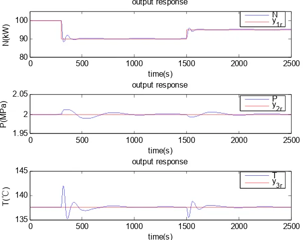
In order to test the tracking performance for the power output under the nominal working conditions, the set-point of power output (load demand) was first decreased from 100 kW to 90 kW at t = 300 s, then increased to 95 kW at t = 1500 s. The responses of output variables and the variations of control variables are shown in Figures 3 and 4 respectively.

Figure 3. Responses of controlled variables.

Figure 4. Responses of manipulated variables.

5.1.2. Tracking the Set-point of Evaporator Pressure

In order to make the test of tracking evaporator pressure at the nominal working condition, the set-point of evaporator pressure was first decreased by 1000 Pa at t = 300 s, then increased by 500 Pa at t = 1500 s. The responses of output variables and the variations of control variables are shown in Figures 5 and 6 respectively.

As shown in Figure 5, the proposed control strategy provides a good tracking performance. The maximum deviation of evaporator pressure is less than 0.001 MPa. It can be seen that the load demand and the superheated temperature deviate from their set-points when the evaporator pressure varies,

0 500 1000 1500 2000 2500

80 90 100

time(s)

N(

kW

)

output response

N y_1r

0 500 1000 1500 2000 2500

1.95 2 2.05

time(s)

P(

M

P

a)

output response

P y_2r

0 500 1000 1500 2000 2500

135 140 145

time(s)

T(

)

℃

output response

T y_3r

0 500 1000 1500 2000 2500

0.7 0.8 0.9

time(s)

μ T

control signal

0 500 1000 1500 2000 2500

2700 2800 2900

time(s)

w

(r/

mi

n)

control signal

0 500 1000 1500 2000 2500

3.5 4 4.5

time(s)

v e

(m/

s)

their maximum deviations are not more than 0.02 kW, 0.1 °C respectively, and the proposed controller drives them back to the set-points quickly.

Figure 5. Responses of controlled variables.

Figure 6. Responses of manipulated variables.

5.1.3. Tracking the Set-point of Evaporator Temperature

In this test, the set-point of the evaporator temperature was decreased by 2 °C at t = 300 s, and then increased by 1 °C at t = 1500 s. The responses of output variables and control variables are illustrated in Figure 7 and 8 respectively.

Figure 7 shows that the evaporator temperature can be controlled to follow the set-points in a timely manner. The maximum deviation of the evaporator temperature is less than 0.5 °C during the test. The load demand and the evaporator pressure deviate from their set-points when the evaporator

0 500 1000 1500 2000 2500

99.95 100 100.05

time(s)

N(

kW

)

output response

N y_1r

0 500 1000 1500 2000 2500

1.998 2 2.002

time(s)

P(M

P

a)

output response

P y_2r

0 500 1000 1500 2000 2500

137.55 137.6 137.65

time(s)

T(

)

℃

output response

T y_3r

0 500 1000 1500 2000 2500

0.88 0.882

time(s)

μ T

control signal

0 500 1000 1500 2000 2500

2849 2850 2851

time(s)

w(

r/

m

in

)

control signal

0 500 1000 1500 2000 2500

4.03 4.035 4.04

time(s)

v e

(m/

s)

temperature varies, but their maximum deviations are less than 1 kW and 0.001 MPa respectively. This clearly demonstrates the good control performance of the proposed LDARC strategy.

Figure 7. Responses of controlled variables.

  Figure 8. Responses of manipulated variables.

5.2. Disturbance Rejection Test

5.2.1. Disturbance in the Throttle Valve Position

Consider the situation that a step disturbance is imposed on the throttle valve position when the waste heat recovery system operates in a steady state. In this simulation, a step decrease of 1% was

0 500 1000 1500 2000 2500

98 100 102

time(s)

N(

kW

)

output response

N y_1r

0 500 1000 1500 2000 2500

1.998 2 2.002

time(s)

P(

M

P

a)

output response

P y_2r

0 500 1000 1500 2000 2500

134 136 138

time(s)

T(

)

℃

output response

T y_3r

0 500 1000 1500 2000 2500

0.86 0.88 0.9

time(s)

μ T

control signal

0 500 1000 1500 2000 2500

2820 2840 2860

time(s)

w

(r/

m

in

)

control signal

0 500 1000 1500 2000 2500

3.8 4 4.2

time(s)

v e

(m

/s

)

introduced to the throttle valve position at t = 300 s and a step increase of 1% made at t = 1,500 s. The responses of the three controlled variables are shown in Figure 9.

Figure 9. Responses of controlled variables.

The variation (disturbance) of the throttle valve position at t = 300 s and 1500 s causes the deviations of the power output, the throttle pressure and the superheated temperature at outlet of the evaporator from their original tracks. The maximum deviations of the three variables are 0.8 kW, 0.02 MPa and 3 °C, respectively. The control action drives these three signals back to their set values after a short period of time, which suggests that the waste heat recovery system is well controlled in the presence of disturbance to the throttle valve position.

5.2.2. Disturbance to the Velocity of Exhaust Gas

In this simulation, a disturbance of the flow rate of exhaust gas is imposed by changing the position of the by-pass valve at the inlet of evaporator when the waste heat recovery system operates in a steady state. A step decrease of 1% at t = 300 s and a step increase of 1% at t = 1500 s were introduced to the velocity of the exhaust gas. The responses of the controlled variables are shown in Figure 10. The disturbance to the velocity of exhaust gas leads to the deviations of the power output, the throttle pressure and the superheated temperature at the outlet of the evaporator, however, under the proposed control scheme, the maximum deviations of these three outputs are only 0.5 kW, 0.01 MPa and 1 °C, respectively. In spite of the disturbance to the exhaust gas, the control action manages to drive the three variables back to their original values within a reasonably short period of time.

0 500 1000 1500 2000 2500

99 100 101

time(s)

N(

kW

)

output response

N y_1r

0 500 1000 1500 2000 2500

1.95 2 2.05

time(s)

P(

M

P

a)

output response

P y_2r

0 500 1000 1500 2000 2500

136 138 140

time(s)

T(

)

℃

output response

Figure 10. Responses of controlled variables.

6. Conclusions

In this paper, the novel LADRC scheme is successfully applied to the design of decentralized controllers for the waste heat recovery system. The ORC process model is achieved by parameter identification technique. Simulation results demonstrate that the proposed control algorithm can provide good tracking performance and well handle disturbances for the waste heat recovery systems.

It should be noted that the design of the control strategy without requiring an accurate mathematical model for the waste heat recovery system is a significant progress for this type of processes. A static coupling method was designed based on the simplified linear ORC model which captured the essential dynamics and interaction of the system. This practical control strategy is easy to understand and implement, making it an appealing method to real applications.

Acknowledgments

This work was supported by the National Basic Research Program of China under Grant (973 Program 2011 CB710706) and the Doctoral Fund of the Ministry of Education of China (20110036110005). These are gratefully acknowledged.

References

1. Hung, T.C.; Shai, T.Y.; Wang, S.K. A review of Organic Rankine Cycles (ORCs) for the recovery of low-grade waste heat. Appl. Energy 1997, 6, 661–667.

2. Tchanche, B.F.; Lambrinos, G.; Frangoudakis, A.; Papadakis, G. Low-grade heat conversion into power using Organic Rankine Cycles—a review of various applications. Renew. Sustain. Energy Rev. 2011, 15, 3963–3979.

3. Wang, E.H.; Zhang, H.G.; Fan, B.Y.; Ouyang, M.G. Study of working fluid selection of organic Rankine cycle (ORC) for engine waste heat recovery. Energy 2011, 36, 3406–3418.

0 500 1000 1500 2000 2500

99.5 100 100.5

time(s)

N(

kW

)

output response

N y_1r

0 500 1000 1500 2000 2500

1.99 2 2.01

time(s)

P(

M

P

a)

output response

P y_2r

0 500 1000 1500 2000 2500

136 138 140

time(s)

T(

)

℃

output response

4. Hung, T.C.; Wang, S.K.; Kuo, C.H.; Pei, B.S.; Tsai, K.F. A study of organic working fluids on system efficiency of an ORC using low-grade energy sources. Energy 2010, 35, 1403–1411. 5. Luján, J.M.; Serrano, J.R.; Dolz, V.; Sánchez, J. Model of the expansion process for R245fa in an

Organic Rankine Cycle (ORC). Appl. Therm. Eng. 2012, 40, 248–257.

6. Wei, D.H.; Lu, X.S.; Lu, Z.; Gu, J.M. Dynamic modeling and simulation of an Organic Rankine Cycle (ORC) system for waste heat recovery. Appl. Therm. Eng 2008, 28, 1216–1224.

7. Quoilin, S.; Aumann, R.; Grill, A.; Schuster, A.; Lemort, V.; Spliethoff, H. Dynamic modeling and optimal control strategy of waste heat recovery Organic Rankine Cycles. Appl. Energy 2011, 88, 2183–2190.

8. Vaja, I.; Gambarotta, A. Dynamic model of an organic Rankine cycle system. Part I—Mathematical description of main components. In Proceedings of 23rd International Conference on Efficiency, Cost, Optimization, Simulation and Environment Impact of Energy, Lausanne, Switzerland, 14–17 June 2010.

9. Vaja, I.; Gambarotta, A. Dynamic Model of an Organic Rankine Cycle System. Part II—The full Model: Description and Validation. In Proceedings of 23rd International Conference on Efficiency, Cost, Optimization, Simulation and Environment Impact of Energy, Lausanne, Switzerland, 14–17 June 2010

10. Wei, D.H.; Lu, X.S.; Lu, Z.; Gu, J.M. Performance analysis and optimization of Organic Rankine Cycle (ORC) for waste heat recovery. Energy Convers. Manag. 2007, 48, 1113–1119.

11. Clemente, S.; Micheli, D.; Reini, M.; Taccan, R. Energy efficiency analysis of Organic Rankine Cycles with scroll expanders for cogenerative applications. Appl. Energy 2012, 97, 792–801. 12. Quoilin, S.; Lemort, V.; Lebrun, J. Experimental study and modeling of an Organic Rankine

Cycle using scroll expender. Appl. Energy 2010, 87, 1260–1268.

13. Lemort, V.; Quoilin, S.; Cuevas, C.; Lebrun, J. Testing and modeling a scroll expander integrated into an Organic Rankine Cycle. Appl. Therm. Eng. 2009, 29, 3094–3102.

14. Desai, N.B.; Bandyopadhyay, S. Process integration of organic Rankine cycle. Energy 2009, 34, 1674–1686.

15. Zhang, J.H.; Zhang, W.F.; Hou, G.L.; Fang, F. Dynamic modeling and multivariable control of Organic Rankine Cycle in waste heat utilizing processes. Comput. Math. Appl. 2012, 64, 908–921. 16. Zhang, J.H.; Li, Y.; Wang, Z.F.; Hou, G.L. Dynamic characteristics and predictive control for

evaporator. In Proceedings of the 2011 International Conference on Advanced Mechatronic Systems, Zhengzhou, China, 11–13 August 2011; pp. 513–518.

17. Hou, G.L.; Sun, R.; Hu, G.Q.; Zhang, J.H. Supervisory predictive control of evaporator in Organic Rankine Cycle (ORC) system for waste heat recovery. In Proceedings of the 2011 International Conference on Advanced Mechatronic Systems, Zhengzhou, China, 11–13 August 2011; pp. 306–311.

18. Han, J. Nonlinear state error feedback control. Control Des. 1995, 10, 221–225.

20. Zheng, Q.; Dong, L.; Gao, Z. Control and Time-Varying Rotation Rate Estimation of Vibrational MEMS Gyroscopes. In Proceedings of IEEE Multi-conference on Systems and Control, Singapore, 1–3 October 2007; pp. 118–123.

21. Huang, H.P.; Wu, L.Q.; Han, J.Q.; Gao, F.; Lin, Y.J. A new synthesis method for unit coordinated control system in thermal power plant-ADRC control scheme. In Proceedings of 2004 International Conference on Power System Technology, Singapore, 21–24 November 2004; pp. 133–138.

22. Dong, L.L.; Zhang, Y.; Gao, Z,Q. A robust decentralized load frequency controller for interconnected power systems. ISA Trans. 2012, 51, 410–419.

23. Gao, Z.Q. Scaling and parameterization based controller tuning. In Proceedings of American Control Conference, Denver, CO, USA, 4–6 June 2003, 4996–4996.

24. Goforth, F.; Zheng, Q.; Gao, Z.Q. A novel practical control approach for rate independent hysteretic systems. ISA Trans. 2012, 51, 477–484.

25. Zheng, Q.; Chen, Z.Z.; Gao, Z.Q. A practical approach to disturbance decoupling control. Control. Eng. Pract. 2009, 17, 1016–1025.

26. Ananth, I.; Chidambaram, M. Closed-loop identification of transfer function model for unstable systems. J. Franklin Inst. 1999, 1055–1061.

27. Haley, T.A.; Mulvaney, S.J. On-line system identification and control design of an extrusion cooking process: Part 1. System identification. Food Control. 2000, 11, 103–120.

28. Xiao, Y.S.; Ding, F.; Zhou, Y.; Li, M.; Dai, J.Y. On consistency of recursive least squares identification algorithms for controlled auto-regression models. Appl. Math. Model. 2008, 32, 2207–2215.

29. Zheng, Q.; Chen, Z.Z.; Gao, Z.Q. A dynamic decoupling control approach and its applications to chemical processes. In Proceedings of American Control Conference, New York, NY, USA, 9–13 July 2007; pp. 5176–5181.