Micromechanical analysis of kinematic hardening in natural clay

Micromechanical analysis of kinematic hardening

in natural clay

Zhen-Yu Yin

a,b,c,d,*

_{, Ching S. Chang}

b

_{, Pierre-Yves Hicher}

c

_{, Minna Karstunen}

d a_{Department of Civil and Environmental Engineering, Helsinki University of Technology, PO Box 2100, 02015 TKK, Finland} b_{Department of Civil and Environmental Engineering, University of Massachusetts, Amherst, MA 01002, USA}

c

Research Institute in Civil and Mechanical Engineering, GeM UMR CNRS 6183, Ecole Centrale de Nantes, BP 92101, 44321 Nantes Cedex 3, France

d_{Department of Civil Engineering, University of Strathclyde, John Anderson Building, 107 Rottenrow, Glasgow G4 0NG, UK}

a b s t r a c t

This paper presents a micromechanical analysis of the macroscopic behaviour of natural clay. A microstructural stress–strain model for clayey material has been developed which considers clay as a col-lection of clusters. The deformation of a representative volume of the material is generated by mobilizing and compressing all the clusters along their contact planes. Numerical simulations of mul-tistage drained triaxial stress paths on Otaniemi clay have been performed and compared the numerical results to the experimen-tal ones in order to validate the modelling approach. Then, the numerical results obtained at the microscopic level were analysed in order to explain the induced anisotropy observed in the clay behaviour at the macroscopic level. The evolution of the state vari-ables at each contact plane during loading can explain the changes in shape and position in the stress space of the yield surface at the macroscopic level, as well as the rotation of the axes of anisotropy of the material.

1. Introduction

In order to take into account the anisotropic mechanical behaviour of clay, a number of elastic–plastic stress–strain models have been developed, such as the models byNova (1985), Dafalias (1986), Whittle and Kavvadas (1994), Pestana and Whittle (1999), Wheeler et al. (2003), Dafalias et al. (2006), etc. Hashiguchi and Mase (2007)developed a model employing a rotational kinematic hardening function for modelling the anisotropy of cemented sand.Yang et al. (2006)proposed a middle surface model using three pseudo-yield surfaces. A kinematic hardening rule was applied to the second pseudo-yield surface for modelling the anisotropic behaviour of sand. More recently, various kinematic hardening rules have been, respectively, investigated for frozen soils, unsaturated soils, and granular media byLai et al. (2008), Muraleetharan et al.(2008), and Tsutsumi and Kaneko (2008). The key feature of these models is to adopt an asymmetrical yield surface for the modelling of inherent anisotropy due to the geological formation process, and to incorporate a kinematic hardening law for the modelling of induced anisotropy, in which the kinematic hardening law describes how the yield surface moves and changes its shape with the applied stresses. Both the initial yield surface and the kinematic hardening law of these models have been constructed phenomenologically from experimental results. Due to the complex nature of soil behaviour, it is difficult to construct a kinematic hardening law that is simple, effective, and at the same time, capable of capturing correctly the salient features of soil behaviour.

Besides the kinematic hardening approach, a potentially attractive way of modelling anisotropic material is the microstructural approach, in which the stress–strain relationship of a representative ele-ment is obtained by mobilizing contact planes of various orientations. The concept goes back to Taylor and Budiansky in their models for polycrystalline material (e.g.,Batdorf and Budianski, 1949). Similar approaches can also be found in the models of rock and soils (e.g.,Calladine, 1971; multilaminate models byPande and Sharma, 1982; Cudny and Vermeer, 2004), in the models of concrete (e.g., micro-plane model byBazant et al., 1995), and in the models of granular materials and sands (e.g.,Chang and Liao, 1990; Chang and Gao, 1995; Chang and Hicher, 2005; Nicot and Darve, 2007).

The proposed approach can better model anisotropic material due to the following two reasons: (1) the state variables (local stress and strain) are naturally different in the contact planes according to their orientations related to the applied load. Since contact stiffness and contact strength are stress-dependent, this would lead to different properties for each plane. Thus, the applied stress would create anisotropy for the material in a natural manner; (2) the evolution of the state variables (local stress and strain) is attained directly from the applied stress on each contact plane. There is no need to define a yield surface and a kinematic hardening rule in order to follow the evolution of the anisotropy.

In this paper, the development of a microstructure based elasto-plastic constitutive model is first presented. The model is then used to predict multistage drained triaxial stress path tests on Otaniemi clay. A numerical microstructural investigation is also carried out, which is intended to explain the induced anisotropy through the behaviour on contact planes. Finally, the microstructural model is used to construct the yield surface and to explain macro kinematic hardening of yield surface, i.e., how the yield surface expands, rotates, and changes its shape due to different stress paths.

2. Constitutive model

A clay particle is usually platy in shape. The size for a platy particle generally ranges from 0.01 to 1

lm depending on the clay type (e.g., montmorillonite, illite or kaolinite). Clay particles attract each

other due to surface forces among particles such as chemical, electrostatic, van der Waals forces, etc. These forces pull together the particles to form particle-clusters. The size of the clusters continues to grow until the clusters are large enough so that the cluster weight, due to gravitation, becomes signif-icantly larger than the inter-particle surface forces. At this stage, the cluster looses its potential to attract further clay particles, and the size of clusters stops to grow. The ultimate cluster size depends on the clay particle type, the liquid inside the pores, and its sedimentation history.

From the photos of clay material under scanning electron microscopes, clusters formed by platy clay particles can be identified as rotund shape, although the microfabric within a cluster may be either a flocculate or dispersed type structure (Hicher et al., 2000).

considered as a collection of clusters, can be modelled by analogy to granular material. This explains why sand and clay have similar qualitative behaviour even though each material consists of different constituents (Biarez and Hicher, 1994).

The present model is extended from the sand model developed byChang and Hicher (2005). In this model, clay is envisioned as an aggregate of clusters. The deformation of a representative volume of the material is generated by mobilizing and compressing all clusters. Thus, the stress–strain relationship can be derived as an average of the deformation behaviour of local contact planes in all orientations. For contact planes in the

a

th orientation, the local forcesfa

j and the local movementsd a

i can be denoted as follows:fa

j ¼ ffna;fsa;ftaganddai ¼ fdan;das;dtag, where the subscriptsn,s, andtrepresent the components in the three directions of the local coordinate system as shown inFig. 1. The direction outward normal to the plane is denoted asn; the other two orthogonal directions,sandt, are tangential to the plane.

2.1. Density state of clay

One of the important elements to consider in modelling clay behaviour is the critical state concept. At critical state, the clay material remains at constant volume while it is subjected to a continuous dis-tortion. The void ratio corresponding to this state is termed critical voidec, which is a function of the effective mean stressp= (

r

x+

r

y+

r

z)/3 (all stress terms used in the part of constitutive model refer to effective stress). The relationship has traditionally been written as follows:

ec¼ec0kln p pcr0

ð1Þ

The two parameters (ec0,pcr0) represent a reference point on the critical state line. For convenience, the

value ofpcr0is taken to be 1 kPa. The critical state line can be defined by two parameters ec0and k.

Using the critical state concept, the density state of an assembly under a given mean effective stress is defined as the ratioe/ec, whereeis the void ratio of the assembly andecthe critical void ratio at the same given stress state.

The relationship between void ratio and isotropic stress in semi-log scale (e–logp) is assumed to be linear. However, some investigators prefer to use a linear relationship between log

e

v–log pfor clay with large deformation (Hashiguchi, 2008).

2.2. Inter-cluster behaviour

Since contact forces and applied stresses have different units, it is troublesome to compare their magnitudes. Thus, local stresses and local strains are introduced for convenience. We define a local stress

s

a

[image:3.595.168.435.576.758.2]

i and a local strain

c

ai, which are directly related to the local forcefjaand the local movement da_i at each contact, given by

s

a

i ¼

Nla

3V f a

i ;

c

ai ¼d

a

i=l

a

ð2Þ

wherela is the length of the branch vector, which joins the centroids of two contacting clusters.Vis the volume of the representative element. Nis the total number of contacts. The form of the local stress is derived from the static hypothesis given byLiao et al. (1997)

_

faj ¼

r

_ijAikl

a

k ð3Þ

whereAikis the inverse of fabric tensorAik¼ 1 V

PN

a¼1l

a il

a k

h i1

For the case of an isotropic fabric, it can be derived that Aik= 3V/(Nl2)dik, where dik is the Kronecker delta. In this case, Eq. (3) implies

r

jinaj ¼Nl a

=ð3VÞfa

i . Therefore, the local stress defined in Eq.(2)is equal in magnitude to the traction resolved from the applied stress on the contact plane (i.e.,

s

a

i ¼

r

jinaj) for an isotropic packing struc-ture. It is to be noted that the local stress

s

a

i is not the true stress on the physical contact area between the two clusters. It should be rather viewed as a normalized form of the contact force.

In the local coordinate system, the local stress and local strain are, respectively, denoted as

f

s

a

n

s

as

s

atgandf

c

an

c

as

c

at g. For convenience, we use the notation

r

a¼

s

anfor local normal stress and the notation

e

a_¼

_c

a

n for local normal strain in the following sections.

2.2.1. Elastic part

The inter-cluster behaviour can be characterized as the relationship between local stress and local strain, given by

s

a

i ¼kaij

c

aj ð4Þ

in which the stiffness tensor can be related to the contact normal stiffness,ka

n, and shear stiffness,kar,

ka

ij ¼kannianaj þkarðsaisaj þtaitajÞ ð5Þ

The inter-cluster stiffness can be expressed as the form adopted for sand grains by Chang et al. (1989), given by

ka_n ¼ka_n0

r

a

pref

!n

; ka_r ¼krRkan¼krRkan0

r

a pref

!n

ð6Þ

where

r

ais the local stress in normal direction,prefis the standard reference pressure taken as 1 kPa, andkrRis the ratio of shear to normal stiffness.kan0;krRandnare material constants. The value ofnis

found to be 0.33 for two elastic spheres according to Hertz–Mindlin’s formulation (1969). Based on experimental measurements of elastic modulus under different confining stress, the value ofn has been found to be 0.5–1.0 for clay.

2.2.2. Plastic part

2.2.2.1. Shear sliding. Plastic sliding often occurs along the tangential direction of the contact plane with an upward or downward movement (i.e., dilation or contraction). The dilatancy equation used here is modified from the equation adopted for sand byChang and Hicher (2005), given by

d

e

p

d

c

p¼b

s

r

tan/l

s

r

a

1 e

ec

ð7Þ

The modified equation allows more flexibility in modelling the performance of different material behav-iour. In this equation,a,b, and/_lare inter-cluster property constants;ecis the critical void ratio for the clay. When the void ratioeis equal to the critical void ratio, zero dilation holds. It is noted that the state variablese andecof the clay are at a macro-scale of the cluster assembly, which is used to regulate the dilation of indi-vidual inter-cluster contacts. It is reasonable to consider the micro variable as a function of the macro-state, because the inter-cluster behaviour is indeed influenced by the density state of the specimen.

Note that the shear stress

s

and the rate of plastic shear straind

c

p_{in Eq.(7)are defined as}

s

¼

ffiffiffiffiffiffiffiffiffiffiffiffiffiffiffiffi

s

2

s þ

s

2t

q

and d

c

p ¼

ffiffiffiffiffiffiffiffiffiffiffiffiffiffiffiffiffiffiffiffiffiffiffiffiffiffiffiffiffiffiffiffi

ðd

c

psÞ2þ ðd

c

ptÞ

2 q

ð8Þ

The yield function is assumed to be of Mohr–Coulomb type, given by

F1ð

s

;

r

;

j

1Þ ¼

s

rj

1ð

c

pÞ ¼0 ð9Þ

where

j

1(

c

p) is an isotropic hardening/softening parameter. The hardening parameter is defined by a

hyperbolic function in the

j

1–

c

pplane, which involves two material constants:/p andkp.

j

1¼

kptan/p

c

p

r

tan/_pþkp

c

p

ð10Þ

When plastic deformation increases,

j

1 approaches asymptotically tan/p. For a given value of

r

, the initial slope of the hyperbolic curve is kp=

r

. Under a loading condition, the shear plastic flow in the direction tangential to the contact plane is determined by a normality rule applied to the yield function. However, the plastic flow in the direction normal to the contact plane is governed by the stress-dilatancy equation in Eq.(7). Therefore, the flow rule is non-associated.

The value ofkp is found to be linearly proportional toknso that

ka_p¼kpRkna¼kpRkan0

r

a pref

!n

ð11Þ

The ratiokpRis a material parameter.

The internal friction angle/_lis a constant for a given material. However, the peak friction angle,/_p, on a contact plane is dependent on the density state of neighbouring clusters, which can be related to the void ratioeby

tan/_p¼ ec

e

m

tan/_l ð12Þ

wheremis a material constant (Biarez and Hicher, 1994).

In a loose structure, clusters can rotate more freely, preventing the inter-cluster shear force from fully mobilizing the sliding resistance. The peak frictional angle/p is smaller than /l. On the other hand, a dense structure provides a higher degree of interlocking, which requires more effort to mobi-lize the clusters in contact. In this case, the peak frictional angle/pis greater than/l. When the dense structure starts to dilate, the degree of interlocking relaxes. As a consequence, the peak frictional angle is reduced, which results in a strain-softening phenomenon.

2.2.2.2. Normal compression. In order to describe the compressible behaviour between two clay

clus-ters, a second yield function is hence added. The second yield function is assumed to be as follows:

F2ð

r

;

j

2Þ ¼

r

j

2ð

e

pÞ for

r

>

r

p ð13Þ

where the local normal stress

r

and local normal strain ep are defined in Eq. (3). In analogy to the macro volume compression behaviour, we express the hardening function

j

2(ep) in a semi-logarithmic

form given by

j

2¼

r

p10e

p_=c

p _or

_e

p_¼c

plog

j

2

r

p

ð14Þ

wherecpis the compression index for the compression curve plotted in theep–logrplane. When the compression

r

is less than

r

p, the plastic strain produced by the second yield function is null. Thus,

r

p in Eq.(12)corresponds to the pre-consolidation stress in soil mechanics.

2.2.3. Elasto-plastic relationship

_

s

a

i ¼k

ap

ij

c

_

a

j ð15Þ

Since detailed derivation of the elasto-plastic stiffness tensor is standard, it will not be given here.

2.3. Stress–strain relationship

2.3.1. Macro–micro relationship

The stress–strain relationship for an assembly of clay clusters can be determined from integrating the inter-cluster behaviour at all contacts. During the integration process, a relationship is required to link the macro and micro variables.

In a micromechanical expression, following the Love–Weber formula, the stress increment

r

_ijcan be obtained by adding the diatic product of the contact force and the branch vectors for all contacts (Christofferson et al., 1981; Rothenburg and Selvadurai, 1981). In terms of local stress, it is

_

r

ij¼ 1

V X

N

a¼1

fjal

a

i ¼ 3

N X

N

a¼1

s

a

jnai ð16Þ

In terms of the local stress on the

a

th contact plane defined in Eq.(2), the static hypothesis of Eq.(3) becomes

_

s

a

j ¼

r

_ijBaiknak ð17Þ

where the tensorBa_ikin Eq.(17)is defined asBa_ik¼N=ð3VÞAikðlaÞ2:

Using the principle of energy balance, which states that the work done in a representative volume element is equal to the work done on all inter-cluster planes within the element,

r

iju_j;i¼ 1

V XN

a¼1

fjad_aj ¼ 3

N XN

a¼1

s

a

j

c

_aj; ð18Þ

Substituting the local stress in Eq.(17)into Eq.(18), the relationship between the strain of assem-bly and inter-cluster strain is obtained

_

uj;i¼ 3

N XN

a¼1

_

c

a

jn

a

kB

a

ik ð19Þ

where

c

_jis the local strain between two contact clusters,nkthe unit vector of the branch joining the cen-tres of two contact clusters, andNthe total number of contacts, over which the summation is carried out. Using Eqs. (15), (19), and (17), the following relationship between stress and strain can be obtained:

_

ui;j¼Cijmp

r

_mp ð20Þ

where

Cijmp¼ 3

N X

N

a¼1

ðkep_jpÞ1naknanB

a

ikB

a

mn ð21Þ

The summation in Eq.(21)can be expressed by a closed-form solution for some limited conditions such as the elastic modulus of randomly packed equal-size particles (Chang and Gao, 1995). However, in an elastic–plastic behaviour, due to the nonlinear nature of the local constitutive equation, a numer-ical calculation with an iterative process is necessary to carry out the summation in Eq. (21) (see Chang and Hicher, 2005).

2.4. Summary of parameters

The material parameters are summarised as follows:

(1) Microstructural descriptions (two parameters)

(2) Inter-cluster properties (nine parameters) - Inter-cluster elastic constants:kn0;krR, andn; - Inter-cluster friction angle:/l andm;

- Inter-cluster plastic compression index and plastic shear stiffness ratio:cpandkpR; - Dilation constants:aandb

(3) Density state of the assembly (three parameters) - Critical state for the soil:kandec0

- Reference void ratio,e0, on the isotropic compression line atp= 0.001 MPa.

The size of a clay clusterdcan be estimated from an electron microscopic scanning photograph. The value of N/Vis not easy to obtain directly from the clay experiments. According to the experimental data byOda (1977)for three mixtures of spheres, the contact number per unit volume can be approx-imately related to the void ratio by

N V ¼

12

p

d3ð1þeÞe ð22Þ

Here we use this equation as a first-order approximation to estimateN/Vfor clay by treatingdas the mean size of the clay clusters. It is noted that the value of contact number per unit volume changes with void ratio. The evolution is accounted for during the deformation process.

The mean sizedof the clay clusters is assumed to be 4

lm according to the observations from

Scan-ning Electronic Microscope (SEM) results on kaolinite (Hicher et al., 2000). The exponentnis generally between 0.7 and 1.0 for clay, and a typical value of exponentmis 1. From an isotropic compression test, four parameters can be determined; namely,e0,k,kan0, andcp. The void ratioe0andkcan be

mea-sured directly from the compression line. The values ofka

n0andcpcan be calibrated from the slopes of

the compression and rebound curves. The other parameters/_l,kpR,krR, a,b, andec0can be obtained

from drained triaxial tests (as shown later).

3. Test simulation and analysis

3.1. Review of experimental results

The anisotropic behaviour of a natural clay, Otaniemi clay in southern Finland, is presented herein with reference to experimental results based on the work ofWheeler et al. (2003) and Karstunen and Koskinen (2004). Otaniemi clay is classified as a high-plasticity clay with the following mineralogical compositions: quartz 23%, feldspar 46%, illite 15%, chlorite 10%, and kaolinite 5%, determined at ETH Zurich byMesserklinger et al. (2003). The tests on Otaniemi clay were all performed on samples taken at depths of 3.4–4.7 m. Some physical properties of Otaniemi clay at this depth are presented inTable 1.Wheeler et al. (2003)indicated that there is a noticeable natural variation within this 1.2 m thick clay layer.

To investigate the induced anisotropic behaviour and the resulting kinematic hardening of the yield surface, 26 drained triaxial tests with different effective stress paths were selected (20 of them can be found inWheeler et al., 2003). All tests were conducted using conventional triaxial cells with devia-toric force applied by dead weight loading for both compression and extension. Stress increments were generally applied at daily intervals with the increment size depending on the requirements of the individual test stage. Each test consists of two loading stages (seeFig. 2):

(1) At the first loading stage, the specimen is loaded in a drained condition at a constant value of

g

1

to a final stress state (p0

1;q1), and then unloaded with

g

1unchanged (where

g

=q/p0,q=

r

1

r

3,

andp0_{¼ ð}

_r

0

1þ2

r

03Þ=3 for triaxial condition, with positive and negative

g

representing

(2) At the second loading stage, the specimen is again loaded in a drained condition at a different constant value of

g

2to another final stress state (p02;q2). All tests were classified in three series

of tests (seeTable 2, Wheeler et al., 2003):

Series A:The samples were first loaded at various values of

g

1 (ranging from 0.65 to 1.08) to a

given stress state, and then each sample was loaded at a suitable alternative value of

g

2 varying

from 0.09 to 0.74.

Series B: The samples were first loaded at

g

1= 0.75 to p01¼40 kPa, and then each sample was

loaded at a different value of

g

2varying from0.52 to 0.51. The clay is subjected in situ to a value

of

g

about 0.75.

Series C: The samples were first loaded at

g

1= 0.11 to p01¼45 kPa, and then at the second stage,

each of the samples was loaded at values of

g

2 varying from0.58 to 0.83.

For Series B and C, the specimens were consolidated up to 40–45 kPa at the end of the first loading stage. The stress is higher than the in situ overburden pressure, which helps to reduce the sample’s non-homogeneities due to the sampling process.

3.2. Calibration of model parameters

To calibrate the model parameters, we selected two experimental tests: (1) isotropic consolidation test (CID2241 listed inTable 2), and (2) an anisotropic consolidation test followed by an undrained triaxial compression (CAUC2239). The calibrated list of parameters is given inTable 3a. The parame-ters are calibrated based on the following process.

Parameter k= 0.46 was determined from the slope of the experimental consolidation curve (see Fig. 3a). The inter-cluster friction angle /l is determined from the slope of the critical state line in p0_{–qplane. A value of/}

l= 30°was determined from an undrained triaxial test (seeFig. 3b). A typical value ofm= 1 is used. The value ofpcr0andec0can be determined from the state (stress and void ratio)

p'

q

loading with

1

unloading with

1

reloading with

2

Series A:

1

= [-0.65, 1.08]

2

= [0.09, 0.74]

Series B:

1

= 0.75

2

= [-0.52, 0.51]

Series C:

1

= 0.11

[image:8.595.57.537.104.422.2]

2

= [-0.58, 0.83]

[image:8.595.59.533.105.225.2]

Fig. 2. Schematic description for test Series A, B, and C.

Table 1

Physical properties of Otaniemi clay of depth 3.4–4.7 m (afterWheeler et al., 2003).

Index property Value

Water content,w(%) 85–130

Liquid limit,wl(%) 80–111

Plastic limit,wp(%) 26–29

Plasticity index,Ip 54–82

Percentage of particles <0.002 mm, C1% 65–83

Organic content, Hm (%) 0–0.7

Specific gravity, Gs 2.76–2.80

Undrained shear strength, cu (kPa) 6–9

Sensitivity, St 7–14

[image:8.595.174.426.222.407.2]

corresponding to the critical state. The values of pref and e0 can be determined by an isotropic line,

whereprefis 1 kPa with the point (pref,e0) appearing on the isotropic line (see Fig. 3a).Fig. 3c shows

a slight influence of krRand kpRon simulating the isotropic consolidation test which means krRand kpR are not sensitive for IC test. Other parameters can be obtained by curve fitting, as shown in Fig. 3d–i, as follows:

(1) Inter-cluster elastic constants:kn0;krRandn;

The exponent n= 1 was considered which provides a linear

j

-line (unloading–reloading curve ine–logp0_{of the consolidation test). The value ofk}

n0was determined from the

j

-line, as shown

inFig. 3d.krRwas determined from the

e

v–

e

1(volumetric strain versus axial strain) curve of the iso-tropic consolidation test (seeFig. 3e).

[image:9.595.64.540.105.428.2]

(1) Inter-cluster normal hardening rule:cp and

r

0p0; Table 2

Drained triaxial tests on Otaniemi clay.

Test number Depth (m) w(%) ei First loading Second loading

g1 p01ðkPaÞ q1ðkPaÞ g2 p02ðkPaÞ q2(kPa) Series A CAD2260 4.03–4.14 97.8 2.73 1.08 33 32.4 0.1 150 15.3

CAD2463 3.47–3.59 119 3.43 1 37 37 0.3 100 30.3

CAD2464 3.64–3.76 114.9 3.26 0.89 38 33.8 0.33 101 33.8 CAD2261 4.03–4.14 92.5 2.62 0.79 37 29.2 0.1 150 15.4 CAD2530 4.03–4.14 101.4 3.1 0.6 40 20.32 0.32 71 22.5 CAD2251 4.20–4.31 90 2.51 0.6 40 24.1 0.09 150 14.1 CAD2280 4.37–4.48 93.6 2.54 0.51 50 25.4 0.1 120 12.5 CAE2586 3.62–3.73 112.4 3.23 0.43 44 18.8 0.51 96 49.2 CAD2276 4.56–4.68 79.4 2.59 0.26 48 12.4 0.11 150 15.9 CAD2514 4.23–4.34 85.4 2.98 0.21 36 7.5 0.74 60 44.5 CAE2496 4.20–4.31 93.5 2.54 0.34 31 10.5 0.1 66 6.7 CAE2544 4.37–4.48 88.1 2.98 0.6 33 19.8 0.51 66 33.7 CAE2513 4.03–4.14 104.7 2.91 0.65 29 18.8 0.61 60 36.8

CID2241 4.02–4.14 105 2.81 0 151 0 0.11 201 22.5

CID2515 4.40–4.51 92 2.2 0 60 0 0.6 100 60

CID2291 4.37–4.48 100.4 2.86 0 37 0 0.1 116 12

CID2403 3.62–3.73 114 3.3 0 42 0 0.42 99 42

Series B CAD2443 4.23–4.34 89.1 2.56 0.75 40 30 0.51 100 51

CAD2425 4.06–4.17 101.5 3.01 0.22 97 21

CAE2529 4.37–4.48 84.1 2.50 0.26 78 20

CAE2522 4.12–4.23 101.1 2.74 0.52 60 31

Series C CAD2424 4.03–4.14 108.5 3.10 0.83 60 50

CAD2423 4.20–4.31 94.4 2.61 0.58 99 57

CAD2422 4.05–4.17 102.8 2.93 0.11 45 5 0.11 100 36

CAE2561 3.95–4.06 101.1 2.93 0.45 87 39

[image:9.595.64.540.481.577.2]

CAE2550 4.32–4.43 90.8 2.63 0.58 84 49

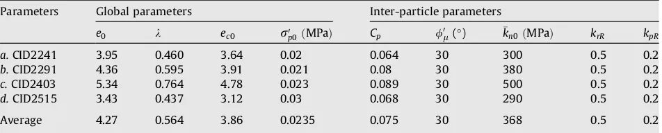
Table 3

Values of model parameters for Otaniemi clay.

Parameters Global parameters Inter-particle parameters

e0 k ec0 r0p0ðMPaÞ Cp /0l(°) kn0ðMPaÞ krR kpR

a.CID2241 3.95 0.460 3.64 0.02 0.064 30 300 0.5 0.2

b.CID2291 4.36 0.595 3.91 0.021 0.08 30 380 0.5 0.2

c.CID2403 5.34 0.764 4.78 0.023 0.089 30 500 0.5 0.2

d.CID2515 3.43 0.437 3.12 0.03 0.068 30 290 0.5 0.2

The value of cpwas determined by keeping the isotropic consolidation line parallel to the critical state line (seeFig. 3f). The initial value of the pre-consolidation pressure

r

0

p0due to the clay deposition

history was determined, as shown inFig. 3f.

(1) Inter-cluster shear hardening rule:kpR;

The value of kpRwas determined from the q–

e

1curve of an undrained compression test at small strain, as shown inFig. 3g.

(1) Dilation constantsa andb were determined from an undrained compression test (seeFig. 3h and i); from this curve, combined values ofaandbcan be chosen by curve fitting. Parameters a andb governing the amount of volumetric dilation have a significant influence on the peak strength of the q–

e

1 curve. Fig. 3h shows that different effective stress paths, with a similar shape of the yield curve, can be described by different values ofaandb.

1 2 3 4

1 10 100

p' (kPa)

e

CID2241

1 = 0.46

e0 = 3.95

0 10 20 30 40

0 10 20 30

p' (kPa) q ( kP a) CAUC2239 Consolidation Shearing 1

M = 1.2

pcrit = 16 kPa

1.5 2 2.5 3 3.5 4

0.1 1 10 100

p' (kPa)

e

CID2241 Simulation

Simulation use

krR = 0.1, kpR = 0.4;

krR = 0.1, kpR = 0.6;

krR = 0.5, kpR = 0.4

Clay deposition K_{( = 0.75)}0 = 0.5

K0 = 1.0

( = 0)

1.5 2 2.5 3 3.5 4

0.1 1 10 100

p' (kPa)

e

CID2241 Simulation

kn0 = 200

kn0 = 400

kn0 = 300

Clay deposition

K0 = 0.5

( = 0.75)

K0 = 1.0

( = 0)

0

10

20

30

40

-5 -2.5 0 2.5 5

1(%) v (% ) CID 2241 Simulation

krR = 0.1

krR = 0.3

krR = 0.5

under kpR = 0.4

1.5 2 2.5 3 3.5 4

0.1 1 10 100

p' (kPa)

e

CID2241 Simulation

'p0 = 16 kPa

Clay deposition

'p0 = 24 kPa

'p0 = 20 kPa

K0 = 0.5

( = 0.75)

K0 = 1.0

( = 0)

Critical state line

0 5 10 15 20

0 0.05 0.1 0.15

1 (%)

q ( k Pa ) CAUC2239 Simulation

kpR = 0.4

kpR = 0.2

kpR = 0.1

0 10 20 30 40

0 10 20 30 40

p' (kPa) q ( kP a) CAUC2239 Simulation

a = 5, b = 20 a = 3, b = 5

a = 3, b = 20

0 10 20 30 40

0 2 4 6

1 (%)

q (

kPa

)

CAUC2239 Simulation

a = 5, b = 20

a = 3, b = 5

a = 3, b = 20

a

b

c

d

e

f

[image:10.595.64.528.81.541.2]

g

h

i

Due to the large variation in the characteristics of the samples, three additional isotropic consoli-dation tests were selected to determine the model parameters by using the same procedure of calibra-tion. All determined parameters and the averaged parameters are summarised inTable 3. The average parameters were used to simulate isotropic consolidation test and compared with all data from the four experimental results inFig. 4b. The average parameters were also used to simulate the undrained triaxial compression tests and compared with experimental results as shown inFig. 4c. The same set of parameters is also used to simulate drained triaxial compression tests for both normal and over con-solidated Otaniemi clay as shown inFig. 4d and e. Unfortunately, the experimental results on drained triaxial compression tests from Otaniemi clay at this field site are not available for comparison with the model simulation. However, the simulation appears to capture the main features of the drained triaxial compression behaviour for general clay. Thereby, the average values of the parameters seem to be suitable for representing the average properties of tested samples from Otaniemi clay.

3.3. Test simulation and microstructural analysis

In this section, three different cases of consolidation tests, namely

g

1=

g

0,

g

2<

g

1, and

g

2>

g

1

were analysed by means of the micromechanical approach, where

g

0,

g

1, and

g

2 correspond to,

respectively, the clay deposition, the first, and the second stages of loading. These tests are selected from Table 2.

The simulation of each test begins with a consolidation loading with

g

0= 0.75, which corresponds

to the K0 condition in the field. Along this stress path, the specimen is loaded to p0= 15.7 kPa and q= 11.75 kPa, which is equivalent to an effective overburden stress 23.5 kPa at 4 m depth below ground. This process is used to simulate clay deposition in the field, as shown in the upper part of Fig. 5a, marked by pointsa,b, c. The corresponding points on ae–logp0 _{curve are shown inFig. 5b.}

1 2 3 4

1 10 100

p' (kPa)

e

CID2241

CID2291

CID2403 CID2515

Simulation

0

5

10

15

20

25

1 10 100

0 10 20 30 40

0 10 20 30 4

p' (kPa)

q (

kP

a)

0 CAUC2239

Simulation

p' (kPa) v (%

)

CID2241 CID2291 CID2403

CID2515 Simulation

0 0.5 1 1.5

0 5 10 15 20 25

1 (%)

q/

p'

OCR = 5

OCR = 1

Confining pressure 'IC = 100 kPa

-5

0

5

10

15

20

0 5 10 15 20 25

1 (%) v (%

)

OCR = 5

OCR = 1

a

d

e

[image:11.595.69.538.79.407.2]

b

c

Then, the specimen is unloaded to a very small stress value, along the path of

g

= 0.75. This is a sim-ulation of the sampling process, in which the sample is extracted from 4 m depth to the ground sur-face, as the rebound curve shown inFig. 5a and b, marked byc,d. Point1corresponds to the state of the specimen to be used in the laboratory for the first stage loading test.

The first stage loading is then simulated. The specimen is loaded with a constant

g

1to a pressure

greater than the point ofp0_{= 15.7 kPa andq= 11.75 kPa, as shown inFig. 5a and b, marked by 1, 2, 3,} and 4. The specimen is again unloaded to a very small value, along the path of

g

1. The rebound curve is

marked by points 4 and 40_.

Subsequently, the second stage loading is performed. The specimen is loaded with a constant

g

2to

a pressure greater than that of point 4 (i.e., the ending point of the first loading stage), as shown inFig. 5a and b, marked by points 5, 6, 7, 8, and 9. At this point, the simulation is completed.

For each test, the simulation results ofe–logp0_{curves are compared with the experimental data to} evaluate the suitability of the model. The apparent yield points obtained from the experiments are also compared with those obtained from the predicted curves.

In addition, the local stress–strain behaviour at contact planes of various orientations is also plotted for analyses. The detailed plots for contact planes of various orientations will be described in a later section.

3.3.1. Case 1:

g

1=

g

0

Four consolidation tests (Series B inTable 2) along theK0-consolidated stress path (

g

1=

g

0= 0.75)

were simulated. After the clay deposit simulation along

g

0= 0.75, the first and second loading stages

were then simulated. In this case we focus only on the results of the first loading stage, which are plot-ted inFig. 6and compared with experimental results. Good agreement between the experimental data and the simulation was achieved for the ev–logp0 curves. The apparent yield point can be obtained from a linear plot of ev–p0 curve using a bilinear construction method as suggested by Mitchell (1970) and Karstunen and Koskinen (2008). Theev–p0plot is shown inFig. 6b for both model simula-tion and experimental results. The yield points determined from both model simulasimula-tion and experi-mental results are very close for this case.

The model simulation for the behaviour on the contact planes are also plotted to show the relations between the representative element and the different contact planes. Since the loading is symmetric around thez-axis, the orientation of a given contact plane can be defined by an inclined anglehwhich is between the branch vector and thez-axis of the local coordinate system, as shown inFig. 5a. The angleshselected are 0°, 18°, 28°, 45°, 55°, 72°, and 90°(h= 0°corresponds to a horizontal plane), as shown in thex–zplane (Fig. 5c).

Fig. 7shows the local stress–strain relationships for the contact planes in the selected orientations. The local stress paths are plotted in the

s

–

r

plane, as shown inFig. 7a, for both the clay deposition

logp' e

b a

c

d

1 _{2 3}

4

5 ₆

7 8

9 a-b-c: simulation for the history of clay deposition in field with 0

c-d: sampling taken from ground (unloading)

1-2-3-4: first loading stage with 1

4-4': unloading 5-6-7-8-9: second loading stage with 2

4'

Z X

0o

90o 18o

28o 45o

55o

72o at 4 m depth 'p0

p' q

a b

c

d

1 2 3

4

4'

5 6

7 8

9 1

2 K0

'p

[image:12.595.63.533.82.270.2]

a

b

c

Fig. 5. (a and b) Simulation procedure and selected steps for rose diagram, and (c) five inter-particle orientations located on the

stage and the first loading stage. The local stress paths are different from one contact plane to another, under the load applied to the specimen. The shear component becomes more significant when the plane is more inclined. The maximum slope is near the planes oriented at 55°. No shear component is generated for the horizontal and vertical plane contacts (0° and 90°). For the selected planes, the slope of the local stress path increases from plane orientation 0°to 55°and decreases from 55°to 90°. In the local normal stress–strain curves (seeFig. 7b), contact planes of all orientations yield simul-taneously when the loadpapplied to the specimen reaches its yield point (i.e., 15.7 kPa as shown in Fig. 6a and b). The elastic limits decrease from plane orientation 0° to 90°. These elastic limits were created due to the previous load applied to the specimen during the clay deposition. In the local shear strain versus normal strain curves (seeFig. 7c), the amount of shear strain agrees with the slope of the local stress path, i.e., the larger slope leads to a larger shear strain.

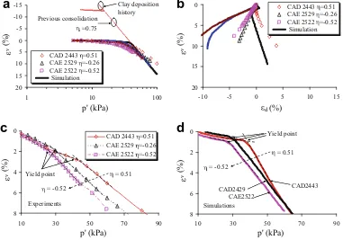
InFig. 8, the distribution of local stresses and strains versus plane orientations (in rose diagram) are plotted for the ending step c for the clay deposit stage and the selected steps 1, 2, 3, and 4 for the first loading stage (seeFig. 5a and b).

It is noted that the normal stress

r

and shear stress

s

distributions due to the clay deposition show a difference in all orientations, thus creating induced anisotropy of this material. This may lead to an irrecoverable microstructure alteration, thus producing and the inherent anisotropy.

The distributions expand in size from step 1 to 4 while keeping the same shape (seeFig. 8a and b). Originally, the distribution of normal stress

r

is a point representing zero stresses in all directions. At the end of the clay deposition (step c inFig. 5a and b), the distribution expands to the location of the bold line plotted in Fig. 8a. This location represents the pre-consolidation pressures of all contact planes. During the sampling (c, d inFig. 5a and b), the distribution shrinks to the point of origin as an unloading process. Then, it expands again during the first loading stage. At step 3, the distribution reaches the bold line. It is noted that, during steps 1, 2, and 3, all contact planes are elastic until the

-5

0

5

10

15

20

1 10 100

0

2

4

6

8

10

0 5 10 15 20 25 30

p' (kPa)

v (%) _{CAD 2443}

CAD 2425 CAE 2529 CAE 2522 Simulation Yield point for experiments

Yield point by model Clay deposition

0 =0.75

p' (kPa)

v (%

) CAD 2443 CAD 2425 CAE 2529 CAE 2522 Simulation

First loading stage 1

[image:13.595.120.479.82.207.2]

a

b

Fig. 6. Model prediction for tests with stress ratiogthe same as that of previous consolidation stageg0.

-0.01 0 0.01 0.02 0.03

0 0.02 0.04 0.06

(Mpa)

(MP

a)

18o 28o 45o

72o 55o

0o 90o

0 = 0.75 1 = 0.75

-0.02

0

0.02

0.04

0.06

0 0.02 0.04 0.06

(Mpa)

18o 28o 45o 72o55o

0o 90o

0 = 0.75 1 = 0.75

0o 90o

-0.02

0

0.02

0.04

0.06

-0.005 0 0.005 0.01 0.015 18o 28o72o45o

55o

0o 90o

[image:13.595.72.527.258.421.2]

a

b

c

distribution reaches the bold line. Then, all contact planes reach their pre-consolidation pressures simultaneously, and all planes begin to behave plastically, which can also be seen inFig. 7b. At this point, the sample behaviour displays a sharp change in direction in theev–logp0as shown inFig. 6a, representing the apparent yield point of the soil sample.

Fig. 8c shows the stress ratio at contact in all orientations. The elastic limits have not been exceeded in the first loading stage. Hence, small shear strains are expected.

Fig. 8d shows the distribution of normal strain, which implies slight differences in strains occurring for different plane orientations as shown inFig. 7b. From step 3 to 4, the strain increases much higher than from step 2 to 3 due to the plastic strain occurring after the stresses reach the elastic limit. As for the distribution of shear strain inFig. 8e, the shear strain from steps 3 to 4 does not show much dif-ference in magnitude change from step 2 to 3, because the shear stresses are still in the elastic range.

3.3.2. Case 2:

g

2<

g

1

Three selected consolidation tests (Series B in Table 2) after an identical

g

1= 0.75,

g

2 takes three

different paths, 0.51, 0.26, and0.52 as shown inFig. 9. Simulation for each test includes sequentially the clay deposition

g

0= 0.75, the first stage loading

g

1= 0.75 and the second stage loading

g

2. Since

g

1=

g

0= 0.75 has already been presented in case 1, we focus here on the behaviour during the second

loading stage. General agreement between the experimental data and simulations was achieved for theev–logp0 curves, as shown inFig. 10a. Unlike case 1, the curve does not follow a bilinear pattern; instead, a smooth transition zone was found on theev–logp0plane at the location of the pre-consoli-dation stress (seeFig. 10a). The apparent yield point can be determined from the plots by using a bilin-ear construction method, as indicated in the previous case (see Fig. 10c and d). Although the yield points determined from simulation are in good agreement with the experiments, the curves from experiments show a wider scatter which can be attributed to the variability of the sample is initial void ratio while the prediction was made based on an averaged set of parameters.

(a) Normal stress Elastic limit due to

0 = 0.75

from step 1 to 4

(b) Shear stress from step 1 to 4 Elastic limit due to

0 = 0.75

(c) Stress ratio

all steps for 1

Elastic limit due to

0 = 0.75

(d) Normal strain from step 1 to 4

[image:14.595.63.532.78.251.2]

(e) Shear strain from step 1 to 4

Fig. 8. Schematic plot for induced anisotropy forg= 0.75.

p'

q

1 = 0.75 2 = 0.56

2 = 0.21

[image:14.595.203.384.639.754.2]

2 = -0.52

Among the three tests,

g

2=0.52 was selected in order to study the response on the contact

planes.Fig. 11shows the local stress–strain relationships for the contact planes in the selected orien-tations. The local stress paths are plotted in the

s

–

r

plane as shown inFig. 11a for both the first and the second loading stage. The highest slope of the local stress paths is obtained for planes oriented at 55°for the first loading stage and is for planes oriented at 45° for the second loading stage. For the second loading stage, the slope of the local stress path increases from plane orientation 0° to 45°

and decreases from 45°to 90°.

In the local normal stress–strain curves (seeFig. 11b), only planes with orientation from 45°to 90°

yielded. The planes with orientations from 0°to 45°did not yield even at the end of the second loading stage.Fig. 11c shows the local shear strain versus normal strain curves, the magnitude of local shear strain is greater for the stress paths with higher slopes on the

r

–

s

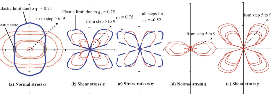
plane.

Fig. 12shows the distribution of local stresses and strains in rose diagrams for the ending step 4 of the first loading stage and the selected steps 5, 6, 7, 8, and 9 for the second loading stage (seeFig. 5a

-15 -10 -5 0 5 10 15 20

1 10 100

p' (kPa)

v

(%)

CAD 2443 =0.51 CAE 2529 =-0.26 CAE 2522 =-0.52

Simulation

Clay deposition history Previous consolidation

i =0.75

0

5

10

15

20

-10 -5 0 5 10 15

d (%)

v

(%

)

CAD 2443 =0.51 CAE 2529 =-0.26 CAE 2522 =-0.52

Simulation 0 2 4 6 8

10 30 50 70 90

p' (kPa)

v

(%)

CAD 2443 =0.51 CAE 2529 =-0.26 CAE 2522 =-0.52

Yield point Experiments = 0.51 = -0.52 0 2 4 6 8

10 30 50 70 90

[image:15.595.110.491.84.351.2]

p' (kPa) v (%) Simulations CAD2443 CAE2522 CAD2429 Yield point = 0.51 = -0.52

a

b

d

c

Fig. 10. Model prediction for tests with stress ratiogsmaller than that of previous consolidation stageg1.

-0.02 -0.01 0 0.01 0.02

0 0.02 0.04 0.06

(Mpa) (MP a) 18o 28o 45o 72o 55o (a) 90o 0o

1st loading stage 1 = 0.75

= -0.52 18o 28o 45o 72o 55o CAE2522 -0.02 0 0.02 0.04 0.06

0 0.02 0.04 0.06

(Mpa) 28o 18o 45o 72o 55o (b) 0o 90o

1 = 0.75

= -0.52 0o 90o CAE2522 -0.02 0 0.02 0.04 0.06

-0.015 -0.01 -0.005 0

[image:15.595.70.538.398.573.2]

18o 28o 45o 72o 55o (c) 0o 90o CAE2522

and b). It is noted that step 4 gives the pre-stresses on each contact plane at the end of first stage loading.

The distribution of normal stress at the end of the first loading stage (step 4) has a long axis in the vertical direction. During the sampling (4–40_{inFig. 5a and b), the distribution shrinks to the point of} origin as an unloading process. Then, it expands again during the second loading stage from step 5 to 9, but with a different shape that has the long axis in the horizontal direction (seeFig. 12a). The change in shape of the distribution is due to the load pattern, changing from compression to extension (from

g

1= 0.75 to

g

2=0.52).

At step 6 of the second stage, the distribution reaches the bold line only for planes with near-hor-izontal orientations. Only these planes, after reaching their pre-consolidation pressures, begin to behave plastically. At steps 7, 8, and 9 the number of planes that reached their pre-consolidation stress (i.e., went beyond the bold line) continues to increase. At step 9, there are still nearly half of the planes which behave elastically, which is consistent with Fig. 11b which shows that all the contact planes with less than 45°orientation did not yield. Thus, the soil has a smooth transition zone when it begins to yield in the curveev–logp0, as shown inFig. 10a, making it more difficult to define the apparent yield point based solely on globally applied stresses. It demonstrates that in this case, the first contact plane yields long before the apparent yield point determined from the bilinear construction, while many contact planes are still in the elastic state after the apparent yield point.

[image:16.595.65.535.76.244.2]

This case also shows that, due to a change of the loading path direction, the shape of the normal stress distribution can rotate around its principal axis, which indicates that the induced anisotropy involves not only the degree of anisotropy but also the axis of anisotropy.

Fig. 12b shows the distribution of shear stress andFig. 12c shows the distribution of shear to nor-mal stress ratio

s

/

r

, which governs the shear deformation. The distributions show that after the sec-ond loading stage, there are a small number of contact planes (below 45°orientation) which exceed the elastic limits created by the first loading stage.

Fig. 12d shows the distribution of local normal strains which indicates very small strains for con-tact planes having an orientation below 45°. For orientations greater than 45°, however, the planes display large normal strains due to their exceeding of the local elastic limit at early steps during this loading stage.Fig. 12e shows the shear strain distribution for the steps 6, 7, 8, and 9 of the second loading stage. The magnitude of shear strains is relatively small because most of the contacts are still in the elastic range at step 9.

3.3.3. Case 3:

g

2>

g

1

Three selected consolidation tests (Series C inTable 2) are considered in this case. After an identical first loading path

g

1= 0.11, three different second loading paths occurred are followed

g

2= 0.36, 0.58,

and 0.83 as shown in Fig. 13. Simulation for each test includes, sequentially, the clay deposition

g

0= 0.75, the first stage loading

g

1= 0.11 and the second stage loading

g

2. Particular attention was

given to the second loading stage. Fig. 14a shows theev–logp0 curves, and Fig. 14b theev–ed plane.

(a) Normal stress

Elastic limit due to 1 = 0.75

from step 5 to 9 Plastic state

(b) Shear stress

Elastic limit due to 1= 0.75

from step 5 to 9

(c) Stress ratio

1 = 0.75

all steps for

2 = -0.52

(d) Normal strain

from step 5 to 9

(e) Shear strain

from step 5 to 9

Similar to case 2, an obviously smooth transformation zone was found on theev–logp0plane, when the pre-consolidation stress was located. The apparent yield points determined from plots using a bilinear construction method are shown in the

e

v–p0 plane inFig. 14c and d.

Among the three tests,

g

2= 0.83 was selected for studying the contact planes. Fig. 15shows the

local stress–strain relationships for the contact planes in the selected orientations. In Fig. 15a, the

s

–

r

curves are plotted for both the first and the second loading stages. The slopes of the

s

–

r

curves for the second loading stage (

g

2= 0.83) are much higher than those for the first loading stage

(

g

1= 0.11).

In the local normal stress–strain curves, at the second loading stage (Fig. 15b), the elastic limits were reached for all planes except for the plane oriented at 90°. The magnitude of the normal stress decreases with the orientation angle caused by the stress distribution. In the local shear strain versus normal strain curves (Fig. 15c), the magnitude of local shear strain is greater for stress paths with higher slopes in the

r

–

s

plane. It is also noticeable that the shear strain in this case is larger than in the previous two cases.

Fig. 16shows the distribution of local stress and strain in rose diagrams for step 4 of the first load-ing stage and the selected steps 5, 6, 7, 8, and 9 for the second loadload-ing stage (Fig. 5a and b). The bold

p'

q

1 = 0.11

2 = 0.83

2 = 0.58

2 = 0.36

p'

q

1 = 0.11

2 = 0.83

2 = 0.58

[image:17.595.216.386.76.198.2]

2 = 0.36

Fig. 13. Schematic plot of drained constantgtests forg2>g1.

-15

-10

-5

0

5

10

15

1 10 100

p' (kPa)

v

(%)

CAD 2424 =0.83 CAD 2423 =0.58 CAD 2422 =0.36 Simulation

Clay deposition

1st loading stage

1 =0.11

2nd loading stage

0

5

10

15

20

0 5 10 15 20 25

d (%)

v

(%

)

CAD 2424 =0.83 CAD 2423 =0.58 CAD 2422 =0.36 Simulation

0

2

4

6

8

10 30 50 70 90

p' (kPa)

v

(%)

CAD 2424 =0.83 CAD 2423 =0.58 CAD 2422 =0.36

Yield point

Experiments

= 0.36

= 0.83

0

1

2

3

10 30 50 70

p' (kPa)

v

(%)

Simulations

CAD2422

CAD2424

Yield point

= 0.36

= 0.83 CAD2423

a

c

d

[image:17.595.113.489.258.517.2]

b

line shows the stresses at step 4 at the end of the first loading stage, which also represents the elastic limits for the second loading stage.

Corresponding to the near isotropic consolidation of the first loading stage (

g

1= 0.11), the bold line

has a shape close to a circle with its long axis in the vertical direction. The distribution of the second loading stage (

g

2= 0.83), however, has a shape much elongated in the vertical direction (Fig. 16a).

When distribution starts to expand from origin during the second loading stage, it reaches the bold line (elastic limits) at first for planes with near-vertical orientations at step 6. At steps 7, 8, and 9, the distribution expands further beyond the bold line. At the end of step 9, all planes yield, except for the planes with orientations near 90°, which is consistent withFig. 15b showing that all contacts yield except for the one with a 90°orientation. The yielding process is also stretched over several load steps, thus the soil has a smooth transition zone when it begins to yield in theev–logp0, as shown in Fig. 14a. It can be concluded that for the case of changing stress paths (stress path with various suc-cessive slopes

g

), the yielding condition does not occur simultaneously for all contact planes. There-fore, determining the yielding point from the test results at the macroscopic level becomes more difficult. This case also confirms that loading with reorientation of the stress path induces a change in the degree of anisotropy as well as in the direction of the anisotropy axis.

The fact that yielding condition does not occur simultaneously for all contact planes is a fundamen-tal phenomenon for granular material. In fact, the result can be used to explain the incremenfundamen-tally non-linear character of the material. As pointed out by many authors (Hill, 1965, 1966, 1967; Zienkiewicz and Pande, 1977; Bazant and Gambarova, 1984; Darve and Nicot, 2005), the mechanical state (elastic or plastic regime) of each contact depends on both the direction of the macroscopic loading and the orientation of the contact considered. As a consequence, the overall response corresponds to the

(a) Normal stress

Elastic limit due to

1 = 0.11

from step 5 to 9

Plastic state

(b) Shear stress

Elastic limit due to

1 = 0.11

from step 5 to 9

(c) Stress ratio

all steps for

2 = 0.83 Elastic limit due to

1 = 0.11

(d) Normal strain

from step 5 to 9

(e) Shear strain

[image:18.595.57.536.79.245.2]

from step 5 to 9

Fig. 16. Schematic plot for induced anisotropy forg2= 0.83.

-0.01 0 0.01 0.02 0.03

0 0.02 0.04 0.06 0.08

(Mpa)

(MP

a) 18

o 28o 45o

72o 55o

(a)

90o

0o 1st loading stage 1 = 0.11

= 0.83

CAD2424

Highest ratio 45o

-0.02

0

0.02

0.04

0.06

0 0.02 0.04 0.06 0.08

(Mpa)

28o 18o 45o 72o

55o

(b)

0o 90o

1 = 0.11

= 0.83 0o 90o

CAE2424

-0.02

0

0.02

0.04

0.06

-0.005 0 0.005 0.01 0.015

18o 28 o

45o 72o

55o

(c)

0o 90o

CAD2424

[image:18.595.72.519.293.451.2]

contribution of the individual response of all the contact directions. A very complex, nonlinear and anisotropic behaviour is therefore obtained.

Fig. 16b shows the distribution of shear stress andFig. 16c shows the distribution of shear to nor-mal stress ratio

s

/

r

. The distributions show that after the second loading stage, all planes exceed their shear elastic limits.

Fig. 16d shows the distribution of local normal strains which indicates very small strains for con-tact planes with near-horizontal orientation. Concon-tact planes with near-vertical orientations, however, display large normal strains due to their stresses beyond the initial elastic limits.Fig. 16e shows the shear strain distribution for steps 6, 7, 8, and 9 of the second loading stage. The magnitude of shear strains is relatively larger than in the previous two cases (seeFig. 15c) because the shear elastic limit is exceeded in contact planes of all orientations.

3.4. Investigating the macro apparent yield curve

As described in the previous section, the yield point is only an approximate description of the stress state, which serves as the elastic/plastic boundary for the material. Since the material cannot change its behaviour from elastic to plastic abruptly (i.e., contact planes are likely to yield in a sequential pro-cess), the yield point can be only approximately defined. The method used for determining the approximate yield point is a bilinear construction. In this section, the same method is used to con-struct the yield curve in a stress plane, as well as its kinematic rule based on the simulation of triaxial drained tests with different

g

-stress paths for the Otaniemi natural clay.

3.4.1. Initial apparent yield curve

In order to investigate the apparent yield curve of Otaniemi natural clay under clay deposition, drained tests of all series were simulated using the calibrated model parameters.Figs. 17 and 18show the comparison between experimental results and model predictions for the full range of test stages for Series A and B–C, respectively. A general agreement was achieved for all test simulations compared to experiments. The under-prediction of volumetric strains during the first loading stage at high val-ues of

g

(e.g., CAD2260, CAD2464, CAD2261), as noted byWheeler et al. (2003), can be attributed to the breakage of bonds among the clay clusters, which is not considered in the present microstructural model.

The apparent pre-consolidation pressures were measured by the bilinear method for all stress paths of the first loading stage. The initial apparent yield curve of Otaniemi natural clay in the nor-mally consolidated region was then obtained, as shown inFig. 19a. Considering the sample variability, the experimental data are scattered around the predicted results. The yield curve constructed from the results of the numerical simulations is approximately an elliptical shaped curve with a highest value of the mean effective stress lying approximately on the line

g

= 0.75.

3.4.2. Kinematic hardening of the macro apparent yield curve

As investigated in the previous section, a change of stress history (

g

2–

g

1) would redistribute the

local stresses and strains, resulting in a change of the anisotropy axes. In a conventional plasticity model, the change of the anisotropic axes would be reflected by a change of the yield surface shape, and would require a kinematic hardening rule to model such behaviour.

Drained tests with different

g

stress histories were simulated to construct the kinematic hardening of the yield curve. The

g

value of the first loading stage varies from 0.98 to0.34, using tests of Series B for

g

1= 0.75 along natural deposition stress path, CAD2260 for

g

1= 0.98, Series C for

g

1= 0.11,

CID2515 for

g

1= 0 and CAE2496 for

g

1=0.34. All tests were simulated by the microstructural model,

as shown in Figs. 17 and 18. General agreement was achieved for the experimental and numerical results.

Fig. 19b–f shows the apparent yield surfaces for different consolidation histories described by the microstructural model. All yield curves have different shapes, which are approximately of ellip-tical type with a highest value of the mean effective stress lying approximately on the line of the

g

1 stress path. In Fig. 19b, the stress path of the first loading stage is the same as that of the clay

the same shape. Fig. 19c–f shows cases with

g

1–

g

0. After the stress path

g

1 is applied, the yield

surface has not only moved but also changed its shape. The change in shape depends on the value of

g

1. The data plotted in Fig. 19b–f, corresponding to the final yield surface, are obtained from the

second loading stage in the test series. The constructed yield surfaces are compared to experimen-tal results, when available, as shown in Fig. 19a–f. Considering the soil variability, the comparison shows a reasonably good agreement. The micromechanical approach seems capable of describing adequately the kinematic hardening of a yield curve in the stress space.

4. Summary and conclusion

A microstructural model for clay based on the approach proposed by Chang and Hicher (2005) has been used to simulate the multistage drained constant –

g

tests on Otaniemi clay. The pur-pose of this study was to investigate the induced anisotropy due to various combinations of stress paths. It was attempted to link the mechanisms at inter-cluster contacts to the apparent

0 5 10 15 20 25 30 35 10 100 Exp. Model v (% ) p' (kPa) CAD2260

1 = 1.08

2 = 0.1

0 5 10 15 20 25 30 35 10 100 v (% ) p' (kPa) CAD2464

1 = 0.89

2 = 0.1

0 5 10 15 20 25 30 35 10 100 v (% ) p' (kPa) CAD2261

1 = 0.79

2 = 0.1

0 5 10 15 20 25 30 35 10 100 v (% ) p' (kPa) CAD2530

1 = 0.6

2= 0.32

0 5 10 15 20 25 30 35 10 100 v (%) p' (kPa) CAD2251

1 = 0.6

2= 0.09

0 5 10 15 20 25 30 35 10 100 v (%) p' (kPa) CAD2280

1 = 0.51

2= 0.1

0 5 10 15 20 25 30 35 10 100 v (%) p' (kPa) CAE2586

1 = 0.43

2= 0.51

0 5 10 15 20 25 30 35 10 100 v (%) p' (kPa) CAD2276

1 = 0.26

2= 0.11

0 5 10 15 20 25 30 35 10 100 v (%) p' (kPa) CAD2514

1 = 0.21

2= 0.74

0 5 10 15 20 25 30 35 10 100 v (%) p' (kPa) CAE2496

1 = -0.34

2= 0.1

0 5 10 15 20 25 30 35 10 100 v (%) p' (kPa) CAE2544

1 = -0.6

2= 0.51

0 5 10 15 20 25 30 35 10 100 v (%) p' (kPa) CAE2513

1 = -0.65

[image:20.595.55.532.74.541.2]

2= 0.61

0 5 10 15 20 25 30 35 10 100 Exp. Model v (% ) p' (kPa) CAD2443

1 = 0.75

2= 0.51

0 5 10 15 20 25 30 35 10 100 v (% ) p' (kPa) CAD2425

1 = 0.75

2= 0.22

0 5 10 15 20 25 30 35 10 100 v (% ) p' (kPa) CAE2529

1 = 0.75

2= -0.26

0 5 10 15 20 25 30 35 10 100 v (% ) p' (kPa) CAE2522

1 = 0.75

2= -0.52

0 5 10 15 20 25 30 35 10 100 Exp. Model v (% ) p' (kPa) CAD2423

1 = 0.11

2= 0.58

0 5 10 15 20 25 30 35 10 100 v (% ) p' (kPa) CAD2422

1 = 0.11

2= 0.36

0 5 10 15 20 25 30 35 10 100 v (% ) p' (kPa) CAD2561

1 = 0.11

2= -0.45

0 5 10 15 20 25 30 35 10 100 v (% ) p' (kPa) CAD2550

1 = 0.11

[image:21.595.62.542.79.397.2]

2= -0.58

Fig. 18. Model predictions on drained tests Series B and C.

-10 0 10 20

0 10 20

p' (kPa) q ( kPa ) CSL CSL

0 = 0.75

Exp. Series A

Model Initial yield curve

Initial 0 = 0.75

-20 0 20 40

0 20 40

p' (kPa)

q (

kPa

)

Exp.

Series B Model

= 0

0= 0.75

= 0.75

-20 0 20 40

0 20 40

p' (kPa) q ( kP a) Exp. CAD2260 Model

> 0

0 = 0.75

= 0.98 -40 -20 0 20 40

0 20 40 60

p' (kPa) q ( kPa ) Exp. Series C Model < 0

0 = 0.75

1 = 0.11

-40 -20 0 20 40

0 20 40 60

p' (kPa)

q (

k

Pa

) Exp. CID2515

Model

0 = 0.75

< 0

= 0 -20 -10 0 10 20

0 10 20 3

p' (kPa) q ( kPa ) Exp. CAE249 0 Model

0 = 0.75

< 0

= -0.34

a

b

c

f

e

[image:21.595.69.537.420.759.2]

d

yield surface and its kinematic hardening in the stress space. Three different cases have been studied:

(1) For the case

g

1=

g

0, thee–logp0curve for the first loading stage is bilinear and the yield point is

obviously situated at the intersection point of the two lines. When the applied stress reaches the pre-consolidation stress, all contact planes reach their pre-consolidation pressures simulta-neously, and therefore they all begin to behave plastically.

(2) For the cases

g

2<

g

1 and

g

2>

g

1, the e–logp0 curve for the second loading stage is no longer

bilinear, instead there is a smooth transition zone. In this case, the apparent yield point is deter-mined by the bilinear construction method proposed by Mitchell (1970). When the applied stress reaches the pre-consolidation stress, not all contact planes reach their pre-consolidation pressures simultaneously. The number of yield contacts increases with applied load but some contacts are likely to remain elastic. The cause of this phenomenon is easily detected from the evolution of the local stress distribution for contacts of various orientations.

It can be concluded that for the case of stress paths with various successive directions, the yielding condition does not occur simultaneously for all contact planes. Therefore, the definition of yield becomes vague for the traditional plasticity theory, where the yield point occurs at a given applied stress.

It can also be concluded that, due to a change of loading path, the principal axis of the contact stress distribution can rotate, which indicates that the induced anisotropy includes not only the degree of anisotropy but also the principal axes of anisotropy.

Under the microstructural approach, the evolution of the state variables (local stress and strain) in the planes of all orientations is tracked. This leads to an account of anisotropy on stress-dependent properties, and can produce naturally the anisotropic behaviour without specifying a kinematic hard-ening yield surface in the stress space.

Given the good agreement between the numerical simulation and the experimental results, the micromechanical approach seems capable of modelling adequately the induced anisotropic behaviour of Otaniemi clay.

Acknowledgements

The work presented here was sponsored in part by the Academy of Finland (Grant 210744) and car-ried out as part of a Marie Curie Research Training Network ‘‘Advanced Modelling of Ground Improve-ment on Soft Soils (AMGISS)” supported by the European Community through the programme ‘‘Human Resources and Mobility”. The writers would like to thank Matti Lojander at the Laboratory of Soil Mechanics and Foundation Engineering of Helsinki University of Technology, for his support.

References

Batdorf, S.B., Budianski, B., 1949. A mathematical theory of plasticity based on concept of slip. NACA Tech Note TN 1871. Bazant, Z.P., Gambarova, P.G., 1984. Crack shear in concrete: crack band microplane model. ASCE Journal of Structural

Engineering 110 (9), 2015–2035.

Bazant, Z.P., Xiang, Y., Ozbolt, J., 1995. Nonlocal microplane model for damage due to cracking. Proceedings of Engineering Mechanics 2, 694–697.

Biarez, J., Hicher, P.Y., 1994. Elementary Mechanics of Soil Behaviour. Balkema. pp. 208.

Burland, J.B., 1990. On the compressibility and shear strength of natural clays. Geotechnique 40 (3), 329–378. Calladine, C.R., 1971. Microstructural view of the mechanical properties of saturated clay. Geotechnique 21, 391–415. Chang, C.S., Gao, J., 1995. Second-gradient constitutive theory for granular material with random packing structure.

International Journal of Solids and Structures 32 (16), 2279–2293.

Chang, C.S., Hicher, P.Y., 2005. An elastic–plastic model for granular materials with microstructural consideration. International Journal of Solids and Structures 42, 4258–4277.

Chang, C.S., Liao, C., 1990. Constitutive relations for particulate medium with the effect of particle rotation. International Journal of Solids and Structures 26, 437–453.

Chang, C.S., Sundaram, S.S., Misra, A., 1989. Initial moduli of particulate mass with frictional contacts. International Journal for Numerical and Analytical Methods in Geomechanics 13 (6), 626–641.