An HEI-disaggregated input-output table for Scotland

S

TRATHCLYDE

DISCUSSION PAPERS IN ECONOMICS

DEPARTMENT OF ECONOMICS

UNIVERSITY OF STRATHCLYDE

GLASGOW

AN HEI-DISAGGREGATED INPUT-OUTPUT TABLE FOR

SCOTLAND

BY

KRISTINN HERMANNSSON, KATERINA LISENKOVA,

PETER G. MCGREGOR AND KIM SWALES.

An HEI-Disaggregated Input-Output Table for Scotland*

Kristinn Hermannsson

Katerina Lisenkova

Peter G. McGregor

and

J. Kim Swales

Fraser of Allander Institute, Department of Economics,

University of Strathclyde

September 2010

Abstract

This paper describes how the education sector of the Scottish Input-Output tables is

disaggregated to identify a separate sector for each of Scotland’s twenty Higher

Education Institutions (HEIs). The process draws on accounting and survey data to

accurately determine the incomes and expenditures of each institution. In particular

we emphasise determining the HEIs incomes source of origin to inform their treatment,

as endogenous or exogenous, in subsequent analyses. The HEI-disaggregated

Input-Output table provides a useful descriptive snapshot of the Scottish economy and the

role of HEIs within it for a particular year, 2006. The table can be used to derive

multipliers and conduct various impact studies of each institution or the sector as a

whole. The table is furthermore useful to calibrate other multi-sectoral,

HEI-disaggregated models of regional economies, including Social Accounting Matrix

(SAM) and computable general equilibrium (CGE) models.

Keywords: Higher Education Institutions, Universities, Input-Output, Scotland, Impact

study, Multipliers, Devolution.

4

1. Introduction

In this paper we explain how we augment official Input-Output tables to construct

an HEI-disaggregated Input-Output table for Scotland. Within this table each

Higher Education Institution (HEI) in Scotland is represented as a separate sector

with its own row, detailing its income structure, and its own column for its

expenditures. The HEI-disaggregated Input-Output table provides a useful

descriptive snapshot of the Scottish economy, and the role of HEIs within it for a

particular year, 2006. The table can also be used to calibrate a conventional

input-output model that enables the derivation of, for example, input-output, value-added

and employment multipliers for each higher education institution, as well as for the

HEI sector as a whole. Furthermore, the table facilitates a wide range of additional

Input-Output based “impact” studies, and may also be used in attribution analyses.

The Input Output table is, in addition, an essential component of databases used to

calibrate other multi-sectoral, HEI-disaggregated models of regional economies,

including Social Accounting Matrix (SAM) and computable general equilibrium

(CGE) models.

To our knowledge this is the first example of an Input-Output table that treats each

Scottish HEI as a separate sector in a single unified framework. We do not apply

universal assumptions to all HEIs, but rather seek to determine incomes and

expenditures individually for each in a coherent and transparent manner1_{. This}

enables the first consistent comparison of the expenditure effects of individual HEIs

in Scotland. To a significant degree we can determine the income and

expenditure structure of each HEI from accounting data relating to each institution,

by drawing on databases provided by the Higher Education Statistics Agency

(HESA). In addition we employ survey data and purchasing data from the Joint

Consultative and Advisory Committee on Purchasing (JCAPC), the purchasing

consortium of HEIs in Scotland and Northern-Ireland. Nevertheless, we have to

make some general assumptions in respect of a number of elements of incomes

1 _{The Input-Output table is a natural extension of the work undertaken by Iain McNicoll,}

5

and expenditures. While these impact on a relatively small part of the relevant

totals, we endeavour to be as transparent as possible, so that other researchers

may scrutinise our assumptions, and perhaps choose to modify them, in future

expenditure analyses of Scottish HEIs.

The paper is structured as follows. In Section 2 we explain how the

HEI-disaggregated Input-Output table is constructed. In Section 3 we present an

aggregated version of the table, and some summary descriptive statistics and

multipliers for individual sectors and HEIs, the derivation of which is explained in an

Appendix. Finally, in section 4, we present brief conclusions.

2.

Construction of an HEI-disaggregated Input-Output table

Our chosen reference year is 2005/2006 since this is the latest year for which the

necessary data were available. The procedure used to derive the HEI

disaggregated IO-table can be divided into two steps. First we “rolled forward” the

2004 Scottish IO table to reflect changes in Gross Value Added (GVA) from 2004 to

2006. We then create an individual row and column for each institution.

2.1

Rolling forward the 2004 IO table

Since the academic year 2005/2006 has been chosen as the reference year of the

study, the official Scottish analytical I-O Table for 2004 (Scottish Government, 2007)

had to be rolled forward to reflect the output level and prices in the year 2006. This

is done using Gross Value Added (GVA) as a benchmark. Between 2004 and 2006

GVA increased by 10.28% from £82,538 million to £91,024 million. All of the figures in

the official 2004 table are uniformly adjusted upwards by a factor of 1.1028.

Comparisons of surveyed IO tables have shown that changes in the technical

structure of an economy occur slowly so that limited change can be expected

over the short run (Miller & Blair, 2009). Accordingly, extrapolating the table to

reflect price and volume changes over a two-year period is unlikely to result in

significant errors. Furthermore, the analysis can be updated in due course to assess

6

2.2

Disaggregation of the Education Sector

The next step is to separate out the HEIs’ sector from the education sector as a

whole, which corresponds to IO sector code 116 in the official Scottish IO accounts.

The additional data required are sourced from HESA (2007a), which gives

information on output totals and expenditure on wages. In addition, data on

income by source can be used to estimate exports for each institution. By

combining income and expenditure totals from HESA with accounting and survey

data on HEIs’ expenditures we are able to construct a separate row and column

for each institution. Finally, the individual HEI rows and columns are summed and

then deducted from the education sector in the IO table to form an Education

sector that excludes HEIs.

2.2.1

Creating separate columns for each HEI

A column in an IO table reveals the total expenditure of a sector and how it is

divided between intermediate inputs, imports and valued added. The following is a

description of the steps taken in creating a separate column for each HEI.

The first issue is the estimation of imports for each institution. We have data on the

amount of interregional and international imports from JCAPC, the purchasing

consortium for Scottish and Northern Irish HEIs. These data reveal aggregate

expenditures by Scottish HEIs broken down by category and geographic location

of suppliers (Scottish, rest of UK (RUK), overseas). Imports were 12.9% of total output

in 2005/2006. Ninety eight per cent of total imports come from RUK and only 2% are

international imports, so that the interregional links predominate. The data do not

reveal purchases of individual HEIs so the proportions are applied uniformly to all of

them. This import propensity differs from ones assumed in previous impact studies.

For example (Kelly 2004) assume 25% while (Harris 1997) calculates imports to be

22% based on the narrow geographic definition of Portsmouth. Input-Output tables

for Scotland record imports to the education sector at 11% of the value of total

7

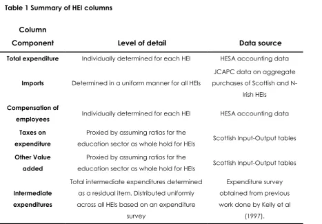
Table 1 Summary of HEI columns

Column

Component Level of detail Data source

Total expenditure Individually determined for each HEI HESA accounting data

Imports Determined in a uniform manner for all HEIs

JCAPC data on aggregate

purchases of Scottish and

N-Irish HEIs

Compensation of

employees Individually determined for each HEI HESA accounting data

Taxes on

expenditure

Proxied by assuming ratios for the

education sector as whole hold for HEIs Scottish Input-Output tables

Other Value

added

Proxied by assuming ratios for the

education sector as whole hold for HEIs Scottish Input-Output tables

Intermediate

expenditures

Total intermediate expenditures determined

as a residual item. Distributed uniformly

across all HEIs based on an expenditure

survey

Expenditure survey

obtained from previous

work done by Kelly et al

(1997).

From HESA publications we have data on employment costs (compensation of

employees) and total output (income) by source. The remaining elements of each

IO column we need to derive are: the intermediate purchases, net taxes and gross

operating surplus. Net taxes and gross operating surplus were determined for each

HEI as the same proportion of overall expenditure as in the education sector as a

whole (IO116) in the 2004 tables. These represent a small fraction of overall

expenditure: 2.8% for net taxes, and 3.1% for gross operating surplus.

Having identified all of the other cost elements the residual is the amount of

intermediate purchases from Scottish industries. The sectoral distribution of this

expenditure was governed by the coefficients used by Kelly et al (2004). These

coefficients of intermediate expenditures are based on a survey of UK HEIs

described in Kelly et al (1997). Production technology in IO tables has been found

to change only very gradually (Miller & Blair, 2009). It is likely therefore that new

8

the composition of intermediate inputs; expenditure on intermediate inputs is less

than a quarter of the total output of HEIs (23% on average). In any case there was

no funding available for new survey work on HEIs in the current project, but this

could easily be revisited in future.

2.2.2

Creating separate rows for each HEI

A row in an IO table reveals the total income of a sector and the various

components of income, including intermediate sales to other production sectors

and sales to final demand sectors such as households, government and exports.

Table 2 summarises the methods and sources we used to identify individual HEI’s

revenues.

Table 2 Summary of HEI rows

Row Component Level of detail Data source

Income from exports Individually determined

for each HEI

Accounting data from HESA

Income from Scottish Government

Individually determined for each HEI

Accounting data from HESA

Income from other final demand categories and

intermediate demand

Income apart from exports and Scottish

Government funding is uniformly distributed along

the row based on proportions of the overall

education sector

Scottish Input Output table

Drawing on HESA data allows us to construct IO rows that reflect the particular

structure of each HEI’s income. HEI incomes from Exports and the Scottish

Government amount to 29% and 54% respectively of HEIs’ income on average.

These two categories alone represent 83% of the HEI sector’s total income and are

determined separately for each HEI based on HESA accounting data. This is a key

feature of the HEI-disaggregated IO table, which enables an accurate account of

the heterogeneity of HEIs’ income structures. The residual obtained by deducting

9

along the row (other final demand categories and intermediate demand) in the

same proportions as in the overall education sector (IO 116) of the Scottish

Input-Output tables.

HESA classifies HEIs’ income into broad categories and a number of subcategories.

We allocate these incomes to four distinct categories depending on whether they

come from the Scottish Government and whether they originate within or outwith

the Scottish economy. From the definitions of these sub-categories, 84% of HEIs

income can be attributed directly either to local demand (Scottish Government or

other demand) or export demand (RUK, ROW). The remaining 16% of HEIs income

categories constitute income originating from some combination of either local,

RUK or ROW sources, for which the exact proportions are unknown. In these cases

income is attributed indirectly based on the weights revealed by income sources

with a known and unambiguous origin. The details of how each of these

10

Table 3 Attribution of HESA income sources in IO table to origin – Scottish Government, rest of the UK (RUK), rest of the World (ROW) and other demand

Income category Attribution Total

Funding Council grants

Recurrent grants (Teaching)

Scottish Government

28%

Recurrent grants (Research) 9%

Recurrent grants (other) 3%

Release of deferred capital grants 1%

FE provision 0%

Tuition fees & education grants & contracts

Standard rates _{Attributed to ScotGov}

and RUK demand based on student numbers

8%

Non-standard rates 2%

Part-time HE fees 1%

Non-EU domicile ROW 7%

Non-credit bearing course fees

Other (local demand) 1%

Other fees & support grants 1%

Research grants & contracts

OSI Research Councils RUK 7%

UK based charities

Indirectly attributed

4%

UK central government/local authorities, health & hospital authorities 3%

UK industry, commerce & public corporations 2%

Other sources Other 0%

Other overseas sources

ROW 1%

EU sources 2%

Other income - other services rendered

UK central government/local authorities, health and hospital authorities, EU government bodies

Indirectly attributed 2%

Other 3%

Other income - other

Grants from local authorities Scot Gov 0%

Release of deferred capital grants

Indirectly attributed

1%

Income from health & hospital authorities (excluding teaching contracts for teaching provision) 1%

Income from intellectual property rights 0%

Residences & catering operations (including conferences) Student numbers 6%

Other operating income ROW 5%

Endowment & investment income Other 2%

11

In the remainder of this section we discuss the treatment of income

sources and the assumptions required to allow us to attribute all of HEIs’

income to IO demand categories. We begin by considering those

income categories that have a clear origin, and then discuss our

treatment of those that are more ambiguous.

Funding Council grants

The whole of the category ‘Funding Council Grants’ reports funding

provided by the Scottish Funding Council (SFC). This is ultimately drawn

from the Scottish block grant and hence attributed to the Scottish

Government.

Tuition fees & education grants & contracts

In the HESA dataset tuition fees are pooled for Scottish, RUK and REU

students. Student numbers by origin are used to disaggregate these into

Scottish, RUK and REU tuition fees. The Scottish Funding Council pays for

Scottish students. We treat the tuition fees of REU students as Scottish

Government demand under the assumption they are all Erasmus

exchange students, whom the Scottish Funding Council pays for as well.

RUK tuition income is treated as RUK exports. Tuition fees of students from

outwith the EU are treated as ROW exports. Non-credit bearing course

fees and Other fees & support grants represents courses that the HEIs

charge for and are therefore attributed to Other demand. HESA (2007a)

does not explicitly define the category Other fees & support grants. This

is assumed to be income from Other local demand.

Research grants & contracts

Research income from the OSI research councils2 _{is treated as RUK}

exports as these are funded by the central government of the UK. Other

overseas sources and EU sources are classed as ROW exports. Other

2 _{The category “OSI Research Councils“ refers to funding from the various}

12

sources are, for simplicity, assumed to come from other demand3 _Other

sub-categories under this heading are indirectly attributed (see

discussion below).

Other income – other services rendered

These income streams are for various services rendered, including

consultancy to external bodies both public and private, UK and foreign.

These are attributed indirectly (see further discussion below)

Other income – other

The category Other income – other is treated in three different ways

depending on the sub-category. Grants from local authorities are

attributed to the Scottish Government. This is a simplifying assumption as

only a part of Scottish local Government’s incomes are derived from the

Scottish Government and the Scottish block grant. Residence &

catering operations mainly comprises student residences and

on-campus catering services consumed by students. Therefore we use

student numbers by origin to attribute this income to local demand and

exports. Some of these services are consumed by conference

attendees. We assume that the ability of the university to attract

conference guests is proxied by the student population. Other

operating income is treated as ROW exports since, according to HESA

definitions, this mostly comprises European funding sources. Income from

intellectual property rights is for simplicity assumed to stem from other

local demands4_{. The remaining sub-categories are attributed indirectly.}

Indirectly attributed incomes

Seven HESA accounting categories, 16% of the total of HEIs’ income,

have an ambiguous spatial origin. Although we cannot directly

determine the origin of the various incomes that have to be attributed

indirectly, the definitions of the HESA accounting categories give some

3 _{This only contributes 0.34% of HEIs income and so is not a material}

concern.

13

indication of their nature. We try to capture this by devising an

attribution mechanism that is consistent with the nature of the income

category. The application of these is summarised in Table 3 and

described for each case below.

Research grants & contracts

Income from ‘UK based charities’ is from charities in either Scotland or

other UK regions. We expect the HEIs to draw mostly on local charities,

so we attribute this income category to Other local demands. However,

we allow for some export income from RUK in the same proportion as

the RUK export intensity of research income.

Income from UK central government/local authorities, health & hospital

authorities will by definition either originate from central government

funding at the UK level, in which case it will be counted as RUK-exports,

or from funding sources that can ultimately be traced back to the

Scottish block grant and hence will be attributed to the Scottish

Government. To determine the relative weight of each we use

non-student incomes as revealed by directly allocated income as a basis for

distribution to final demand.

UK industry, commerce & public corporations is assumed to originate

from other regions of the UK, in which case it is counted as exports, or

Scottish non-government sources (intermediate demand) in which case

it is attributed to other local demands. To determine the proportion that

is attributed to RUK-exports we use the RUK export intensity of research

incomes with known spatial origin (30%). We assume that the HEIs

predominantly interact with local producers and hence allocate the

remainder of this income to other local demands.

Other income – other services rendered

UK central government/local authorities, health and hospital authorities,

EU government bodies can in principle originate from both local and

14

Scottish production sectors, UK-consumers, EU-funding, etc,). We use

non-student income as revealed by directly attributed income sources

as a basis for distribution among final demand categories. This income

category includes income from non-departmental public bodies and

because of its services-rendered nature it is reasonable to assume some

of this is intermediate demand from Scottish production sectors (other

local demands), rather than attributing it solely to Scottish Government

demand and exports.

Income classed as ‘Other’ is assumed to originate either from

intermediate demand or exports. Again, we assume this income is

primarily raised locally except for RUK income, based on the RUK export

intensity as revealed by directly attributed income sources.

Table 4 Indirect attribution of incomes

Attributed to % of total

income

Scot

Gov RUK ROW Other

Research grants & contracts

UK based charities 4%

•

•

UK central government/local authorities, health &

hospital authorities 3%

•

•

UK industry, commerce & public corporations 2%

•

•

Other income - other services rendered

UK central government/local authorities, health

and hospital authorities, EU government bodies 2%

•

•

•

•

Other 3%

•

•

Other income - other

Release of deferred capital grants 1%

•

•

Income from health & hospital authorities (excluding teaching contracts for teaching provision)

1%

•

•

16%

15

Release of deferred capital grants comprises capital grants from sources

other than the higher education funding councils. We assume this can

involve local non-government sources as well as sources in RUK and

ROW (perhaps EU). We assume the pattern of this income source follows

that of the HEIs research income in general and use the previously

revealed origins of research income as a basis for distributing these

grants between other demands and RUK and ROW exports.

Income from health & hospital authorities (excluding teaching contracts

for teaching provision) can in principle derive from health and hospital

authorities either within Scotland (in which case they are ultimately

derived from the Scottish block grant) or the other regions of the UK (in

which case it will be treated as RUK exports). To determine the relative

weight of each we use non-student incomes as revealed by directly

allocated income as a basis for distribution to final demand.

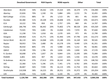
Table 5 Income of Scottish HEIs by origin, £m %

Devolved Government RUK Exports ROW exports Other Total

Aberdeen 85,018 54% 20,262 13% 25,324 16% 26,379 17% 156,983 100% Abertay 22,826 70% 1,530 5% 5,884 18% 2,215 7% 32,455 100% Bell College 17,551 88% 59 0% 1,513 8% 801 4% 19,924 100% Dundee 83,380 51% 24,109 15% 24,848 15% 31,635 19% 163,971 100% ECA 10,222 70% 858 6% 2,757 19% 869 6% 14,707 100% Edinburgh 186,796 43% 86,442 20% 73,802 17% 88,528 20% 435,569 100% Caledonian 73,925 76% 2,681 3% 13,064 13% 7,974 8% 97,644 100% GSA 11,238 71% 1,018 6% 2,570 16% 973 6% 15,799 100% Glasgow 160,862 51% 41,771 13% 41,943 13% 67,796 22% 312,372 100% Heriot-Watt 46,119 46% 14,068 14% 23,188 23% 16,169 16% 99,545 100% Napier 58,953 72% 2,680 3% 10,278 13% 9,440 12% 81,351 100% Paisley 46,910 80% 378 1% 5,980 10% 5,212 9% 58,481 100% QMUC 19,199 70% 1,706 6% 3,836 14% 2,830 10% 27,570 100% R. Gordon 50,008 67% 1,837 2% 9,844 13% 13,395 18% 75,084 100% RSAMD 6,801 66% 407 4% 1,613 16% 1,556 15% 10,378 100% St Andrews 40,216 37% 27,613 25% 28,342 26% 12,592 12% 108,762 100% SAC 22,360 51% 5,196 12% 7,341 17% 8,762 20% 43,659 100% Stirling 46,867 56% 7,928 9% 16,115 19% 12,754 15% 83,663 100% Strathclyde 110,508 58% 16,223 8% 28,351 15% 35,972 19% 191,054 100% UHI 25,026 71% 5,540 16% 3,220 9% 1,579 4% 35,365 100%

Total Scotland 1,124,784 54% 262,306 13% 329,813 16% 347,433 17% 2,064,336 100%

The calculated exports and Scottish Government incomes directly enter

16

coefficients of the Education sector from the existing IO table to

distribute other income between other categories of final demand and

intermediate income from other sectors for each institution. This

concludes the procedure of estimating the IO rows for each institution.

Having derived columns and rows for each HEI we next incorporate

them into the existing (rolled forward) Input-Output table. The estimated

rows and columns are subtracted from the existing “Education” sector.

The resultant IO table has 148 sectors of which 20 represent the higher

education institutions themselves.

2.3

Sectoral employment

Sectoral full-time-equivalent (FTE) employment figures are based on

those published in the 2004 Scottish IO tables. Since the base year is

2006 these had to be updated. For this we use head count data from

the Annual Business Inquiry, which reports full time and part time

employment by region. Following convention, part time employment

was divided by 3 to approximate full time equivalence. Comparing

headcount figures for 2004 and 2006 reveals an employment growth of

1.4%, which was used to update the FTE employment level. Employment

in the HEIs is reported in Table 25 of HESA (2007), which reveals FTE

employment of all staff of each HEI for the academic year 2005/2006.

2.4

Student numbers

Student numbers are used to disaggregate UK tuition fees by their origin

from within Scotland or from other UK regions (RUK). Furthermore, in

subsequent applications of the IO-tables, for calculating the economic

impact of HEIs, student numbers are used to inform the estimation of

students’ consumption impact. The published student numbers in HESA

(2007b) do not provide sufficient detail on the spatial origin of the

17

their student records database, which provided us with FTE student

numbers disaggregated by origin from each of the UK regions (England,

N-Ireland, Scotland and Wales), the EU, the rest of Europe and the rest of

the World. For the purpose of constructing the IO-table the student

population of each institution is aggregated into three groups, Scottish

students (SCO), students from the rest of the UK (RUK) and students from

the rest of the World (ROW). A summary of these is provided below.

Table 6 Student numbers by origin at Scottish HEIs (FTEs, %)

SCO RUK ROW Total

Aberdeen 7,749 70% 1,557 14% 1,774 16% 11,079 100%

Abertay 2,704 72% 278 7% 749 20% 3,731 100%

Bell College 3,067 99% 19 1% 4 0% 3,091 100%

Dundee 9,462 72% 1,810 14% 1,868 14% 13,140 100%

ECA 799 49% 379 23% 442 27% 1,620 100%

Edinburgh 9,495 46% 7,201 35% 3,745 18% 20,440 100%

Caledonian 12,466 88% 629 4% 1,054 7% 14,149 100%

GSA 789 53% 423 28% 289 19% 1,501 100%

Glasgow 14,267 76% 2,360 13% 2,145 11% 18,773 100%

Heriot-Watt 3,859 55% 1,276 18% 1,892 27% 7,027 100%

Napier 6,627 70% 675 7% 2,220 23% 9,522 100%

Paisley 6,940 90% 114 1% 661 9% 7,716 100%

QMUC 2,648 66% 549 14% 817 20% 4,013 100%

Robert Gordon 7,121 76% 395 4% 1,867 20% 9,383 100%

RSAMD 439 65% 135 20% 105 15% 678 100%

St Andrews 2,370 33% 2,512 35% 2,245 31% 7,128 100%

SAC 603 89% 46 7% 26 4% 675 100%

Stirling 5,344 75% 1,011 14% 811 11% 7,165 100%

Strathclyde 13,913 86% 611 4% 1,729 11% 16,253 100%

UHI 3,599 95% 72 2% 114 3% 3,785 100%

18

3.

The Scottish HEIs sector and the Scottish economy

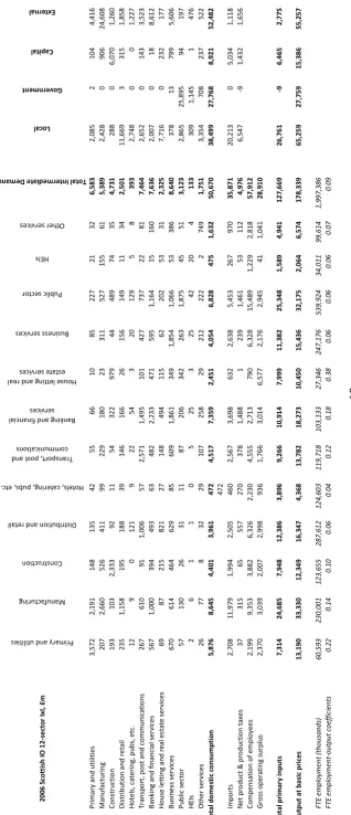
In this section we draw on the HEI-disaggregated Input-Output table

and some of the data sources used in its construction to describe the

characteristics of the HEIs sector within the context of the Scottish

economy. Although the table was constructed at a 148 sector level of

aggregation it is presented in a condensed 12-sector format below to

simplify the presentation. We explain how we compute the multipliers

reported in this section of the paper in an Appendix.

Based on the HEI disaggregated IO-table we can obtain the broad

characteristics of Scottish HEIs. Their relatively small type I multipliers

reflect the fact that HEIs do not source much intermediate inputs locally,

or indeed elsewhere as their import propensity is also low (12.9%). Of the

12 sectors shown in the table below HEIs exhibit the highest Type II

multiplier indicating that local wages form a bigger share of expenditure

than in other sectors. This is evident from Figure 1 below.

Table 7: Output multipliers of IO sectors

Sector Type I Type II

Primary and utilities 1.72 2.10

Manufacturing 1.39 1.83

Construction 1.53 2.07

Distribution and retail 1.35 1.90

Hotels, catering, pubs, etc. 1.16 1.80

Transport, post and communications 1.48 2.03

Banking and financial services 1.59 1.96

House letting and real estate services 1.34 1.55

Business services 1.37 1.99

Public sector 1.30 1.97

HEIs 1.33 2.12

20

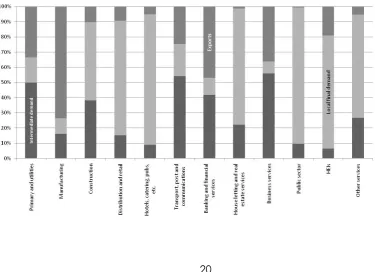
Figure 1: Expenditure structure of Scottish IO sectors

HEIs’ income is primarily driven by local final demand but just under a quarter of

their income is from exports. These characteristics set HEIs apart from the ‘public

sector’ which receives negligible income from final demand.

21

4. Conclusions

This paper explains how we augment the official IO tables to create an

HEI-disaggregated IO table for Scotland in 2006. We also present an aggregated

version of the table and some illustrative “multiplier” results. The purpose of this

paper is to furnish interested providers and users of HEI regional impact studies with

a publicly available, transparent account of how we create the database, and

identify areas where such data might be improved in future, through further survey

work for example.

Of course the main value of any database lies in the analyses that it allows us to

undertake. Firstly, in Hermannsson et al (2010a) we explore the “policy scepticism”

that has recently challenged the value of regional HEI impact studies. On the basis

of our database we are able to reject the extreme form of policy scepticism, which

asserts that HEI expenditure effects are negligible, for the HEI sector as a whole.

However, we also establish the importance of accounting for the regional public

sector budget constraint in regional economic impact analyses, at least within

devolved regions. Secondly, we extend our analysis to the expenditure impacts of

individual HEIs and their students in Hermannsson et al (2010b), in which the

heterogeneity of HEI expenditure impacts in Scotland is highlighted.

Thirdly, we are applying our approach to the expenditure impacts of HEIs in the

other devolved regions of the UK, namely Wales and Northern Ireland. Fourthly,

even though there is no regional budget constraint for England, it is nevertheless

instructive to explore the opportunity cost of the public funding of HEIs there, using

the approach developed in Hermannsson et al (2010a,b).

Fifthly, the regional databases can be developed into HEI-disaggregated

interregional IO tables that allow an analysis of the impact of HEIs’ expenditures on

non-host regions. Sixthly, drawing on additional income and expenditure data we

construct HEI-disaggregated social accounting matrices (SAMs), which we employ,

together with other supplementary data and analysis, to parameterise

HEI-disaggregated CGE models of regional economies. Such models allow us to

explore the system-wide, regional supply-side impacts of HEIs that operate through,

22

activities. In Hermannsson et al (2010c), for example, we employ an

HEI-disaggregated CGE model of Scotland to assess the contribution of graduates to

23

References

Harris, R. (1997), The Impact of the University of Portsmouth on the Local Economy.

Urban Studies, vol. 34, pp. 605-626.

Hermannsson, K., Lisenkova, K., McGregor, P. G and Swales, J. K. (2010a). ‘Policy

Scepticism’ and the Impact of Scottish Higher Education Institutions (HEIs) on the

Scottish Economy: Accounting for Regional Budget Constraints under Devolution,

Strathclyde Discussion Papers in Economics, 10-15.

Hermannsson, K., Lisenkova, K., McGregor, P. G and Swales, J. K. (2010b). The

Expenditure Impacts of Individual Higher Education Institutions (HEIs) and their

Students on the Scottish Economy under Devolution: Homogeneity or

Heterogeneity? Strathclyde Discussion Papers in Economics, 10-16.

Hermannsson, K., Lisenkova, K., McGregor, P. & Swales, J. K. (2010c). The

Importance of Graduates to the Scottish Economy: A “Micro-to-Macro” Approach,

Strathclyde Discussion Papers in Economics, forthcoming.

Higher Education Statistics Agency – HESA (2007a). Resources of Higher Education

Institutions 2005/06

Higher Education Statistics Agency – HESA (2007b). Students in Higher Education

Institutions 2005/06

Kelly, U., McNicoll, I & McLellan, D. (2004). The Impact of the University of

Strathclyde on the economy of Scotland and the City of Glasgow. Glasgow,

University of Strathclyde.

Kelly, U., McNicoll, I. & McCluskey, K. (1997). The Economic Impact of Universities

and Colleges on the UK Economy. London, CVCP.

McGregor, P., Swales, K. & Yin, Y.P. (1996). A long-run interpretation of regional

24

McGregor, P., Swales, K. & Yin, Y.P. (1999). Spillover and feedback effects in general

equilibrium interregional models of the national economy: a requiem for

interregional input-output? In Hweings, G., Sonis, M., Madden & Kimura, Y. (eds.)

Understanding and interpreting economic structure. Berlin: Springer Verlag.

Miller, R.E. & Blair, P.D. (2009), Input-Output Analysis: Foundations and Extensions,

second edition. Cambridge: Cambridge University Press.

Scottish Government – Riaghaltas na a h-Alba (2007) Input-Output Tables and

Multipliers for Scotland: Retrieved from the World Wide Web:

http://www.scotland.gov.uk/Topics/Statistics/Browse/Economy/Input-Output/IOAllFiles2004

Seafish (2007). The economic impacts of the UK sea fishing and fish processing

sectors: an Input-Output analysis. Report commissioned by Sea Fish Industry

25

Appendix. Input-Output tables, models and multipliers

A.1 Input-Output tables

Input-Output tables provide a snapshot of production in an economy for a given

year. They reveal the activities of industries that both produce goods (outputs) and

consume goods from other industries (inputs). The Input-Output tables are put to a

wide range of uses5 _{but are most frequently employed in various multiplier or}

“impact” analyses. Input-output models are calibrated using IO tables. Multipliers

are derived so that output is equal to the multiplier times the exogenous

components of demand, i.e. an explicit distinction is made between exogenous

and endogenous economic activity as we illustrate in section A.2. Here we briefly

describe the layout of Input Output tables and how they are split into exogenous

and endogenous components to derive multiplier values. We also show how

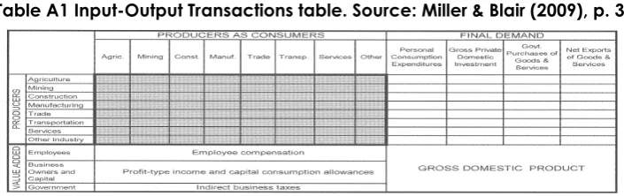
multipliers are defined and how they are interpreted6_.

Table A1 Input-Output Transactions table. Source: Miller & Blair (2009), p. 3

Input-Output tables provide a description of the flows of inputs and outputs to and

from production sectors in a particular year. A column in an Input-Output table

reveals the consumption (expenditures) of production sectors. The inter-industry

transactions table (shaded area) shows how each industry (reading down its

column) purchases inputs from within the same industry and from other industries.

The bottom part of the column shows the industry‘s expenditures on value added

such as employees, capital and government taxes. Reading the rows in the table

5 _{For details of Input-Output applications and methodology see Miller & Blair (2009).}

26

reveals the value of outputs sold by a particular industry to itself and to other

industries within the region and to final demand. The Input Output table is

consistent with national accounts. Adding up the final demand columns gives us

GDP by the expenditure method (C+I+G+(E-M)) and summing the value added

rows gives GDP by the factor income method7_.

A.2 Assumptions of Input-Output modelling

The underlying idea behind multipliers is that some independent (exogenous)

disturbance occurring in one part of the economy can have subsequent “knock

on” impacts in other parts of the economy and therefore on the economy as a

whole.

Demand-driven multipliers8 _{identify the impact of a sector as a purchaser of inputs.}

When a sector expands, it requires more inputs of intermediate goods and services

and increases its employment and wage payments. This generates positive

knock-on effects in sectors supplying the increased demand for intermediate and

consumption goods. The expansion in these sectors will produce further increases in

intermediate and consumption demands, the process continuing down successive

rounds of the multiplier process, with the additional impact in each successive

round becoming smaller and smaller. I-O analysis has a technique for capturing all

these effects, as long as a number of assumptions hold.

A key characteristic of the procedure for determining the demand-driven multiplier

values is to identify those elements of demand taken to be exogenous and those

taken to be endogenous. The exogenous elements are those that are determined

7 _{Note however that in Table 5 the Scottish Input-Output table is presented in a slightly}

different format where imports enter as part of primary inputs and in final demand we have gross exports as opposed to net-exports as in Table 7.

8 _{Two broad generic types of multiplier are identified in the I-O literature. These are}

27

independently of the level of activity within the economy. The endogenous

demands are those determined by the level of activity in the economy. In

conventional I-O demand-driven analysis, final demand, such as exports,

government expenditure, investment and stock building are exogenous.

Intermediate demand, including imports, is endogenous. Conventionally, we can

classify consumption expenditure as either exogenous or endogenous. This is

because it is not linked to production output through fixed production coefficients,

but through behavioural relationships that assert that domestic consumption will rise

in line with wage income.

When consumption expenditure is taken to be exogenous, the multiplier simply

identifies the change in activity generated in the economy by changes in

intermediate demand for goods and services. This multiplier is a Type I multiplier. It

consists of the direct effects of the initial change in exogenous demand plus the

indirect effects of the additional expenditure on intermediate goods and services.

Where consumption demand is endogenous, and made to vary proportionately

with wage income, the effects of induced consumption expenditure on activity is

also included in the multiplier effect. This is a Type II multiplier. It covers the direct

and indirect impacts that are quantified in the Type I multiplier but adds the

induced effect of additional consumption.

In using I-O analysis to calculate demand multipliers, the following assumptions are

made:

• _{Constant-returns to scale}

• _{Fixed coefficient production technology}

• _{Constant coefficients in consumption (where Type II multipliers are}

calculated)

• _{No supply constraints}

Constant-returns to scale, fixed coefficient production technology: In calculating

the Leontief multipliers, we assume that all inputs into production in a particular

28

Therefore, if output increases by 10%, all inputs similarly increase by 10%. This implies

constant returns to scale in production. It also implies that there is no substitution

between inputs as output changes. This assumption is usually interpreted as

implying that production is characterised by a fixed-coefficients technology.

However, an alternative is that substitution is possible but input prices do not

change, so that the cost minimising choice of technique does not vary as output

varies (McGregor et al, 1996).

Constant coefficients in consumption: Where induced consumption is incorporated

into the multiplier values, in conventional models the consumption of all

commodities changes in line with changes in wage income.

No supply constraints: This is the key assumption underlying the use of I-O demand

multipliers. There must be available labour and productive capacity to meet any

increase in demand in any sector. Similarly, there must be no key fixed natural

resources that are fully utilised. Supply must therefore react passively to demand so

that there is no crowding out of some demands by others and no changes in

production techniques to economise on scarce resources or commodities. A

corollary of this position is that exogenous demand falls, I-O analysis assumes that

there is no supply mechanism to redeploy the released resources.

Essentially a Type II demand-driven I-O multiplier is a sophisticated Keynesian

multiplier. It operates in a conceptually similar way, but provides greater sectoral

disaggregation and models imports and intermediate demands in a more

accurate manner. It shares with the Keynesian multiplier the requirement that the

supply-side of the economy plays a completely passive role. This might be

appropriate in the short-run for an economy with unemployment problems or for a

regional economy in the long-run where inter-regional migration and additional

investment can relax labour market and capacity constraints. Clearly, the

application to the UK national economy should be treated with some care, as the

notion that the UK economy has no supply constraints in either the short or long run

29

A.3 Multipliers

In order to define the multipliers precisely, and to derive them, it is convenient to

use a little matrix algebra. In matrix notation, a simplified standard I-O transaction

matrix for an economy with n production sectors, and a vector of value added

values and a final demand vector has the following form:

Where X is the n × n matrix of intermediate sales and purchases, xi,j is the sales of

sector i to sector j, f is the n × 1 final demand vector, q is the n × 1 gross output

vector, and yT _{is the 1} × _{n vector of value added inputs.}

All of these are conventionally expressed in value terms, and the following

accounting identities hold.

Xi

+

f

=

q

i X y

+

=

q

Where i is an n × _{1 vector of ones. If the elements xij of equation (4.1) are replaced}

by aijqj, where qj is the output of industry j and the technical coefficient aij is

defined as a

x

q

ij ij

j

=

Aq

+

f

=

q

where A is an n × _{n matrix whose elements are the technical coefficients aij. If Aq is}

subtracted from both sides of equation (4.3), this produces:

f

=

q Aq

−

=

₍

I

−

A q

₎

30

Post-multiplying both sides of equation (4.4) by the inverse of the (I-A) matrix gives:

(

I

−

A

)

f

=

q

The matrix (I-A)-1 _{is the Leontief inverse matrix. This is used to calculate the vector of}

gross outputs, q, from the vector of final demands, f. Each element of the Leontief

inverse, α_{ij, measures the direct, indirect (and where appropriate induced) impact}

on sector i of a unit increase in the final demand for sector j. The sum of the

elements of the jth column of the Leontief inverse is the output multiplier value for

sector j.

The multiplier value for any industry is, in principle, determined by all the interactions

between firms and, where appropriate, consumers within the economy. However, it

is possible to make some generalisations concerning the relative size of multiplier

values, usually based upon the cost characteristics of the industry receiving the

initial injection.

For any industry, the multiplier values will differ between different measures of

activity. That is to say, the output multiplier value will, in general, differ from the

employment, income and value-added multiplier values. Further, not only are the

absolute values different, but even the rankings of industries by their multiplier

values can differ using different activity measures. The reasons for such differences

are outlined below, but in general they revolve around the cost structure of the

industry receiving the initial injection.

For any one activity measure, an industry’s Type II multiplier will always be at least

as large as the Type I multiplier. This is because more of the possible knock-on

effects are captured by the Type II than by the Type I multiplier. Specifically, the

Type I multiplier includes the indirect effects generated by the intermediate

purchases made by the sector receiving the initial demand stimulus. However, the

Type II multiplier also incorporates induced consumption effects generated by the

31

The Type I output multiplier for a particular sector is strongly dependent on the

proportion of its gross output that is spent on domestically-produced intermediate

inputs. Where this proportion is high, we expect the Type I output multiplier to be

large. High proportionate intermediate purchases by a sector will be linked to low

purchases of intermediate imports and a low ratio of value-added to gross output.

For Type I calculations, the additional employment, income and value added

produced by £1 million additional final demand to one sector is influenced by two

effects. One is the direct effect: the employment, income or value-added intensity

of the initial sector itself. The second will be the indirect impact, which should be

correlated with the output multiplier value. However how will the corresponding

multiplier values be calculated? The employment multiplier can be taken as an

example, but the same logic holds for income and value added.

The ratio of direct employment to gross output of £1 million in the initial industry is

here identified as ei. The additional employment generated, primarily in other

industries, as a result of the Type I multiplier process is similarly identified as ∆_{eIi. This}

value is positively related to the value of the Type I output multiplier. The total

employment-output multiplier, MIQ,E is given by

M

e

e

I

i i

I

,

=

+ ∆

The Type I employment-output multiplier is high therefore where both the output

multiplier, determining ∆eIi) and the direct employment-output ratio, ei are high.

However, the conventional Type I employment multiplier, MIE,E is defined as the total

change in employment divided by the initial change in exogenous employment. If

the initial increase in exogenous demand were £1 million, the corresponding

increase in employment would be ei. Therefore the employment multiplier is given

32

M

e

e

e

e

e

E E

I i i

I

i

i I

i

,

=

+

=

+

∆

∆

1

Equation (4.7) identifies a seeming paradox. Because the direct

employment-output ratio, ei, appears in the denominator of the second term on the right hand

side of equation (4.7), ceteris paribus, the larger its value, the lower the value of

MIE,E, That is to say, labour intensive industries tend to have a high value for the total

employment generated by an additional expenditure injection. However, they

have a relatively low employment multiplier.

Another factor that reinforces the low Type I employment multiplier for labour

intensive industries is that the value of ∆_{eIi is, in general, negatively related to the}

ratio of value-added to total output. However, the ratio of value-added to total

output also tends to be positively related to the labour intensity ei which again

suggests a low value for MIE,E .

Exactly the same form of argument applies to the Type I income and value-added

multipliers. A sector which has a high share of wage income or value added in total

output will generally have high values for the additional income and value added

generated by a given change in expenditure. However, their corresponding

multiplier values tend to be low.

There are, in general, differences in the Type I employment, income and value

added multiplier values for the same sector. In short, a high ratio of other value

added to output depresses the value-added multiplier against the income and

employment multipliers. A relatively high wage depresses the wage income

multiplier against the employment multiplier.

Type II multipliers are slightly different. These multipliers incorporate the impact of

33

additional consumption expenditure. Here the value of a sector’s output multiplier

depends positively upon the ratio of the wages plus domestically supplied

intermediate demand to gross output. Industries with low Type II output multipliers

will have high imports and other value added (rents and profits payments) in

proportion to their gross outputs.

For the standard Type II employment, wage income and value-added multipliers a

similar relationship applies as expressed in equation (4.7) for Type I multipliers.

However, one consideration is important. In this case the value of the output

multiplier should be positively, not negatively, related to the ratio of the sector’s

employment, income and value added intensity. However, it is still the case that a

sector with a low employment-output ratio but a high wage has, ceteris paribus, a

high Type II employment multiplier. On the other hand, a labour intensive sector

with a relatively low wage is likely to have a low Type II employment ratio. What

really matters in determining the Type II employment multipliers is the absolute size

of the average wage payment and domestically-supplied intermediate