A vibrational approach to node centrality and vulnerability in complex networks

1

A Vibrational Approach to Node Centrality and Vulnerability in

Complex Networks

Ernesto Estrada1

Department of Mathematics and Statistics, Department of Physics, Institute of

Complex Systems, University of Strathclyde, Glasgow G1 1XQ, UK.

Naomichi Hatano

Institute of Industrial Science, University of Tokyo, Komaba, Meguro, Tokyo

153-8505, Japan.

PACS: 89.75.Fb, 89.75.Hc, 89.65.-s

Keywords: network vibrations; centrality; spectral theory; Kirchhoff index; information

centrality; social networks

1

2

Abstract

We propose a new measure of vulnerability of a node in a complex network. The measure is based on the analogy in which the nodes of the network are represented by balls and the links are identified with springs. We define the measure as the node displacement, or the amplitude

of vibration of each node, under fluctuation due to the thermal bath in which the network is supposed to be submerged. We prove exact relations among the thus defined node

displacement, the information centrality and the Kirchhoff index. The relation between the first two suggests that the node displacement has a better resolution of the vulnerability than the information centrality, because the latter is the sum of the local node displacement and the

3

1. Introduction

The identification of the most central nodes in complex networks has run a long way from the pioneering works of several social scientists interested in quantifying the centrality and prestige of actors in social networks [1-3]. Nowadays, some of these “classical” centrality

measures [3], such as degree, betweenness and closeness, play a fundamental role in understanding the structure and properties of complex biological, ecological and

infrastructural networks [4-10]. As one of the founding fathers of this field, L.C. Freeman, has stated that the centrality has gone in the “wrong” way: from social sciences to physical science, in contrast with the traditional way, which is from physical science to social ones

[11]. A concept that is quite related to that of centrality is the concept of vulnerability [12-16]. In the seminal paper of Albert, Jeong and Barabási [17] the analysis of the vulnerability

of a network to intentional attacks is carried out by considering the degree of the nodes in the network. Then, in scale-free networks the removal of the highest-degree nodes makes the network collapse into many small isolated chunks. This idea has been extended by others to

consider other centrality measures [12-16]. In this context, for instance, it is possible to identify large parts of the network that can be isolated by removing the nodes with the largest

betweenness centrality [12].

A different question, however, is the identification of the most vulnerable nodes in a network. In a network we assume that we can attack any node by simply removing it from the

graph. We call this removal a primary extinction. However, it is well known that a node can be completely disconnected from the rest of the network by removing other node(s) in the

graph [17]. For instance, consider the case of a node i having only one connection, i.e., its

degree is one. In this case removing the node to which i is attached will isolate it from the

4 are less vulnerable than the low-degree ones. This has been the basis of the strategy of

attacking networks by removing hubs used by Albert, Jeong and Barabási [17]. Because the hubs are highly connected nodes, their disconnection will leave many low-degree nodes isolated. Observe that the attack strategy is always to remove the least vulnerable nodes by

primary attacks as the most vulnerable ones will be disabled as a consequence of secondary extinctions. However, the node degree accounts for only the nearest-neighbours attached to a

node. Consequently, the influence of more distant nodes is not considered in the vulnerability analysis based on the node degree. This has given rise to the use of alternative strategies, such

as the use of betweenness centrality [12].

The purpose of the present study is to find a more appropriate and useful measure of vulnerability. In a general context, we can think about the node vulnerability as the

susceptibility that a node has to any perturbation taking place on the network. In the present paper we use the physical concept of vibrations to account for the node vulnerability. We submerge the network in question in a thermal bath. The thermal fluctuation works as the

“perturbations” acting on the network. As a measure of vulnerability, we will use the displacement of a node from its “equilibrium” position due to small “oscillations” in the

network.

In Sec. 2, we will define the node displacement and find its expression in terms of the Moore-Penrose generalised inverse of the graph Laplacian matrix. We will argue in Sec. 3 the

role played by the temperature in the present theory. Then in Sec. 4, using spectral graph theory we will show that the node displacement is a good measure of the vulnerability of a

node. We will prove analytically in Sec. 5 that the so-called information centrality introduced by Stephenson and Zelen [18] is the sum of the local square node displacement and the average square displacement. Thus, we reinterpret this centrality measure here in terms of the

5 Sec. 6 that the Kirchhoff index is proportional to the average square node displacement.

Finally in Sec. 7, we will illustrate the applications of the new concepts developed here by studying a social network. We will show that despite the similarities between the information centrality and the node displacements, the node displacement has a better resolution of

vulnerability than the information centrality. We demonstrate this by analysing temporal changes of a real-world network.

2. Vibrations in complex networks

First we consider the analogy in which the nodes of the complex network are represented by

balls and the links are identified with springs with a common spring constant k. We would

like to consider the vibrational excitation energy from the static position of the network. Let

i

x denote the displacement of a node i from its static position. The meaning of these

displacements will be evident later. Then the vibrational potential energy of the network can

be expressed as

 

x kx x V  T_L

2

 , (1)

where LDA is the discrete Laplacian matrix of the network and x is the vector whose

th

i entry is the displacement x_i. We recall that D is the diagonal matrix of degrees and A is

the adjacency matrix of the network. Suppose that the network is affected by an external

stress. In our physical model this is simulated by immersing the network into a thermal bath

of inverse temperature . The meaning of the temperature concept in the context of complex networks will be clarified in the next section. Then the probability distribution of the displacement of the nodes is given by the Boltzmann distribution

 

  ,

2 exp 1

   

  

  k x x

Z Z e x

P  V x T 



L





(2)

6 . 2 exp



     

 dx k x x

Z  T 

L

 ₍₃₎

The mean displacement of a node i can be expressed by

 



 

x_i x_i2 x_i2P x dx_{, (4)}

where  denotes the thermal average. We can also define the displacement correlation as



 xxPxdx x

x_{i j i j} () . (5)

We can calculate this quantity once we diagonalise the Laplacian matrix L. Let us

denote by U the matrix whose columns are the orthonormal eigenvectors _ and  the

diagonal matrix of eigenvalues _ of the Laplacian matrix. Note here that the eigenvalues of

the Laplacian of a connected network are positive except for one zero-eigenvalue. Then, we

write the Laplacian spectrum as 0₁₂_n. An important observation here is that the zero eigenvalue does not contribute to the vibrational energy. This is because the mode

1



 is the mode where all the nodes (balls) move coherently in the same direction and

thereby the whole network moves in one direction. In other words, this is the motion of the

center of mass, not a vibration.

In calculating Eqs. (2) and (3), the integration measure is transformed as

y d d y U d x x d i i n i i  _{  }







1 1

d e t ₍₆₎

because the determinant of the orthogonal matrix,

_det

_U

, is either 1. Then we have

7 Note again that because ₁ 0 the contribution from this eigenvalue obviously diverges. This is because nothing stops the whole network from moving coherently in one direction. When

we are interested in the vibrational excitation energy within the network, we should offset the motion of the center of mass and focus on the relative motion of the nodes. We therefore

redefine the partition function by removing the first component 1 from the last product.

We thereby have

. 2 2 ex p ~ 2 2 2





              n n k y k d y Z            (8)

Next we calculate the mean displacement x_i defined by Eq. (4). We first compute the

numerator of the right-hand side of Eq. (4) as follows:

 

. 2 ex p 2 ex p 2 ex p 2 ex p 1 2 1 1 2 1 2 2



 

 





                      _{ }             _{ }       _{ }  n n i n i T n i T i T i i y k y y U U y d y y k y U y d y y k y U y d x x k x x d I                             (9)

On the right-hand side, any terms with







will vanish after integration because the

integrand is an odd function with respect to y_ and y_ . The only possibility of a finite result

8













, 2 exp 2 exp 2 exp 2 exp 2 1 2 2 2 2 2 2 1 1 1 1 2 1 2                                    











 

                                                    y k dy y k y U dy y k dy y U dy y k y U y d I n i n n i n n i i  (10)

where we separated the contribution from the zero eigenvalue and those from the other ones. Due to the divergence introduced by the zero eigenvalue we proceed the calculation by

redefining the quantity I_i with the first node removed:









. ~ 2 8 2 2 exp 2 exp ~ 2 2 2 2 3 2 2 2 2 2 2







 



                                  n i n n i n i n i k U Z k k U y k dy y k y U dy I                                   (11)

We therefore arrive at the following expression for the mean displacement of a node, Eq. (4):



xi  xi

2 _ I ˜ i

˜

Z 

Ui2 k_

 2

n



. (12)

If we designate by L the Moore-Penrose generalised inverse (or the pseudo-inverse) of the graph Laplacian [8], which has been proved to exist for any molecular graph, then it is

straightforward to realise that

 

_i

 

_{i i} k

x _ 

 L



1

2 _{. (13)}

A similar calculation also gives the displacement correlation, Eq. (5), in the form

 









 n i j _{i j} j i k k U U x x 2 1    





9 Returning to a real-world situation, the displacement of a node given by xi represents

how much the corresponding node is affected by the external stress to which the network is

submitted to. A node which displays a large value of the displacement is one which is very much affected by the external conditions, such as economical crisis, social agitation,

environmental pressure or physiological conditions. In other words, it is a node with high vulnerability to the change in the external conditions. This equivalence between displacement

and vulnerability will be analysed in the next section.

3. On the concept of temperature in complex networks

Complex networks are continuously exposed to external “stress” which is independent

of the organizational architecture of the network. By external we mean here an effect which is independent of the topology of the network. For instance, let us consider the network in

which nodes represent corporations and the links represent their business relationships. In this case the external stress can represent the economical situation of the world at the moment in which the network is analysed. In “normal” economical situations we are under a low level of

external stress. In situations of economical crisis the level of external stress is elevated. Despite the fact that these stresses are independent of the topology of the network they can

have a determinant role in the evolution of the structure of these systems. For instance, in a situation of high external stress like an economical crisis it is plausible that some of the existing links between corporations are lost at the same time as new merging and strategic

alliances are created. The situation is also similar for the social ties between actors in a society, which very much depend on the level of “social agitation” existing in such a society

in the specific period of time under study.

10 strong dependence on the external temperature. For instance, the intermolecular interactions

between molecules differ significantly in gas, liquid and solid states of matter. The agents (molecules) forming these systems are exactly the same but their organization changes dramatically with the change of the external temperature. We are going to use this analogy to

capture the external stresses influencing the organization of a complex network.

Suppose that the complex network is submerged into a thermal bath at the temperature

T. The thermal bath represents here an external situation which affects all the links in the network at the same time. It fulfils the requirements of being independent of the topology of the network and of having a direct influence over it. Then, after equilibration all links in the

network will be weighted by the parameter _

 

1 T k_B

 . The parameter



 is known as the inverse temperature and kB is the Boltzmann constant.

This means that when the temperature tends to infinity,





0

, all links have weights

equal to zero. In other words, the graph has no links. This graph is known as the trivial or

empty graph. For 1, we have the simple graph in which every pair of connected nodes

have a single link. The concept of temperature in networks can be considered as a specific case of a weighted graph in which all links have the same weights. If we consider the case

when the temperature tends to zero,   _{, all links have infinite weights. Then, we can}

have an analogy with the different states of the matter, in which the empty graph obtained at

very high temperatures





0

is similar to a gas, formed by free particles with no link

among them. In the other extreme   _{, we have a graph with infinite weights in their}

links, which in some way has resemblances with a solid. The simple graph may be then analogous to the liquid state. These kinds of networks, obtained at different temperatures are

illustrated in Fig. 1.

Insert Fig. 1 about here.

11 The node displacement xi depends on the eigenvectors corresponding to all non-trivial

eigenvalues of the Laplacian matrix. Consequently, this measure contains information not

only on nearest-neighbours but also on the influence of more distant nodes from i.

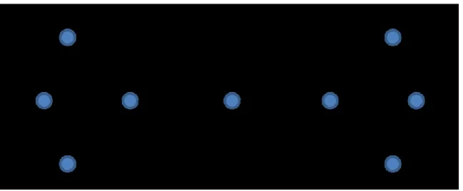
For instance, in the simple graph illustrated in Fig. 2 the values of node displacement reflect the influences of all nodes on a particular one to be analysed. In this example the node

displacements are:



_x

₁





_x

₂





_x

₃





_x

₇





_x

₈





_x

₉



₁

_.

₁₆₅

_,



_x

₄





_x

₆



₀

_.

₇₆₂

and

685

.

0

5





x

, for the nodes with labels given in Fig. 2. This means that the nodes of degree

one are very much affected by the external conditions, which means that they are highly vulnerable. It is easy to realise that these nodes are completely isolated by removing nodes 4 or 6. In addition the removal of node 5 leaves nodes of degree one in an isolated cluster

containing four nodes.

The second most vulnerable nodes according to the displacement are nodes 4 and 6.

They are not affected by the removal of nodes of degree 1 but they are left into an isolated cluster of four nodes when node 5 is removed. Finally, node 5 is the least vulnerable one. It is not affected by the removal of nodes of degree one and when nodes 4 or 6 are removed it still

remains in the largest component of the graph, which is formed by five nodes.

Obviously, the degree fails in ranking the vulnerability of these nodes as it identifies

nodes 4 and 6 as the least vulnerable ones. In addition, betweenness centrality also fails in identifying the least vulnerable node in this graph. The betweenness of nodes 1, 4 and 6 are 0, 18 and 16, respectively, which also identifies node 4 as the least vulnerable one.

Insert Fig. 2 about here.

An explanation of why the displacement is a good measurement of the node

vulnerability can be given in terms of the Laplacian spectrum. We recall that we have ordered

12 3

2







. Then because the eigenvalues of the Laplacian appear in the denominator of the node

displacement (12), the term 2

2 2

i

U

has the largest contribution to x_i. The smallest non-trivial

eigenvalue



2 and its corresponding eigenvector are known as the algebraic connectivity and

the Fiedler vector of the graph, respectively [19]. The Fiedler vector is very well known in spectral graph partitioning [20]. Accordingly, the nodes of the graph are partitioned into two

sets V₁ and V2 as follows: V1



i|Ui20



, V2



i|Ui20



. That is, a node belongs

“strongly” to a partition if it has a large positive or a large negative value of the

corresponding entry of the Fiedler vector, whereas a node with U_i2 close to zero does not belong strongly to either of the two partitions. Consequently, the latter nodes can be considered as “separators” among the partitions. Then, if we remove such separators we in

general isolate the two partitions found by the positive and negative components of the Fiedler vector.

For instance, in the previous example, we have



U

₅₂



0

,



U_{4 2}0.086 _and



U_{1 2} 0.138_.

Of course, the equivalent nodes at the other side of the graph have the same values of the

Fiedler vector but with negative signs. As a first approach we can consider a partition of the graph in which the nodes 1, 2, 3 and 4 form a cluster and the nodes 6, 7, 8 and 9 form another. Then, it is clear that the node 5 is a separator of the two partitions. This means that removing

this separator will isolate the two clusters. In the second approach we can consider that a cluster is formed by nodes 1, 2 and 3, while the other by nodes 7, 8, 9. In this case, the nodes

4, 5 and 6 are separators. As can be seen the node 5 appears as a separator in the two possible partitions and the nodes 4 and 6 in only one of them, which introduces the ranking in vulnerabilities given by the node displacement.

13 graph into isolated components. It is known that



₂





 

_G

, where



 

G

represents the node connectivity, which is the minimum number of nodes that must be removed in order to

disconnect the graph. Then, the two main contributions to the displacement guarantee that the

smallest value of xi is obtained for the nodes contributing more to separate the network into

disconnected parts.

The obvious question at this point is why to use x_i instead of the Fiedler vector as a measure of node vulnerability. First, it has been previously proved that the use of as many

eigenvectors as practically possible should be preferred for partitioning purposes. While the Fiedler vector gives a bipartition of the network the other eigenvectors give partitions into

larger number of clusters, which helps to identify the “separators” in a more appropriate way.

In the second place, the Fiedler vector may be degenerate. That is, the assumption



₂

_



₃ is

not always true, e.g., in square grids and complete graphs. In this case it has been observed

that there are great problems with the convergence of algorithms used for partitioning purposes. Finally, the use of the physically appealing concept of node vibrations permits us also to compare nodes in different networks on the basis of the penalization imposed by the

eigenvalues in the expression for x_i.

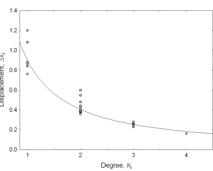
A desired property for a measure of node vulnerability in complex networks is that it accounts in some way for the empirical observation that low-degree nodes are more

vulnerable than the high-degree ones. In Fig. 3 we illustrate the relation between the displacement and the degree for all connected graphs having 5 nodes. It can be seen that the

node displacement correlates with the node degree as _{xi ~ki} with some power





₁

_.

₁₅₅

, which agrees with the intuition that low-degree nodes are more vulnerable than high-degree

14 nodes with the same degree a large variability in their displacements is observed, which adds

an extra value to the use of x_i instead of the node degrees as a measure of node vulnerability.

Insert Fig. 3 about here.

5. Node displacement and information centrality

In the present and next sections we will find exact relations between the node

displacement and other measures. A measure of centrality of a node in a network was introduced by Stephenson and Zelen [18] and is known as information centrality (IC). It is based on the information that can be transmitted between any two points in a connected

network. If A is the adjacency matrix of a network, D a diagonal matrix of the degree of each node and J a matrix with all its elements equal to one, then IC is defined by inverting the

matrix BDAJ as

_C

_

 

_

_B

1

i j

c

, from which the information matrix is obtained as

follows:



_{ 2}



1

 _{ii jj ij}

ij c c c

I (15)

The information centrality of the species i is then defined by using the harmonic average:

 

1

1

1 

    

  





j i j n i I C

I (16)

Stephenson and Zelen [18] proposed to define Iii as infinite for computational purposes,

which makes 1 0

i i

I .

It is straightforward to realise that BLJ. The following theoretic result guarantees

the existence of _CB1

for connected networks.

Lemma 1: If G is a connected network, then the inverse of B has the same eigenvectors as

15



B1_L_ 1

n2J. (17)

where as before L is the Moore-Penrose generalised inverse of L. Proof: Let



k1. Then,

  k k k k k

k U U U U

U  LJ L J 

B _{, (18)}

because JU_k ₀. Now, let



k1_{. Then,} JU1 n U1 due to the fact that ₁ 1 1



n

U  and

because



₁0 and



LU₁ 0 r , we have



B

U

₁



 

L



J

U

₁



L

U

₁



J

U

₁



nU

₁, (19) which means that n is the eigenvalue of B corresponding to



U₁.

It is known that _{LL LL I J} n 1      _,  

LJJ LLJJ L0 and J2nJ_{. Then, we have}

 

LJ

  L _ 1 n2 J  

    I

1

nJ nJ

n2 I, (20)

which proves that



L_ 1

n2J is the inverse of B.

Then, we have the following new result concerning the information centrality.

Theorem 2: Let x_i be the node displacement and



x

 

2

the average displacement over all

nodes in the network. Then, the information centrality of node



i is given by

 

   



2 2



1 x x k i I C

i  

 



. (21)

Proof: Let us write the information centrality as follows

 

_ 



2



_1

n R T c i

I C i i , (22)

where



  n j jj c T 1

and



  n j ij c R 1 . Then,  

c_i _i

 

B1

i iL

_ 1

n2J  

    _i _i

 

L i i

1

n2k

 

xi

2 1

16

 

T c_{j j}

j1

n



T r B1_{T r L}_ 1

n2J  

    T r L

1

n



k

 

xi

2

i1

n



1

n, (24)



R c_{i j}

j1

n





 

B1

i j j1

n



1

n, (25)

because

 

T r J n _and

 

 

₀

1 1  





    n i i j n j

i j L

L . Then, we have

 

 

 

   



2 2



1 1 2 2 2 1 2 1 1 x x k n n n x k n x k i I C i n i i i                               



 

 . (26)

6. Electrical networks analogy

Let us consider a connected network which has associated with an electrical network in such a way that each link of the network is replaced by a resistor of electrical resistance equal to

one Ohm. When the poles of a battery are connected to any pair of nodes i and j in the

network the resulting resistance _ij between them is given by the Kirchhoff and Ohm laws.

Such resistance is known to be a distance function [21] and called the resistance distance. It was introduced in a seminal paper by Klein and Randić a few years ago [21] and has been intensively studied in mathematical chemistry [21-25]. The standard method of computing the

resistance distance for a pair of nodes in a network is by using the Moore-Penrose generalised

inverse of the graph Laplacian L, which is given by [21, 22]

       

ii jj ij ji ij     _{  } 

 L L L L , (27)

for i j. The resistance matrix Ω is the matrix whose non-diagonal entries are _ij and

0





_{i i} [21]. It is easy from Eqs. (12) and (14) to see

 

 



2 2







2

j i i j j i j i

ij  k x  x  x x  x x  k x x

   . (28)

The right-hand side of Eq. (28) should be small when the nodes



i and



j vibrate in the same

17 particularly on the mode corresponding to



₂, on which we discussed in Sec. 4, two nodes in the same partition according to the Fiedler vector vibrate in the same direction and ones in different partitions vibrate in the opposite directions. Then, Eq. (28) dictates that two nodes

that are close in terms of the resistance distance tend to be in the same partition and vibrate in the same direction whereas ones that are far tend to be in different partitions and vibrate in the opposite directions, which fits our intuition well.

The resistance matrix



 is the basis of a topological index for a network that was

introduced first for studying molecular graphs. This index is known as the Kirchhoff index

Kf and is defined as





 

j i

i j

Kf [21-25]. It is known that Kf can be expressed in terms of

the Laplacian eigenvalues as follows [22],





 



1 Tr L

2

n n

Kf n

j j

, (29)

which means that we can express the Kirchhoff index using the node displacements as

 

_x 2 _n2 _k

 

_x 2. k

n

K f n

i i

i  

 







 (30)

This in turn gives the information centrality [18] in the form

 

 

 ₂ 1

  

 _



n Kf i

I C L _{i i} , (31)

where

 

i i k

 

xi 2

 _

L is interpreted here as the contribution of the node to the effective

resistance of every link attached to it. In the case of networks having no cycles, i.e., trees, it is known that the Kirchhoff index and the sum of shortest path lengths between all pairs of

nodes in the graph coincide [21].

Let 





j i j i

R be the sum of the resistance distances from node i to all other nodes in

18

   



_ 2 _{ } 2



_

 

1

n k x x nIC i

Ri  i . (32)

That is, the information centrality measure of a node is inversely proportional to the sum of

the resistance distances from the corresponding node to all other nodes in the network.

7. Application to a social network

The first conclusion from the previous analysis is that for a given network the node

displacement and the information centrality contain exactly the same topological information about the corresponding node, i.e., they are linearly related as

 



   

2 2



/

1 ICi 



k xi  x . (33)

Despite the relationship between the information centrality and the node displacement, there is a fundamental difference between them. The information centrality can be seen as a

composite index containing local information about a node as well as global topological information about the network, whereas with the node displacement we can separate it into

the local information as



x_i

 

2

and the global one as



x

 

2

. This difference is very relevant

when comparing nodes in different networks.

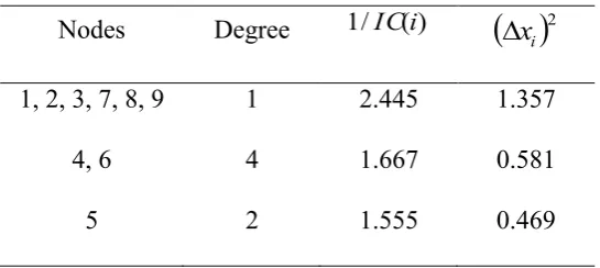
Let us first see the difference using the simple example in Fig. 2. We listed the

breakdown of



1/IC(i) into



x_i

 

2

and



x

 

2

. In terms of the information centrality, the

vulnerability of the nodes 1 and 5 differs only by factor 1.6. In terms of the square node displacement, however, they differ by factor ~3. Moreover, we can claim the following. For

the node 1, we see



xi

 

2

 

 

x 2, which suggests that the vulnerability of the node 1 comes

mainly from its own weak position. For the node 5, on the other hand, we see



xi

 

2

 

 

x 2,

which suggests that the vulnerability of the node 5 comes mainly from the weakness of the entire network, not from its own weakness. This observation suggests that the node

19

Insert Tab. 1 about here.

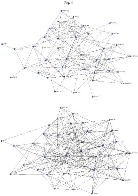
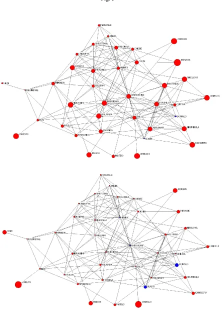
For a more realistic illustration we are going to use the data obtained by Kapferer about the social ties among tailor shops in Zambia [26]. Hereafter we use the parameter value of



k1, for which the vibrational energy is comparable to the thermal energy. The network is

formed by 39 individuals who were observed during a period of ten months for their friendship and socio-emotional relationships. The data consists of two networks of social

interactions recorded at two different times [26, 27]. After the first data was collected an abortive strike was reported [26]. Then, after seven months the second data was collected and

a successful strike took place after it. In Fig. 4 we illustrate the social interactions between the 39 people in the tailor shop at the two different times.

Insert Fig. 4 about here.

We have proved analytically that the information centrality and the node displacement are directly related to each other for the nodes of a network. Then, we focus here on the

differences between the two indices when we compare the same nodes in two different versions of the same network. For the purpose, we are going to use the change in the

information centrality after seven months in the tailor shop IC

 

i IC₂

 

i IC₁

 

i , where

 

i

IC_t is the information centrality of node i at time step t. In a similar way we define xi

as the difference in the node displacement at the two times in which the network was

analysed. In Fig. 5 we represent the differences in



IC



i

and x_i for all nodes in the tailor

shop. For the sake of comparison, the values of

 

2

x

 for these two versions of the tailor shop

network are 0.242 and 0.129, respectively.

Insert Fig. 5 about here.

This example clearly illustrates the differences between the information centrality and

the node displacement in characterization of nodes. According to I C

 

i _{the individuals that}

20 Chipata > Kamwefu > Ibrahim > Mukubwa > Nkoloya > Enoch. However, the ranking

according to the node displacements is: Zakeyo > Chipalo > Adrian > Sign > Enoch > Donal > Meshak > Seans > Kamwefu > Chipata. Meshak, who is ranked as number one according to

 

i I C

 _{, is the actor displaying the largest change in the degree among all the actors. It}

changes its degree from 4 to 18 in the two versions of the tailor shop. However, Zakeyo and

Chipalo, who are ranked by xi as the ones having the largest change in the node

displacement have changed their degree from 1 to 7 in the two versions of the tailor shop

network.

According to Eq. (33), the increase in the information centrality of a node can mean either the decrease in the local node displacement or the decrease in the global (average) node

displacement (or both). Comparing the two panels in Fig. 5, we realise that the increase of the information centrality is, for most nodes, due to the decrease of the average node

displacement, not due to the local one. Many nodes had many links in the first place and were not very vulnerable. Their information centrality increased after seven month mainly because

the number of links generally increased in the entire network and hence



x

 

2

decreased,

whereas their own node displacement scarcely decreased, that is, their own local vulnerability scarcely changed. For some nodes such as Zakeyo and Chipalo, however, their own

vulnerability improved greatly after seven months because their own degrees increased dramatically. This demonstrates clearly that the node displacement has a better resolution of

the situation than the information centrality.

In general, the change in the information centrality is very much correlated with the

change in the degree centrality DC

 

i . For instance, the correlation coefficient between

 

i

I C

 _and

_

_DC



_i

_{is 0.87 for the nodes in the network analysed here. However,} x_i

21 very well these differences is provided by the ranking of Sign, who is ranked as the fourth

largest change in xi among all actors in the tailor shop. He is ranked as number 36 out of

39 according to the change in the information centrality and between 29 and 32 according to the change of the degree centrality, which is only 1. Sign was in a very vulnerable position in

the initial network as he was connected to only one actor. After seven months he displayed a less vulnerable position in the network as he appears connected to two other actors. In the cases of Zakeyo and Chipalo this change has been more dramatic as they increased their

degree from 1 to 7 in the two versions of the network and they appear as the ones having the

largest changes in xi.

8. Summary

In the present paper we proposed the node displacement as a measure of vulnerability of each node in a network. We defined the node displacement as the amplitude of vibration caused by

thermal fluctuation of a heat bath. This simulates the situation where the network in question is under a level of external stress. We proved exact relations among the node displacement,

the information centrality and the Kirchhoff index. The relation between the first two suggested that the node displacement has a better resolution of vulnerability than the information centrality; the latter is the sum of the local node displacement and the averaged

22

References

[1] L.C. Freeman, Sociometry 40 (1977) 35. [2] S.P. Borgatti, Social Networks 27 (2005) 55.

[3] S. Wasserman, K. Faust, Social Network Analysis, Cambridge University Press,

Cambridge, 1994.

[4] H. Jeong, S.P. Mason, A.-L. Barabási, Z.N. Oltvai, Nature 411 (2001) 41.

[5] E. Estrada, Proteomics 6 (2006) 35.

[6] G. del Rio, D. Koschutzki, G. Coello, BMC Syst. Biol. 3 (2009) 102. [7] F. Jordan, Phil. Trans. Royal Soc. B, Biol. Sci. 364 (2009) 1733.

[8] E. Estrada, Ö. Bodin, Ecol. Appl. 18 (2008) 1810.

[9] M. Barthelemy, A. Barrat, A. Vespignani, Adv. Compl. Syst. 10 (2007) 5.

[10] J.H. Choi, G.A. Barnett, B.S. Chou, Global Networks 6 (2006) 81. [11] L.C. Freeman, J. Soc. Struct. 9 (2008) 1.

[12] P. Holme, B.J. Kin, C.N. Yoon, S.K. Hau, Phys. Rev. E 65 (2002) 056109.

[13] L. Zhao, K. Park, Y.-C. Lai, Phys. Rev. E 70 (2004) 035101.

[14] J. Wang, L. Dong, D.J. Hill, G.H. Zhang, Physica A 387 (2008) 6671.

[15] A. Santiago, R.M. Benito, Physica A 388 (2009) 2234.

[16] G. Chen, Z.Y. Dong, D.J. Hill, G.H. Zhang, Physica A 388 (2009) 4259.

[17] R. Albert, H. Jeong, A.-L. Barabási, Nature 406 (200) 378. [18] K. Stephenson, M. Zelen, Social Networks 11 (1989) 1.

[19] M. Fiedler, Czech. Math. J., 23 (1973) 298.

[20] D.A. Spielman, S.-H. Teng, Lin. Algebra Appl. 421 (2007) 284. [21] D.J. Klein, M. Randić, J. Math. Chem. 12 (1993) 81.

[22] W. Xiao, I. Gutman, Theor. Chem. Acc. 110 (2003) 284.

23 [24] H.Y. Chen, F.J. Zhang, Disc. Appl. Math. 155 (2007) 654.

[25] B. Zhou, N. Trinajstić, J. Math. Chem. 46 (2009) 283.

[26] B. Kapferer, Strategy and transaction in an African factory. Manchester University Press, Manchester, 1972.

[image:24.595.163.436.226.348.2]

24

Table 1

Tab. 1: Inverse of the information centrality and the squared node displacement for the nodes

of the network shown in Fig. 2. These two measures satisfy Eq. (33) with

 

x2 1.086 and



k1.

Nodes Degree 1/IC(i)

 

x_i 2 1, 2, 3, 7, 8, 9 1 2.445 1.357

4, 6 4 1.667 0.581

25

Figure Captions

Fig. 1: A network submerged in a thermal bath. A “gas” at



T_{, a “liquid” at}



T



1

, and a

“solid” at



T



0

.

Fig. 2: A simple network for illustration.

Fig. 3: Correlation between the node degree and the node displacement. The solid curve

indicates the power-law relation



xi ~ki

1.155

, with correlation coefficient 0.958.

Fig. 4: The social network of 39 tailor shops in Zambia at one time (top) and seven months

after that (bottom).

Fig. 5: Temporal changes in the information centrality and the node displacement. Each node

is drawn with a diameter proportional to the absolute value of



_IC

 

_i

_{(top) or}





x

_i

(bottom), respectively. In the upper panel, the red circles indicate the nodes where their information centrality increased (less vulnerability) and the blue ones indicate the nodes

where it decreased (more vulnerability). In the lower panel, the red circles indicate the nodes where the node displacement increased (less vulnerability) and the blue ones indicate the

26

Fig. 1

0

   

T 1

   

0 T

[image:27.595.136.461.121.255.2]

[image:28.595.83.519.112.461.2]

[image:29.595.75.522.71.707.2]

[image:30.595.81.526.82.711.2]