City, University of London Institutional Repository
Citation
: Dash, J., Lankester, T., Hubbard, S. & Curran, P. J. (2008). Signal-to-noise ratio
for MTCI and NDVI time series data. Paper presented at the 2nd MERIS/(A)ATSR User
Workshop, 22 - 26 September 2008, Rome.
This is the published version of the paper.
This version of the publication may differ from the final published
version.
Permanent repository link:
http://openaccess.city.ac.uk/12837/
Link to published version
:
Copyright and reuse:
City Research Online aims to make research
outputs of City, University of London available to a wider audience.
Copyright and Moral Rights remain with the author(s) and/or copyright
holders. URLs from City Research Online may be freely distributed and
linked to.
City Research Online:
http://openaccess.city.ac.uk/
publications@city.ac.uk
SIGNAL-TO-NOISE RATIO FOR MTCI AND NDVI TIME SERIES DATA
J. Dash
(1), T. Lankester
(2), S. Hubbard
(2), and P. J. Curran
(3)(1) School of Geography, University of Southampton, Southampton SO17 1BJ, UK, jadu@soton.ac.uk
(2)Infoterra Ltd., Europa House, The Crescent, Farnborough GU14 0NL, UK,thomas.lankester@infoterra-global.com
(2)Office of Vice-Chancellor, Bournemouth University, Talbot Campus, Fern Barrow, Poole BH12 5BB, UK
pcurran@bournemouth.ac.uk
ABSTRACT
The Phenology of vegetation varies with climate and variability in phenology is a powerful measure of climate change. Remotely-sensed data can be used to produce phenology curves that capture ‘green-up’, maturity and senescence from local to global scales. These curves are usually produced with Normalised Difference Vegetation Index (NDVI) data but are notoriously noisy. The MERIS Terrestrial Chlorophyll Index (MTCI) is related to the chlorophyll content, does not suffer from some of the limitations of NDVI (e.g., saturation at high biomass) and should, it was hypothesised, produce a less noisy phenological curve. Two methods were used to determine the phenological curve (signal) and Variability in the curve (noise); iterative polynomial fitting and discrete Fourier transformation.
The signal-to-noise ratio (SNR) for MTCI curves was significantly higher than for the NDVI curves and this difference was largest for high green biomass areas. This was probably the result of the compositing techniques typically used for MTCI data. However, the two methods of SNR calculation produced different results for the NDVI but not the MTCI, thus suggesting that there was bias in the less noisy NDVI curve.
1. INTRODUCTION
Climate influences vegetation growth and more specifically increased temperature and level of atmospheric carbon dioxide increases vegetation productivity, carbon sequestration and modifies ecosystem function [1, 2]. The estimation, in space and time, of vegetation phenological variables such as: time of onset of ‘greenness’, time of end of ‘greenness’, duration of the growing season, rate of ‘green up’ and rate of senescence can provide the information needed to understand better the effect of climate change on vegetation. Such phenological variables can be derived from ground or remotely sensed data. Ground-derived phenological variables
provide species-specific information with high
temporal resolution but lack a spatial component [3]. By contrast, temporally frequent remotely sensed data provide a unique opportunity to estimate phenological variables at a range of scales from local to global. The normalised difference vegetation index (NDVI), ratio
of reflected solar radiation in red and near-infrared wavebands, is used widely to estimate phenological variables [4]. Many studies have used an NDVI time series calculated using the Advanced Very High Resolution Radiometer (AVHRR) sensor data to first, derive phenological variables and then use this information to quantify ecosystem response to climate change over continents and decades [5, 6, 7, 8]. These studies have been made possible by the high correlation between NDVI and the amount of green vegetation biomass [6]. However, most of the studies suffered from unexplained variations in a smooth growth curve, as a result of image miss-alignment, sensor miss-calibration [9] and changing atmospheric conditions [10], for example, temporal variation in the presence of cloud, water, snow, or shadow [11, 12]. As a result, it has proved difficult to derive reliable routine phenological variables from raw NDVI time series data [5]. Smoothing methods have been developed to suppress this sensor and environmental ‘noise’ in the phenological signal. Examples include median smoothing [5], discrete Fourier transforms [13], moving averages [14] and Savitzky-Golay filters [15].
Furthermore, the NDVI which varies with both the amount of green vegetation biomass and the concentration of chlorophyll [11, 16, 17] saturates at high levels of both. Satellite sensor systems such as EOS and Envisat and in the future, Sentinel 3, could go some way to addressing this constraint. An operational ESA Envisat product, the MERIS Terrestrial Chlorophyll Index (MTCI), is related directly to canopy chlorophyll content [18], which is, in turn, a function of chlorophyll concentration and leaf area index [19]. MTCI has limited sensitivity to atmospheric effects and also soil background and view angle [20] and with the availability of near real time weekly and global MTCI composites [21] enables researchers to derive accurate phenological variables accurately. However, given the previous experience with the NDVI, it is important to estimate the amount of sensor and environmental noise present in the MTCI time series before using it to derive these phenological variables.
The aim of this study was to estimate and compare the Signal-to-Noise Ratio (SNR) in both NDVI and MTCI time series for different land cover types as a prelude to the use of the MTCI for regional to global scale phenological investigations.
_________________________________________
2. DATA METHODOLOGY
Although most remote sensing studies of vegetation phenology have used NDVI calculated using AVHRR data, the NDVI derived from the spatially, spectrally
and radiometrically more appropriate SPOT
VEGETATION sensor are the most accurate available in routinely available datasets [22]. For this study, a time series of SPOT VEGETATION NDVI composite (S10) products was obtained from the VGT4Africa project [23].
The S10 NDVI product is derived from 10 day periods or dekads of NDVI data [24], mapped onto a 1km latitude-longitude grid using a Maximum Value Composite (MVC) algorithm. For each pixel in the grid, the MVC algorithm selects the most probable NDVI value [23] during the dekad period. If two, or more, NDVI values have the same probability then the maximum value is used.
MTCI data was composited from standard ESA Level
2 (geophysical) products using an identical
compositing period (dekads) and map grid (latitude-longitude, 112 pixels per degree) as those used for the S10 NDVI product. The MTCI value compositing algorithm differed, however, from the VGT4Africa MVC algorithm in that all valid MTCI values were combined using an arithmetic mean. As a result, the S10 NDVI data have already undergone, what is in effect, a noise reduction procedure whereas MTCI composite data have not.
Eight dominant land cover types were selected using the University of Maryland (UMD) thirteen class, 1 km spatial resolution land cover map. The UMD land cover map had been prepared using AVHRR data acquired between 1991-1994 [25]. The NDVI composite, MTCI composite and land cover map were co-registered and for each land cover type pixels were selected from across Africa.
Two techniques were used to estimate the ‘signal’ (the smooth time series curve) and the ‘noise’ (variability around the time series curve): (i) Iterative polynomial fitting and (ii) discrete Fourier transformation.
2.1. Iterative polynomial fitting
The iterative polynomial algorithm divides the time
series T, into a set of n, 21 dekad long, time series (Tn)
with an overlap of 6 dekad between each time series.
For each n a 5th order polynomial (Pn) was fitted to
each series (Tn)
For each overlapping period the data were averaged.
The resultant smooth time series is Sn is defined as :
Sn =Max (Tn, Pn ) (1)
This process was repeated 6 times and the 5th degree
polynomial ensures that the curve cannot have more than 4 extrema (2 minima and 2 maxima) during the 21 dekad time period.
2.2. Discrete Fourier transformation
The discrete Fourier transformation (DFT) decomposes any complex waveform into a series of sinusoids of different frequency. Individual sinusoids and their frequencies can be amalgamated in to a complex waveform for which noise has been removed. The DFT is given by:
∑
−=
−
=
10
/ 2 )
(
(
)
*
1
N xT ux u
f
x
e
N
F
π (2)Where f(x) is the xth value in the time series, u is the
number of Fourier components, x is the dekad number,
T is the length of time period cover (number of dekad), and here T is equal to N.
The above equation consists of two parts: cosine (real) part and sine (imaginary part), where the cosine part is:
)
2
cos(
*
)
(
(
1
10 )
(
∑
−
=
=
Nx u
C
T
ux
x
f
N
F
π
(3)And the sine part is
)
2
sin(
*
)
(
(
1
10 )
(
∑
−
=
=
Nx u
S
T
ux
x
f
N
F
π
Using the above equation the Fourier magnitude (Fm)
can be calculated as
2 ) ( 2
) ( )
(u Cu S u
m
F
F
F
=
+
And the phase (Fp) can be calculated as
=
) (
) ( )
(
tan
2
u S
u C u
p
F
F
a
F
The first two harmonics of the Fourier transformation usually account for 50-90% of the variability in a data set; in this case variability in the vegetation index time series [13, 26]. Inverse Fourier transformation using the first two harmonics alone has been used successfully by others to recreate an NDVI ‘profile’ for the identification of crop types [26], agro-ecological zones [27] and broad land cover types [28]. It has been suggested that phenologically related information exists within the fist five harmonics with higher order harmonics dominated by noise [29].
2.3. Estimating Signal-to-Noise ratio (SNR)
We assumed that the smooth curves obtained by iterative polynomial fitting and inverse Fourier transformation were ‘signal’ and the difference between this smooth curve and the raw data were ‘noise’. The SNR can be estimated as:
Noise signal Signal
StDev
Min
Max
SNR
=
−
(4)0 0.25 0.5 0.75 1
0 5 10 15 20 25 30 35 40
Time (Layer number)
N D V I v a lu e -0.1 0 0.1 0.2
0 5 10 15 20 25 30 35 40
Time (Layer number)
M T C I n o rm a li s e d n o is e -0.1 0 0.1 0.2
0 5 10 15 20 25 30 35 40
Time (Layer number)
N D V I n o rm a li s e d n o is e
3. RESULTS AND DISCUSSION
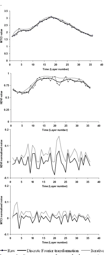
For a broadleaved forest pixel a comparison between the smoothed curve derived using both iterative polynomial fitting and discrete Fourier transformation and raw data for the MTCI and NDVI is shown in Fig. 1. 0 0.5 1 1.5 2 2.5 3 3.5
0 5 10 15 20 25 30 35 40
Time (Layer number)
M T C I v a lu e
Figure 1. Comparison of smoothed curve (signal) and raw data using discrete Fourier transformation & iterative polynomial fitting for MTCI & NDVI for a deciduous broadleaved pixel and the normalised noise.
The iterative polynomial curve was fitted along the highest values, as NDVI values were, in general, lowered by sensor and environmental noise. The discrete Fourier transformation makes no such assumptions and fitted the curve through the middle of the time series points.
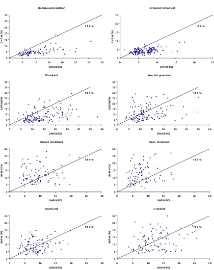
The MTCI and NDVI SNR for each land cover type were compared using scatter plots (Fig. 2 and 3) and as would be expected, there was no correlation between the two. However, the MTCI SNR was high for the high green biomass classes (deciduous broadleaf, evergreen broadleaf, woodland, wooded grassland) and the NDVI SNR was slightly higher for the intermediate green biomass class (shrubland). Moreover, the MTCI SNR was more than twice that of NDVI SNR for deciduous broadleaf, evergreen broadleaf and woodland (table 1). As discussed above iterative polynomial fitting produced a slightly lower
NDVI SNR than that of discrete Fourier
transformation. Deciduous broadleaf 0 5 10 15 20 25 30 35
0 5 10 15 20 25 30 35 SNR MTCI S N R N D V I 1:1 line Evergreen broadleaf 0 5 10 15 20 25
0 5 10 15 20 25 SNR MTCI S N R N D V I 1:1 line Woodland 0 5 10 15 20 25 30 35 40
0 5 10 15 20 25 30 35 40 SNR MTCI S N R N D V I 1:1 line Wooded grassland 0 5 10 15 20 25 30
0 5 10 15 20 25 30 SNR MTCI S N R N D V I 1:1 line Closed shrubland 0 5 10 15 20 25 30
0 5 10 15 20 25 30 SNR MTCI S N R N D V I 1:1 line Open shrubland 0 5 10 15 20 25 30
0 5 10 15 20 25 30 SNR MTCI S N R N D V I 1:1 line Grassland 0 5 10 15 20 25 30
0 5 10 15 20 25 30 SNR MTCI S N R N D V I 1:1 line Cropland 0 5 10 15 20 25 30
0 5 10 15 20 25 30 SNR MTCI S N R N D V I 1:1 line
Figure 2. Relationship between MTCI SNR and NDVI SNR for eight land cover classes using iterative polynomial fitting.
Table1. Mean and standard deviation (SD) of MTCI SNR and NDVI SNR for eight land cover classes estimated using the discrete Fourier transformation(DFT) and iterative polynomial fitting(IPF).
Mean SNR using IPF
Mean SNR using DFT Land cover class
No of
points MTCI NDVI MTCI NDVI
Deciduous broadleaf 82 11.15 4.04 10.82 5.26
Evergreen broadleaf 139 7.09 2.90 6.70 4.17
Woodland 138 14.45 7.44 14.71 8.64
Wooded grassland 121 12.31 10.19 12.91 11.36
Closed shrubland 92 9.25 11.05 9.94 12.74
Open shrubland 99 9.30 10.43 8.08 12.20
Grassland 101 9.05 8.03 8.79 9.27
[image:4.595.61.244.139.588.2] [image:4.595.317.536.149.501.2]Deciduous broadleaf 0 5 10 15 20 25 30 35
0 5 10 15 20 25 30 35 SNR MTCI S N R N D V I 1:1 line Evergreen broadleaf 0 5 10 15 20 25
0 5 10 15 20 25 SNR MTCI S N R N D V I 1:1 line Woodland 0 5 10 15 20 25 30 35 40
0 5 10 15 20 25 30 35 40 SNR MTCI S N R N D V I 1:1 line Wooded grassland 0 5 10 15 20 25 30 35 40
0 5 10 15 20 25 30 35 40 SNR MTCI S N R N D V I 1:1 line Closed shrubland 0 5 10 15 20 25 30
0 5 10 15 20 25 30 SNR MTCI S N R N D V I 1:1 line Open shrubland 0 5 10 15 20 25 30
0 5 10 15 20 25 30 SNR MTCI S N R N D V I 1:1 line Grassland 0 5 10 15 20 25 30
0 5 10 15 20 25 30 SNR MTCI S N R N D V I 1:1 line Cropland 0 5 10 15 20 25 30
[image:5.595.59.277.67.342.2]0 5 10 15 20 25 30 SNR MTCI S N R N D V I 1:1 line
Figure 3. Relationship between MTCI SNR and NDVI SNR for eight land cover classes using discrete Fourier transformation.
The Mann-Whitney U test was used to determine (i) if there was a significant difference between SNR produced using the two methods and (ii) if variation in SNR in MTCI and NDVI was significant. The Mann-Whitney U-Test examines whether the differences between two sets of sample data are significant or whether these differences could have occurred by chance.
For NDVI time series and for most land cover classes either there was a significant (p<0.001) or marginally significant (p<0.05) difference between the SNR produced using the two methods (table 2). By contrast, for MTCI time series and for most land cover classes (except cropland) there was no significant difference between the SNR produced using the two methods (table 2). This was because the iterative polynomial was fitted to high values of NDVI and the discrete Fourier transformation produced a curve that passed through the middle of the time series points. Therefore, when there was a data ‘drop out’ in the NDVI time series the difference between raw and processed data was higher when iterative polynomial fitting than when using discrete Fourier transformation; resulting in a higher noise and lower SNR for the former method. As there was no significant difference between the SNR produced by both methods in the MTCI time series curve, it can be inferred that there is no bias in the MTCI noise. It suggested that MTCI noise is more randomly distributed around the signal and so does not results in the data ‘drop outs’ seen in NDVI data.
SNR for NDVI SNR for MTCI
Land cover class
Z p Z p
Deciduous broadleaf -3.516 <0.001 -0.326 0.745
Evergreen broadleaf -6.877 <0.001 -0.222 0.824
Woodland -2.213 0.027 -0.829 0.407
Wooded grassland -1.134 0.257 -0.310 0.756
Closed shrubland -2.127 0.033 -1.005 0.315
Open shrubland -1.822 0.069 -1.503 0.133
Grassland -2.053 0.040 -0.393 0.694
Cropland -2.185 0.029 -2.348 0.019
Table 2. Mann Whitney Z and p values for MTCI SNR and NDVI SNR between SNR estimated using the discrete Fourier transformation and iterative polynomial fitting. SNR using discrete Fourier transformation SNR using iterative polynomial fitting Land cover class
Z p Z p
Deciduous broadleaf -8.728 <0.001 -7.715 <0.001
Evergreen broadleaf -12.191 <0.001 -8.698 <0.001
Woodland -9.078 <0.001 -8.031 <0.001
Wooded grassland -3.219 0.0013 -2.875 0.0040
Closed shrubland -2.274 0.0230 -2.666 0.0077
Open shrubland -1.558 0.1192 -4.829 <0.001
Grassland -1.842 0.0655 -0.629 0.5292
Cropland -1.169 0.2425 -0.675 0.4991
Table 3. Mann Whitney Z and p values for SNR estimated using the discrete Fourier transformation and iterative polynomial fitting between the MTCI SNR and NDVI SNR.
[image:5.595.312.526.81.217.2]noise within the compositing period then the MTCI SNR would be even higher.
4. CONCLUSION
The SNR for NDVI and MTCI time series were determined for eight land cover types using iterative polynomial fitting and discrete Fourier transformation. A maximum value compositing method was used to produce NDVI composites; whereas an arithmetic mean was used to produce MTCI composites. It can be conluded from this study that:
(i) The MTCI SNR was significantly higher than
NDVI SNR for areas of high green biomass. However, the MTCI SNR could have been increased by adopting a better composting method which could remove outliers that contribute to noise.
(ii) There was a statistically significant difference
between NDVI SNR estimated using the two methods which suggested a bias in NDVI time series as a result of sensor and environmental noise.
(iii)There was no significant difference between MTCI
SNR estimated using the two methods which suggested MTCI was less affected by sensor and environmental noise.
Other criteria, such as phenological variable
determination, are subject to further comparison. The future work should focus on:(i) alternate filtering for MTCI compositing e.g. median instead of mean to reduce the effect of outlier values and (ii) comparison in areas of know NDVI value ‘dropouts’ (e.g., along the Gulf of Guinea in Africa) to see if MTCI is degraded to the same extent.
5. ACKNOWLEDGEMENT
The authors acknowledge the NERC Earth Observation Data Centre for MTCI composites; VGT4Africa project, SPOT Vegetation programme and CNES for NDVI composite data and Mr Jonathan Rumsey for help in data processing.
6. REFERENCES
1. Rosenzweig, C. & M. L. Parry. (1994). Potential impact of climate-change on world food-supply,
Nature, vol. 367, no. 6459, pp. 133-138.
2. Diaz, S., Grime, J. P., Harris, J. & Mcpherson, E. (1993). Evidence of a feedback mechanism limiting plant-response to elevated
carbon-dioxide, Nature, vol. 364, no. 6438, pp.
616-617.
3. Studer, S., Stockli, R., Appenzeller, C. & Vidale, P. L. (2007). A comparative study of satellite and
ground-based phenology, International Journal
of Biometeorology, vol. 51, no. 5, pp. 405-414. 4. Rouse, J. W., Haas, R. H., Schell, J. A. & Deering,
D.W. (1974). Monitoring vegetation systems in
the Great Plains with ERT, In Proceedings,
Third Earth Resources Technology Satellite-1 Symposium, Greenbelt: NASA SP-351, pp. 309-317.
5. Reed, B. C., Brown, J. F., Vanderzee, D., Loveland, T. R., Merchant, J. W. & Ohlen, D. O. (1994).
Measuring phenological variability from
satellite imagery, Journal of Vegetation Science,
vol. 5, no. 5, pp. 703-714.
6. Myneni, R. B., Keeling, C. D., Tucker, C. J., Asrar, G. & Nemani, R. R. (1997). Increased plant growth in the northern high latitudes from 1981
to 1991, Nature, vol. 386, no. 6626, pp.
698-702.
7. Zhou, L. M., Tucker, C. J., Kaufmann, R. K., Slayback, D., Shabanov, N. V. & Myneni, R. B. (2001). Variations in northern vegetation activity inferred from satellite data of vegetation
index during 1981 to 1999, Journal of
Geophysical Research-Atmospheres, vol. 106, no. D17, pp. 20069-20083.
8. White, M. A., Hoffman ,F., Hargrove, W. &. Nemani, R. (2005). A global framework for monitoring phenological responses to climate
change, Geophysical Research Letters, vol. 32,
no. 4, doi:10.1029/2004GL021961.
9. Vermote, E. & Kaufman, Y. J. (1995). Absolute calibration of AVHRR visible and near-infrared channels using ocean and cloud views,
International Journal of Remote Sensing, vol. 16, no. 13, pp. 2317-2340.
10. Tanre, D., Holben, B. N. & Kaufman, Y. J.(1992). Atmospheric correction algorithm for NOAA-AVHRR products - Theory and application,
IEEE Transactions on Geoscience and Remote Sensing, vol. 30, no. 2, pp. 231-248.
11. Huete, A., Didan, K., Miura, T., Rodriguez, E. P., Gao, X. & Ferreira, L. G. (2002). Overview of the radiometric and biophysical performance of
the MODIS vegetation indices, Remote Sensing
of Environment, vol. 83, no. 1-2, pp. 195-213. 12.Goward, S. N., Markham, B., Dye, D. G., Dulaney,
W. & Yang, J. L. (1991). Normalized Difference Vegetation Index measurements from the Advanced Very High-Resolution Radiometer,
Remote Sensing of Environment, vol. 35, no. 2-3, pp. 257-277.
13. Moody A. & Johnson, D. M. (2001). Land-surface phenologies from AVHRR using the discrete
Fourier transform, Remote Sensing of
Environment, vol. 75, no. 3, pp. 305-323. 14. Tieszen, L. , Reed, B. C., Bliss, N. B., Wylie, B. K.
& Dejong, D. (1997). NDVI, C-3 and C-4 production, and distributions in Great Plains
grassland land cover classes, Ecological
15.Zhang, X. Y., Friedl, M. A., Schaaf, C. B., et al. (2003). Monitoring vegetation phenology using
MODIS, Remote Sensing of Environment, vol.
84, no. 3, pp. 471-475.
16. Gitelson, A. A. & Kaufman, Y. J. (1998).
MODIS NDVI optimization to fit the AVHRR
data series spectral considerations, Remote
Sensing of Environment, vol. 66, no. 3, pp. 343-350.
17. Mutanga O. & Skidmore, A. K. (2004). Narrow band vegetation indices overcome the saturation
problem in biomass estimation, International
Journal of Remote Sensing, vol. 25, no. 19, pp. 3999-4014.
18.ESA (2007). MERIS chlorophyll data proves
positive [online]. Available:
http://www.esa.int/esaLP/SEMADLSMTWE_L Pcampaigns_0.html
19.Dash, J. & Curran, P. J. (2004). The MERIS
Terrestrial Chlorophyll Index, International
Journal of Remote Sensing, vol. 25, no. 23, pp. 5403-5413.
20.Curran, P. J. & Dash, J. (2005). Algorithm
theoretical basis document (ATBD):
Chlorophyll Index-Version 2.2”, European Space Agency, Noordwijk, The Netherlands [online].Available:
envisat.esa.int/instruments/meris/atbd/atbd_2_2 2.pdf .
21. Curran, P. J., Dash, J., Lankester, T. & Hubbard,S. (2007). Global composites of the MERIS
Terrestrial Chlorophyll Index, International
Journal of Remote Sensing, vol. 28, no.18, pp. 3757-3758.
22.Tucker, C. J., Pinzon, J. E., Brown, M. E. et al. (2005). An extended AVHRR 8-km NDVI dataset compatible with MODIS and SPOT
vegetation NDVI data, International Journal of
Remote Sensing, vol. 26, no. 20, pp. 4485-4498. 23. Baret, F., Bartholomé, E., Bicheron, P. et al.
(2006). VGT4Africa User Manual [online]. Available:
http://www.vgt4africa.org/PublicDocuments/VG
T4AFRICA_user_manual.pdf.
24.World Meteorological Organization, “International Meteorological Vocabulary”, 2nd edn. WMO: Geneva, Switzerland. WMO Publication 182, 1992.
25. Hansen, M., DeFries, R., Townshend, J. R. G. & Sohlberg, R. (1994). UMD Global Land Cover Classification, 1 Kilometer, 1.0, Department of Geography, University of Maryland, College Park, Maryland.
26. Jakubauskas, M. E., Peterson, D. L., Kastens, J. H. & Legates, D. R. (2002). Time series remote sensing of landscape-vegetation interactions in
the southern Great Plains, Photogrammetric
Engineering and Remote Sensing, vol. 68, no. 10, pp. 1021-1030.
27. Menenti, M., Azzali, S., Verhoef, W. & Vanswol, R. (1993). Mapping agroecological zones and time-lag in vegetation growth by means of Fourier-analysis of time-series of NDVI images,
Advances in Space Research, vol. 13, no. 5, pp. 233-237.
28. Andres, L., Salas, W. A. & Skole, D. (1994). Fourier-analysis of multitemporal AVHRR data
applied to a land-cover classification,
International Journal of Remote Sensing, vol. 15, no. 5, pp. 1115-1121.
29. Geerken, R., Zaitchik, B. & Evans, J. P. (2005). Classifying rangeland vegetation type and coverage from NDVI time series using Fourier
filtered cycle similarity, International Journal of
Remote Sensing, vol. 26, no. 24, pp. 5535–5554.