Scheduling reentrant jobs on parallel machines with a remote server

City, University of London Institutional Repository

Citation:

This is the unspecified version of the paper.

This version of the publication may differ from the final published

version.

Permanent repository link:

Link to published version:

Copyright and reuse: City Research Online aims to make research

outputs of City, University of London available to a wider audience.

Copyright and Moral Rights remain with the author(s) and/or copyright

holders. URLs from City Research Online may be freely distributed and

linked to.

Faculty of Actuarial

Science

and

Insurance

Statistical Research Paper

No. 30

Scheduling Reentrant Jobs on

Parallel Machines with a Remote

Server

Konstantin Chakhlevitch

Celia Glass

October 2008

Cass Business School

106

Bunhill

Row

London

EC1Y

8TZ

Scheduling reentrant jobs on parallel machines with a

remote server

K. Chakhlevitch

_{and C.A. Glass}

Cass Business School, City University London, 106 Bunhill Row, EC1Y 8TZ, UK

Konstantin.Chakhlevitch.1@city.ac.uk, C.A.Glass@city.ac.uk

Abstract

This paper explores a specific combinatorial problem relating to re-entrant jobs on parallel primary machines, with a remote server machine. A middle operation is required by each job on the server before it returns to its primary processing machine. The problem is inspired by the logistics of a semi-automated micro-biology laboratory. The testing programme in the laboratory corresponds roughly to a hybrid flowshop, whose bottleneck stage is the subject of study. We demonstrate the NP-hard nature of the problem, and provide various structural features. A heuristic is developed and tested on randomly generated benchmark data. Results indicate solutions reliably within 1.5% of optimum. We also provide a greedy 2-approximation algorithm. Test on real-life data from the microbiology laboratory indicate a 20% saving relative to current practice, which is more than can be achieved currently with 3 instead of 2 people staffing the primary machines.

Keywords: scheduling, parallel identical machines, remote server, reentrant jobs

1

Introduction

The scheduling problem considered in this paper arises from the technological process ob-served in a microbiological laboratory. The laboratory performs microbiological testing on samples of processed foods prior to release to retailers. Each food sample undergoes a suite of tests, which is specified in advance. Each test suite consists of a number of micro-biological tests, carried out by scientists with the aid of semi-automated equipment. The samples proceed through a number of consecutive processes, which include weighing, pipet-ting out onto test plates and a period of incubation. According to their test suite, samples require different dilutions, and tests on the samples require different types of media and in-cubation times for bacterial development, among other things. The laboratory is equipped with a fully integrated Laboratory Information Management System (LIMS) which controls individual tests for each sample. Pathogen tests are carried out in a separate laboratory. Thus, all samples in the main laboratory may be processed without risk of contamination. The logistics of testing in the microbiology laboratory may be viewed as a type of hybrid flowshop, with sets of parallel machines, performing similar functions, at various stages. However, one of the stages, namely the pipetting stage, appears as the bottleneck stage in

the whole testing process. The test samples are pipetted onto test plates which must be assembled and labelled ready for the purpose. The test plates are prepared by a dedicated machine, which serves several pipetting stations. The interaction between the single plate labelling machine and the pipetters working in parallel, gives rise to an unusual scheduling problem which is the subject of this paper.

The problem may be formulated in terms of a set of m parallel primary machines,

M1, M2, M3, . . . , Mm (the pipetters) and a single server machine S (the plate labelling machine). Jobs have three operations, the first and last of which are performed by the same pipetter, Mi say, with a middle operation on the server, S. The issue is not one of sequencing operations, as the order of jobs and of each of their operations is predetermined in our context. The challenge is that of assigning jobs to the primary machines. We restrict attention to the case of identical machines. We refer to this as the Initialization-Setup-Processing, ISP, problem. To the best of our knowledge, the ISP problem has not been studied before.

The scenario described above can be modelled using a parallel machines with a common server environment. A range of problems thus classified has been considered in the litera-ture. Complexity results for problems with identical parallel machines with a single server and different objective functions were obtained by Hall et al. [1], Brucker et al. [2] and Kravchenko and Werner [3]. Abdekhodaee and Wirth [4] studied some solvable cases of the makespan minimization problem. Several heuristics for a general case were developed by Abdekhodaee et al. in [5]. Glass et al. [6] analyzed scheduling problems in the environment with parallel dedicated machines and a single server. Note that all these papers deal with the problems where a server visits the machine to perform a setup operation for each job, thus making the machine unavailable for processing any job until the setup operation is completed. In our scenario, the setup operations for jobs are performed on a remote or

external server, i.e. no machine is tied up by setup operation of a particular job and each machine is available at any time for processing another job for which setup has been com-pleted earlier. Similar problems are briefly discussed in [7]; however, no solution method is presented.

An important distinguishing feature of our model is the presence of initialization oper-ation for each job, prior to its setup operoper-ation, which leads to different rules for assigning jobs to the machines. This feature makes our problem relevant to the class of reentrant shop scheduling problems namely chain-reentrant shop problems studied by Wang et al. in [8]. In a chain-reentrant shop with m machines, each job is first processed on the pri-mary machine M1, then on secondary machines in the order M2, M3, ..., Mm and returns to M1 for its final operation. Finding a sequence of jobs which minimizes makespan in a

chain-reentrant shop is shown to be NP-hard problem even for m= 2(see [8]).

relative impact, compared with the default scheduling strategy, of our heuristic approach varies with the nature of the problem instance. Further insights are provided by analysis of the computational results.

The rest of the paper is organized as follows. In Section 2 we describe the problem in more detail. The specific context of pipetting in the micro-biology laboratory is described more fully, and the derivation of the consequent mathematical formulation given. In Section 3, we prove that the ISP problem is NP-hard in the ordinary sense, and then consider various structural properties of an optimal solution. In particular, we relate the ISP problem more precisely to the chain re-entrant problem in the literature. We also explore the impact of the various restrictions of this very specific problem to put it in a broader context. In section 4 we present our proposed heuristic algorithm. We also describe a branch and bound algorithm which we use to compute an optimal solutions and a default scheduling algorithm currently used in the laboratory at the pipetting stage. These algorithms are used for performance assessment of our proposed heuristic. Computational experiments are reported and analyzed in section 5 where we study the application of our heuristic to the real-world version of the problem as well as analyse the performance of the heuristic for the broad range of randomly generated data. Finally, Section 6 contains some concluding remarks.

2

Problem Description

2.1

Microbiology laboratory context

The re-sequencing of the samples is possible only in advance or at the earliest stages due to technological constraints imposed by the process. Moreover, each test sample must pass through the pipetting stage in a good time to ensure the validity of tests. For this reason, test samples are initialized in the order of their arrival at the pipetting stage. The laboratory is interested in increasing the number of samples processed during the day. Therefore, effective scheduling of the operations at the pipetting stage is required in order to provide their fast completion and to avoid unnecessary delays and idle times on the machines.

Pipetting involves inoculating small portions of test samples into test plates contain-ing microbiological media, and some auxiliary operations. There are several identically equipped pipetting stations in the laboratory, working in parallel. The diluted test samples arrive to the pipetting stage in plastic bags with barcode labels. The barcode contains essential information about the test suite of a test sample. The request for test plates for a test sample is initiated on one of the pipetting stations by means of scanning the barcode label on the test sample bag. Such a request is automatically transmitted to the plate labelling machine connected to all the pipetting stations. The labelling operation is fully automated. Specifically, it collects from the plate storage desk the required number of test plates of different types in accordance with the test suite of a sample, puts a barcode label containing information about individual test onto each plate, and delivers a stack of labelled plates to the pipetting station which has initiated the request for plates. The pipetting operation may then commence on the corresponding pipetting station.

scan several bags at a time. This practice may, however, delay the work of other pipetters, and is therefore disapproved of. The recommended working practice is for each pipetter to scan one bag at a time. The next bag can be scanned by a pipetter only after the pipetting operation for the previous bag is completed.

To summarize, we note that the pipetting process consists of three consecutive opera-tions, namely initialization, plate labelling and pipetting. The first and third operations are performed on the same pipetting station and the second operation is carried out on the plate labelling machine. The sequence in which jobs commence at the pipetting stage is given, and cannot be changed.

2.2

Mathematical formulation

There are m parallel identical machines Mi, fori= 1, . . . , mwhich we refer to as primary machines. In addition, a single machine S serves the primary machines. Each jobj from the setN =_{1,2, . . . , n_}consists of three operations:initialization, that can be done by any primary machineMi and requires a small amount of timeδ;setup operation, performed by machine S during sj time units; and themain processing operation, with processing time

pj and completed by the same machine which has initialized the job. The main processing operation of a job can start only after its initialization and setup operations are completed. Each machine and server S can handle at most one job at a time and each job can be assigned to at most one machine. Each job requires the server between its initialization and processing operations.

Throughout the paper we assume that initialization time is always smaller than any setup time and any processing time, i.e.,

δ _≤ min

j∈N{sj},

δ _≤ min

j∈N{pj}.

For 2-machine case, i.e. whenm = 2, it is convenient to refer to machine M1 and M2

as A and B, respectively. Due to the technological restrictions, initialization and setup operations must be performed in a given, prescribed order, which we will label(1,2, . . . , n). Thus, for any pair of jobs j and k, j < k, job j is initialized before job k and the setup operation of j is performed before the setup operation of k.

Note that it is possible to initialize several jobs in succession from the same primary machine thus forming a batch of jobs. The setup operations of the jobs from a batch are performed consecutively on machine S in the order of their initialization. A batch is

1 2 3

A

B

1 2 3

S 4 5

4

5

6 7

6

8 9

7 8 9

1 2 3

4

5 6

7 8 9

Figure 1: An example of a feasible schedule with 9jobs

on B. Initialization operations are shown as oval shapes to distinguish them from the main processing operations within rectangular boxes.

The throughput considerations discussed above are encapsulated in the objective of minimizing makespan. The makespan, Cmax, is determined as the latest completion time

of any job:

Cmax= max 1≤j≤n{Cj},

whereCj is the completion time time of jobj.Observe that the makespan is not necessarily delivered by job n.

A schedule can be specified either by the start times or the completion times of each operation, and we adopt the following notation. Initialization of jobj starts at timeIMi

j if machineMiis selected for processing; starting and competition times of the setup operation for job j are denoted by T_jS, C_jS and those of the main operation by TMi

j , C Mi

j = Cj, if machineMi initializes jobj.

3

The computational nature of the ISP problem

3.1

NP-hardness

Theorem 1 Problem ISP is N P-hard in the ordinary sense.

Proof. We construct a reduction from the PARTITION problem which is known to

be N P-complete: givenzdifferent positive integers e1, . . . , ez and E = 1/2 z

P

i=1

ei, do there

exist two disjoint subsets N1 and N2 such that Pi∈N1ei =

P

i∈N2ei =E? The reduction is based on the following instance of the decision version of problem ISP withm= 2,and

n=z jobs and processing times

δ=ε, sj =ε, pj =ej, j = 1, . . . , z.

In such an instance, the initialization and setup times for all operations are the same and equal to a small constant ε. We assume that

ε < 1

20n.

We show that there exists a schedule σ∗ with

Cmax(σ∗)≤E+ 0.1 (1)

if and only if the PARTITION problem has a solution.

Suppose PARTITION problem has a solution. Due to the choice of ε, in any feasible schedule, if job j is thefirst one in a batch initialized on machineA, then

I_jA+ε=T_jS and T_jS+ε_≤T_jA.

Similar conditions can be formulated for each first job initialized on machine B.

Let a subset of jobs N1 ⊂N be initialized on A, and the remaining jobsN2 = N\N1

initialized onB. Then the completion times of the last jobs onAandBsatisfy the relations:

α_≤ X

i∈N1

pi+ 2|N1|ε <

X

i∈N1

pi+ 2nε

and

β_≤ X

i∈N2

pi+ 2|N2|ε <

X

i∈N2

pi+ 2nε,

see Fig. 2.

Due to the choice of ε,

Cmax= max{α, β}<max

⎧ ⎨ ⎩

X

i∈N1

pi,

X

i∈N2

pi ⎫ ⎬

⎭+ 2nε=E+ 0.1.

Suppose now that PARTITION problem does not have a solution. Then for any splitting of the set N into two setsN1 and N2,

max

⎧ ⎨ ⎩

X

i∈N1

pi,

X

i∈N2

pi ⎫ ⎬

3

A

B

1

2 7

10

8 9

4 5 6

E+2nε S

123 1

23

4567 456

7

89

89 10 10

Figure 2: A schedule with Cmax≤E+ 2nε

It follows that

Cmax= max{α, β}>max

⎧ ⎨ ⎩

X

i∈N1

pi,

X

i∈N2

pi ⎫ ⎬

⎭≥E+ 1,

i.e., no schedule σ∗ which satisfies (1) exists.

3.2

Reentrant aspect of the problem

Wang et al. [8] and Drobouchevitch and Strusevich [9] considered chain-reentrant shop problem with two machines (i.e. one primary machine and one secondary machine) and provided heuristic algorithms with a worst-case performance guarantee of 3/2 and 4/3, respectively. The problem structure for ISP when m = 1 is the same as the 2-machine chain-reentrant shop problem. In this restricted case, it is always best to schedule all the first operations before all of the third operations on the single, primary, machine, M, if makespan is to be minimized. In addition, the permutation schedule, in which the first and third operations on M both appear in the same order as the operations on the secondary machine, S in our notation, is always best. Thus, there is no batching or assignment decision to make, and ISP is trivial, while the sequencing problem is not. On the other hand, for our model with two primary machines, two tasks can be considered. Apart from conventional task of determining the sequence of jobs which minimizes makespan, the problem of allocating jobs to primary machines for a given sequence of jobs deserves separate investigation. We will concentrate on its analysis in this paper.

3.3

Structure of an optimal solution

Property 1 There is always an optimal schedule for the 2-machine ISP problem with the following properties:

(i) the batches are initialized by alternative machines, so that if jobs in the h batch, _Bh,

are initialized on A, then theh+ 1 batch, _Bh+1,is initialized on B or vice versa;

(ii) for each batch, initialization, setup and main processing operations of jobs are se-quenced in the same order.

Proof. To prove property (i), consider an optimal schedule in which the same machine (say, machine A) initializes two consecutive batches, _Bh and Bh+1 say. It is sufficient to

prove that moving initialization operations of_Bh+1immediately after the initialization ofBh does not postpone the completion time of the last operation of _Bh+1 on the corresponding

primary machineA, nor of the completion time of the last operation of _Bh+1 on the server.

Observe that the server is idle between batches _Bh and Bh+1 for at least the processing

time of the last job of batch h and the initialization of batch h+ 1. Merging initialization operations of _Bh and Bh+1 eliminates the idle interval on the setup machine S caused by

batch_Bh+1, i.e. the setup operation of thefirst job in batchBh+1is performed immediately

after the setup operation of the last job in _Bh. Moreover, completion of the two sets of initialization operations, and processing of _Bh, on machine A is not delayed. Thus, the revised schedule is also optimal. By repeating this process we arrive at an optimal schedule which satisfies property (i).

We now prove property (ii) for a fixed batch _Bh initialized on machine A; the case of the alternative machine B is similar. Recall that the sequence in which jobs are initialized is given and we index the jobs in that order. In addition, setup operations are performed in the same order. Consider the last two stages of processing the subset of jobs_Bh, setup and main processing. MachineAprocesses the jobs from_Bhafter all initialization operations of these jobs are completed onAand before the next batch_Bh+2is initialized on that machine.

The subproblem of scheduling the jobs from _Bh on the main processing machine A after the setup operation is done on machineS, therefore reduces to the two machineflow-shop scheduling problem with machinesS andAand thefixed order of jobs on machineS. Since for the two-machineflow-shop problem there always exists an optimal permutation schedule with the same order of jobs on S and A[11], we conclude that the jobs from _Bh should be sequenced on the main processing machine in index order.

To illustrate property (i) consider the example of the schedule given in Fig. 3(a). The earlier batches _B1 = (1,2,3),B2 = (4,5), B3 = (6),B4 = (7),B5 = (8,9) are initialized by

alternative machinesA, B, A, B, A, respectively, while the last batch_B6 = (10)is initialized

by the same machine A, as is the previous batch _B5. Fig. 3(b) demonstrates that moving

initialization operation of job 10 from _B6 to immediately after the initialization operations

of _B5= (8,9)reduces the completion time of the main processing operation of job 10.

1 2 3

A

B

1 2 3

4 5

4 5

6 7

6

8 9

7

8 9

10

10

S

1 2 3

4 5

6

7

8 9 10

1 2 3

A

B

1 2 3

4 5

4 5

6 7

6

8 9

7

8 9

10

10

S

1 2 3

4 5

6

7

8 910

(a)

(b)

Figure 3: An example of the effect of merging batches: the last three jobs on machine A

processed (a) as consecutive batches _B5 = (8,9)and B6 = (10) and (b) as a merged batch

B5 = (8,9,10)

3.4

An implicit representation of an optimal schedule

The structural properties of an optimal solution, highlighted in Property 1, enable us to provide a very succinct representation of an optimal solution. This representation, and its realization as a schedule, are both described below.

An optimal solution is thus defined by an assignment of jobs, or more precisely of batches, to primary machines. The subset, _J1, of jobs which are processed on a different

machine from its predecessor, thus identifies a solution. The corresponding schedule is defined by the starting times of initialization and processing of jobs on machine A and

B. We now show how the starting times of all operations of a batch can be calculated. Since the two primary machines, A and B, are identical, solutions arise in pairs with the same job completion times. We restrict attention to schedules in which job 1 is assigned to machineA.Now consider a batch consisting of jobsj, j+ 1, . . . , j0₋1,wherej0 _∈J1 and is

processed on machineB. Let machinesA, Band S complete processing the preceding jobs

1,2, . . . , j₋1 at the time instances α, β and γ, respectively. Start with α =β = γ = 0. Then the starting times of the three operations of the first job j of a batch are given by the formulae:

I₁A = 0, (2)

I_jA = max©I_jB₋₁+δ, αª, j_∈J1, (3)

T_jS = max©I_jA+δ, γª, (4)

T_jA = max©T_jS+sj, IjA+

¡

wherej0is the next job afterjin_J1,and hence(j0−j)δcorresponds to the total initialization

time of the jobs of the current batch.

For the remaining jobs of the batch, j+ 1 _{≤ ≤} j0 _{−1, their starting times can be}

determined as follows:

IA = I_jA+ ( ₋j)δ, (6)

TS = max©IA+δ, TS₋₁+s₋1

ª

, (7)

TA = max©TS+s , TA₋₁+p₋1

ª

. (8)

Observe that completion times are given by

C_jA = T_jA+pj, (9)

C_jS = T_jS+sj. (10)

Similar formulae hold if batch_{j, j+ 1, . . . , j0₋1_}is processed on machineB,except for batch 2, which is thefirst batch on machineB.The starting time of initialization operation of the first job in this batch,j, which is the second element in _J1, is given by

I_jB= (j₋1)δ, (11)

since the initialization operations are carried out in sequential order, independent of the primary machine.

4

Algorithms

In this section we describe our proposed heuristic algorithm, CS, for solving the ISP prob-lem, along with the algorithms which we use for benchmarking purposes. The no-batching algorithm, NB, which is used in practice, is outlined in section 4.3. This provides a good practical comparator, to illustrate the improvement made by introducing our heuristic, CS. While a Branch and Bound optimisation method, described in section 4.4, provides a theo-retical best case. We start by describing the greedy heuristic,Basic, which lies at the heart of our heuristic.

4.1

Basic batching strategy,

Basic(i)

The algorithm described below constructs a schedule which does not have idle time on the labeling machineS.It aims at balancing the workloads of the main processing machines A

andB by coordinating completion times of jobs on these two machines as much as possible. Balancing of machines A and B in our algorithm is achieved by splitting the jobs into batches which are small enough for no idle time to incur on machine S. The schedule is constructed by adding jobs one by one to the partial schedule and batching decisions are based on timesα,β andγwhen the last job on machinesA, BandSin the partial schedule, respectively, is completed.

1 2 3

A

B

1 6 7

S 4 5

2 3

6 7

8

8 9

4 5 9

10

10

1

2 3 4 5

6 7 8

910

Figure 4: An example of a schedule constructed by AlgorithmBasic(1)

never leads to an idle time on S while initializing a new batch may lead to an idle time on machine S if the machine that initializes a new batch becomes free later than machine

S. In order to make the batches as small as possible, preference is given to initiating a new batch at an earliest opportunity when no idle time on S is created. Observe that the decision to complete a batch and change primary machine depends only upon the relative completion times of the previous batch on the other machine and the last job of the current batch on the server. The timing of processing operations of jobs may therefore be delayed and done for all jobs in the batch after the batch is completed.

We present a pseudocode of algorithm Basic(1) and show that its runtime is linear in the number of jobs, n, in Appendix B. An example of a schedule constructed by algo-rithm Basic(1) is illustrated in Fig 4.

Despite its simplicity, algorithm Basic(1) can provide considerable improvement over the default approach of single job alternating batches (algorithm NB, described in Subsec-tion 4.3). In fact, Basic(1) can be shown to provide a relatively good solution under all circumstances. To be more precise, its solutions are guaranteed to be within a factor of 2 of the optimal makespan as we prove in Appendix C.

A drawback of algorithm Basic(1) is that it constructs a schedule in which the first batch containing only one job. However, scheduling a single job in the first batch is not necessarily the best option. A largerfirst batch is better for many instances of the problem. We, therefore, modify algorithmBasic(1)to accommodate different sizes of the first batch. We refer to the modified version of the algorithm asBasic(i), whereidenotes the number of jobs in the first batch, i_∈{1,2, . . . , n₋1_}. Algorithm Basic(i)uses the same batching strategy as algorithmBasic(1)for jobsi+ 1onwards. We denote the resulting schedule and its makespan as σ(i) and Cmax

¡

σ(i)¢, respectively. A pseudocode for algorithm Basic(i)

can be found in Appendix B.

4.2

Proposed heuristic algorithm,

CS

operation is associated with the end of a schedule and is motivated and described below.

Algorithm CS (Coordinated Scheduling)

1. SetCCS =M, whereM is a large integer.

2. For i= 1ton₋1

2.1. Apply algorithmBasic(i) to construct scheduleσ(i)withijobs in thefirst batch.

2.2. Apply algorithmRepair to scheduleσ(i) to obtain scheduleσ[i].

2.3. IfCmax

¡

σ[i]¢< CCS,setCCS =Cmax

¡

σ[i]¢, σCS:=σ[i].

EndFor

3. Return σCS, CCS.

The example of a schedule produced by algorithm Basic(1) (see Fig. 5, schedule (a)) shows that avoiding idle time on machineS may lead to unbalanced workloads on machines

A and B. Similar examples can be presented for other values of i in algorithm Basic(i). Such a situation is likely to arise when processing timespjdominate setup timessj. Observe that the balance in workloads is actually broken in the tail of the schedule, when the last batch on one of the machines is completed significantly later than the last batch on another machine. For that reason, we introduce another modification ofBasic(i), a repair operation, whose goal is to improve such a balance by creating a single idle interval on server S and rearranging the jobs from the last one or two batches between machines A and B.

The tail of a schedule obtained by algorithmBasic(i) can be reconstructed as follows. We define thecritical batch as the batch whose last job completes at Cmax in the schedule

constructed by algorithm Basic(i). Let job jcr(i) be the first job in a critical batch. Denote by σ(cri) the partial schedule in which jobs1,2, . . . , j(cri) are scheduled by algorithmBasic(i). In order to achieve a better balance of workload between machines A and B and improve upon the performance of algorithmBasic(i), we reschedule jobsjcr(i)+1, . . . , nby “breaking” a critical batch in a certain point. Specifically, we schedule a job , jcr(i) < < n, from a critical batch as the first job of a new batch processed on the alternative machine, thus creating idle time on serverSbefore the setup operation of job is started. Then we continue to construct the schedule σ[i]by applying the strategy described in algorithm Basic(1). A description and time complexity of algorithmRepair which performs the search for schedule

σ[i] with a minimum makespan, by breaking the critical batch in different points, are given in Appendix B.

To demonstrate the performance of algorithm Repair, consider the instance of the problem with n = 10, δ = 1,s = (sj) = (3,4,2,3,2,1,2,2,2,4) and p = (pj) =

(5,8,5,7,6,4,6,5,5,7). Fig. 5 shows the schedule constructed by algorithmBasic(1) with

Cmax = 48(see schedule (a)) and the schedule with Cmax= 41 produced by applying the

1 2 3 A

B

1 4

S 4 5

2 3

6 7 8 9

1

2 3

4 5 6 7 8 9 5 6 7 8 9

10

10

10

1 2 3

A

B

1 4

S 4 5

2 3

6 7 8 9 1

2 3

4 5

6 7 8

9 5

6 7 8

9

10

10

10

(a)

(b)

Figure 5: (a) Schedule constructed by algorithm Basic(1) and (b) improved schedule ob-tained by algorithm Repair

workloads of machines A and B are better balanced in schedule (b) than in schedule (a), which leads to an improved makespan value.

The time complexity of algorithm CS is O(n3) since algorithm Repair is called n₋1

times at step 2 and itself has complexity O(n2) as shown in Appendix B.

4.3

Default, no batching, algorithm

In order to show the efficiency of the batching strategy of algorithmCS,we need to compare it to a simple “no-batching” procedure which is currently used in practice. The “ no-batching” strategy assumes that a new job can not be initialized on a machine until the previous job assigned to that machine has been completely processed. Each consecutive job is initialized and then processed on the machine which becomes available first. The resulting schedule is denoted by σN B_.

Algorithm NB (No Batching)

1. Initialization: α=β = 0.

2. Schedule three operations of job 1 on machinesA, SandA,respectively. Setγ=δ+s1,

α=C₁A.

3. For j= 2ton

Ifα > β then

Schedule three operations of jobj on machinesB,S and B, respectively. Setγ=C_jS= max_{β+δ, γ_}+sj, β =C_jB =C_jS+pj.

else

(1)

(12) (1)(2)

(123) (12)(3) (1)(2)(3) (1)(23)

(1234) (123)(4) (12)(3)(4) (12)(34) (1)(2)(34) (1)(2)(3)(4) (1)(23)(4) (1)(234) Level 0

Level 1

Level 2

Level 3

Figure 6: A branching tree for a set of 4 jobs

EndFor

4. Return σN B, Cmax(σN B) = max{α, β}.

Note that the no batching procedure described above can also be interpreted as a sequential batching strategy with a constant batch size of 1. This strategy shares the feature of algorithm CS of taking the first available machine for each batch assignment. Observe that there is an even simpler strategy, in which jobs are assigned to alternative machines. Such a strategy can never do better than NB, and when processing times vary is likely to do considerably worse.

4.4

Optimization, Branch and Bound, algorithm

To assess the performance of algorithm CS, we develop the branch-and-bound algorithm which implicitly enumerates all possible schedules for a given instance of the problem ISP and finds a solution with a minimum makespan. The branching tree represents a binary tree where each node at level j of the branching tree, forj= 0,1,2, . . . , n₋1,corresponds to a partial schedule of processing the subset of jobs _{1,2, . . . , j+ 1_}. Figure 6 shows the branching tree for problem ISP with 4 jobs. The left descendant of each parent corresponds to assigning the next job to machine A, the right descendant relates to scheduling on machine B. Each set of job numbers in parentheses represents a separate batch. For example, node (12)(3)(4) corresponds to the schedule containing 3 batches: jobs 1 and 2 are assigned to machineAin one batch, jobs 3 and 4 form two separate batches on machines

B and A, respectively.

The upper bound in the root node of the tree is set to the value of makespan obtained by running algorithm CS. This value is compared to the following two conventional lower bounds in order to check the solution of algorithm CS for optimality:

LB1 =δ+

n

X

j=1

sj +pn,

LB2 = 1 2

n

X

j=1

LB1takes into account the total load of serverS and LB2 is based on equal workloads of machines A and B.

For all other nodes of the tree, we calculate two lower bounds in the following way. Let αjk, β_jk and γ_jk be the completion times of the last jobs on machines A, B and S, respectively, in a partial schedule for the first j+ 1 jobs in node k at level j of the tree,

k= 1,2, . . . ,2j. The valuesαjk,βjkandγjkcan be calculated using recursive equations (3)-(8) given in subsection 3.4. The first node related lower bound,LB3jk, is calculated using the assumption that setup operations of all remainingn₋j₋1jobs are performed on server

S without delays, i.e.

LB3jk=γjk+ n

X

i=j+2

si+pn.

The second node specific lower bound, LB4jk, provides the earliest possible completion times of the main processing operations of the remaining jobs on machines A and B by distributing the total remaining workload between the two machines:

LB4jk= max

©

αjk, βjk

ª

+1 2

⎛ ⎝

n

X

i=j+2

(pi+δ)−|αjk−βjk| ⎞ ⎠.

The maximum value amongLB3jkandLB4jkis selected as a lower bound associated with the node. A node is discarded without further expansion if its lower bound is no less than the current upper bound. The upper bound is updated if a leaf node of the tree is reached and its makespan value is lower than the current upper bound value.

We use a min heap data structure to maintain the list of the nodes which are not discarded in the process of their generation. Min heap ensures that the node with a smallest value of the lower bound, i.e. the node potentially leading to an optimal solution, will be taken out from the list for further expansion at each step of the branch and bound algorithm. The algorithm stops when the list of nodes for expansion becomes empty. The final upper bound value corresponds to the optimal makespan.

5

Computational experiments

5.1

Experimental design

We created a benchmark dataset of problem instances upon which to test out our algorithm. To do so we considered a wide range of values for parameters which are likely to be significant for scheduling strategies. The relative sizes of the three processing times of a sample, for initialization, setup and processing, are obviously relevant, as is the distribution of times between samples. The number of jobs is yet another dimension.

Before proceeding to a full set of computational experiments, we investigated two aspects of the problem instances in order to identify their significance. The first one relates to the times of setup operations on the server and of main processing operations on a primary machine. The second aspect concerns short initialization time on the primary machine. These initial experiments described below indicate which parameters are significant for the full set of computational experiments and hence how best to group problem instances.

For our main experiments, we consider instances of the problem ISP with n = 10,25

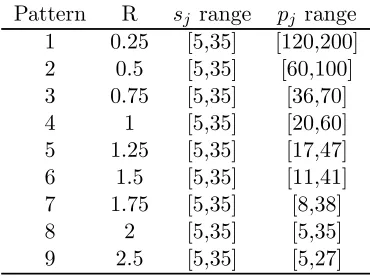
and 50 jobs. For each value of n, 9 separate patterns of data are tested. For each pattern, we generate 50 problem instances using different random seeds. We choose the ranges from which values of sj and pj are generated in such a way as to ensure that the average ratio between workloads on the server and processing machines over 50 instances approaches the corresponding value of R. Initialization time δ is standardized at value 1. The initial experiments indicate that no further dimensionality is required. Table 1 presents a summary of input test data.

Pattern R sj range pj range 1 0.25 [5,35] [120,200] 2 0.5 [5,35] [60,100] 3 0.75 [5,35] [36,70] 4 1 [5,35] [20,60] 5 1.25 [5,35] [17,47] 6 1.5 [5,35] [11,41] 7 1.75 [5,35] [8,38] 8 2 [5,35] [5,35] 9 2.5 [5,35] [5,27]

Table 1: Summary of generated data

Note that different patterns in Table 1 define different correlations between values ofsj and pj for individual jobs. For the first 3 patterns with lower values of R, we can observe a clear dominance of processing operations over setup operations for all jobs which makes the processing stage a bottleneck in the system. As R increases, the number of jobs for which sj > pj grows, and the server becomes a bottleneck. Patterns with R ≥1 represent mixes of jobs with different proportions of dominating setup and processing operations.

0.00 0.20 0.40 0.60 0.80 1.00 1.20 1.40 1.60

0 1 2 5 δ

Dav

(SC

) (%

)

R=0.5 R=1.5

Figure 7: Effect of changingδ on the performance of algorithmCS

5.2

Initial experiments

Our initial computational experiments to identify the significance of parameters are de-scribed below. We focus upon two aspects of problem instances: the relative times of setup and processing of samples, and the significance of initialization time. The experimental results and conclusions are outlined for each below. All initial experiments were conducted upon the full range of setup and processing times and number of jobs employed in thefinal benchmark dataset.

We generated datasets in which setup timessj and processing timespj are taken from different ranges. Two sets of scenarios were created in which either the setup operations or the main processing operations of jobs were dominant. We also considered a range of “mixed”datasets with different proportions of jobs with dominating setup component and jobs for which main processing operations were longer than their setup operations. The analysis of the problem structure indicated that the relative workload between the primary parallel machines and the setup machine was probably a key factor in determining the potential gain from batching jobs. Our initial computational experiments confirmed this. We therefore selected patterns of data characterized by the value of the ratio R between the total load WS of serverS and average loadWP of processing machines A and B, i.e.

R= WS

WP

,

where

WS= n

X

j=1

sj andWP =

1 2

n

X

j=1

(pj+δ).

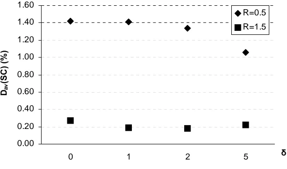
In our initial experiments for 10 jobs and different values ofR,we tested the procedure with no batching (algorithm NB) and algorithm CS for δ = 0,1,2 and 5, keeping setup and processing times of jobs unchanged. The ranges for sj and pj were selected in such a way as to ensure that min

Figure 7 shows the average performance of algorithm CS for 10 jobs, different values of δ

and R= 0.5and1.5. We can notice that algorithmCS produces high quality schedules for all tested values ofδ. In fact, increasingδby a certain amount∆leads to the increase of the makespan values produced by algorithm NB by n∆/2 for most instances of the problem. For both algorithmCS and branch and bound the magnitude of makespan increase usually lies in the range[∆,2∆]. Moreover, increasingδdoes not change the structure of schedules (i.e. the allocation of jobs to the machines and their partition into batches) constructed by algorithm CS and branch and bound. The reason for this is that δ is small relative to the lengths of setup and processing operations of jobs. Therefore, in what follows we will discuss only the results forδ = 1.

5.3

Results for benchmark datasets

For each pattern of data and each number of jobs, we compare the schedules constructed by the algorithm NB to those produced by algorithm CS. In addition, we calculate the optimum makespan obtained by branch and bound algorithm described in subsection 4.4. The comparative performance of the algorithms is summarized in Table 2. We use the following notation in the table:

Dav(H) — average percentage deviation (over 50 runs) of makespan values produced by algorithm H from the optimal makespans, for H=N B orCS;

Nopt(CS) — number of runs (out of 50) when the optimal solutions (or a surrogate in exceptional cases) were found by algorithm CS.

The CPU times required for a single run of algorithmCS are well under 1 second, while branch and bound algorithm may take long hours for certain runs especially when n= 50

and the ratio R is high. Note that the running time of the branch and bound algorithm was therefore restricted to 6 hours. For n = 50 and R >1,branch and bound was often unable to finish in such a time limit and the best solutions found in 6 hours were recorded instead of the optimal ones. Therefore, two values, separated by slash, are given in column

Nopt(CS)in cells corresponding ton= 50andR >1.Thefirst value represents the number of optimal solutions found by algorithmCS (either by reaching the lower bound or proven by branch and bound algorithm) while the second one shows the number of runs when branch and bound has not improved solutions found by algorithm CS within 6 hours time limit.

Our main observations are the following.

Pattern R n Dav(N B)(%) Dav(CS)(%) Nopt(CS) 1 0.25 10 12.03 0.69 27

25 13.47 1.06 2 50 14.00 0.49 2 2 0.5 10 20.85 1.41 25

25 24.93 1.41 6 50 25.83 0.86 0 3 0.75 10 26.61 1.27 22

25 33.87 1.67 8 50 38.72 1.34 2

4 1 10 29.00 0.80 35

25 39.03 1.35 15 50 45.22 1.33 1 5 1.25 10 25.31 0.53 38

25 35.65 0.70 25 50 39.26∗∗ _0.33∗∗ _17/12∗ 6 1.5 10 19.63 0.19 47

25 25.80 0.22 40 50 28.74∗∗ 0.00∗∗ 28/20∗ 7 1.75 10 16.89 0.14 46

25 21.50 0.08 45 50 23.24∗∗ _0.02∗∗ _32/16∗

8 2 10 14.65 0.06 46

25 15.51 0.01 48 50 17.78∗∗ 0.02∗∗ 40/9∗ 9 2.5 10 8.56 0.01 49

25 10.21 0.05 46 50 11.68∗∗ 0.00∗∗ 44/6∗ ∗ _{Number of runs when branch and bound did not improve heuristic solution}

within 6 hours

∗∗ _{Thefigure is based on complete and terminated runs of branch and bound}

0.00 0.20 0.40 0.60 0.80 1.00 1.20 1.40 1.60 1.80

0.25 0.5 0.75 1 1.25 1.5 1.75 2 2.25 2.5

R Dav

(C

S

) (

%

)

Figure 8: Performance of algorithmCS in relation to relative server workload, for 25 jobs

2. Effects of the relative workload between server and primary machines, R. Figure 8 summarizes our analysis and shows the dynamics in results produced by the algorithm as the ratio R raises, for problem instances with 25 jobs. Similar patterns can be observed for 10 and 50 jobs. Note that the “hardest” instances for the algorithm are those corresponding toR= 0.75. It appears that if the bottleneck is at the processing stage, algorithmCS performs better for problems with the greater difference between the processing and setup times of jobs (i.e. problems with lower R).

For R < 1, machines A and B are the bottleneck machines. Therefore balancing workloads and avoiding idle intervals as much as possible are the key factors for constructing a good schedule and uninterrupted load of server S is less important. Figures for Nopt in Table 2 show that algorithm CS finds optimal solutions only occasionally for instances with a greater number of jobs. This is also much the case for instances with R = 1 where there is no clear bottleneck stage and values of

LB1 and LB2 are very close to each other. Our investigation showed that optimal schedules found by branch and bound algorithm often contain a few idle intervals on machine S. On the other hand, algorithm CS only produces schedules with either no idle time or with a single idle interval on machine S at the end of the schedule. Therefore, a schedule constructed by algorithm CS can be potentially improved by splitting large batches and redistributing the jobs between machines A and B which synchronizes completion times of the last jobs on both machines.

with a better makespan, which provides extra evidence of the strong performance of algorithm CS.

3. Effects of increasing the number of jobs. Increasing the number of jobs makes the problem ISP more difficult to tackle. Comparing the number of optimal solutions

Nopt(CS) found by algorithmCS forn= 10,25 and 50 for each value of R, we can observe that Nopt(CS) decreases as the value ofn is growing.

5.4

Experiments with laboratory data

In this section, we illustrate the advantage of our approach in a real-world setting. We report the results of computational experiments on data provided by the microbiology laboratory. The current practice which predominates at the pipetting stations in the laboratory is that of initializing one sample at a time. This practice is replicated by the “no batching” algorithm,NB. We therefore compare the behaviour of our algorithmCS on the given data, to that of algorithmNB. The laboratory is equipped with three identical pipetting stations, although generally only two of them are in operation. We therefore run our experiments both for two and three parallel machines.

Historical data reflecting daily demand for testing were provided by the laboratory for 5 different days. A short summary showing the nature of the data is given in Table 3. Since the real sequences in which samples enter the testing process were not recorded by the laboratory, we generated 10 random sequences for each dataset.

Day Number Total number Workload of test suites of test samples,n ratio,R

1 21 573 1.45

2 22 441 1.65

3 31 570 1.58

4 19 502 1.45

5 29 556 1.56

Table 3: Summary of the laboratory data

Each test sample (considered as a job in our problem formulation) arriving to the pipetting stage has to undergo a certain number of microbiological tests which form its test suite. The jobs associated with a given test suite require the same labelling and pipetting times (i.e. setup and processing times, respectively) while these times usually differ between test suites. There are a number of “standard” test suites which are assigned to the majority of test samples entering the process each day. On the other hand, test samples with certain test suites may be absent in some days. Table 3 shows the variety in the number of test suites and in the total number of test samples, n, for 5 days.

Total Makespan (h:mm) Savings from Day labelling with no batching with batching (CS) batching jobs (%)

time average max average max min average max 1 5:56 7:47 7:50 5:57 5:58 23.2 23.5 24.1 2 3:47 4:41 4:42 3:47 3:48 18.2 18.9 19.5 3 4:42 5:56 5:57 4:43 4:44 20.3 20.6 20.8 4 5:48 7:46 7:49 5:49 5:50 24.7 25.1 25.6 5 4:40 5:56 5:57 4:41 4:42 20.5 20.9 21.2

Overall 18.2 21.8 25.6

Table 4: Performance of algorithms for two pipetting stations

with labelling times exceeding pipetting times and vice versa in each dataset. Figures from the last column of Table 3 suggest that the labelling machine is a bottleneck. Therefore, we can expect very strong outcomes from algorithmCS for such a scenario (see results and discussion in the previous section).

The results of running algorithms NB and CS for laboratory data and two pipetting stations are summarized in Table 4. All minimum, maximum and average figures in the tables are taken over 10 runs of each algorithm. Due to the large number of jobs in each dataset, running the branch and bound algorithm is impractical. We therefore use lower bounds to assess the quality of schedules. Since labelling machine is a bottleneck, lower bound LB1is most appropriate. The main component of LB1 is the total labelling time, which is given in the second column of Table 4.

The advantage of coordinated scheduling strategy with batching lying behind algorithm

CS over “no batching” strategy is evident from Table 4. The savings for two pipetting stations are in between 1 and 2 hours, averaging 22%. The minimum time savings from using batching recorded in our experiments is about 18% while the maximum savings exceed 25%. Comparing the results of algorithm CS with the total labelling time, it can be seen that the difference is just 1 or 2 minutes over a day. This difference is largely accounted for by the pipetting time of the last job. Therefore, the performance of algorithm CS cannot, in this context, be improved upon.

The effect of the sequence in which test samples are presented, is indicated by the range of outcomes for the 10 randomly generated sequences within each day’s dataset. The data from the laboratory indicate that such a difference is usually under 2 minutes, which is not significant relative to the magnitude of the makespans. Thus, the results suggest that sequencing test samples is not an important issue for the micro-biology laboratory.

deploy an additional pipetter. We therefore also testedNB for 3 pipetting stations, against the generalized versions of the CS algorithm for completeness. However, algorithm CS

with 2 pipetters still outperforms algorithm NB even with 3 pipetters for all instances of the problem. Indeed, the average time saving is about 3.5% in makespan in addition to the saving of 1 member of staff at the pipetting stations. Note that a single run of algorithm

CS on real data takes less than a second for two pipetting stations and does not exceed 1.5 seconds when 3 pipetting stations are used.

The above results illustrate the benefits of the batching strategy of algorithm CS. It creates the potential for raising the productivity of the laboratory by over 20%, by accom-modating an increased number of test samples processed in the laboratory during a day. Moreover, in current circumstances, the batching strategy should lead to savings in running costs of the laboratory, by eliminating the requirement for a third pipetter at any time.

6

Conclusions

The scheduling problem ISP studied in this paper has been identified at a particular stage of a complex technological process of food testing in the microbiological laboratory. The problem is of a very specific nature. It can be considered as a chain-reentrant two-stage hybridflowshop with parallel primary machines at thefirst stage and a single machine at the second stage with the additional requirement that the first and the last operations of each job should be performed by the same primary machine. To the best of our knowledge, hybrid reentrant shop problems have not been studied in the literature before. The closest problems in the literature, which share some common features are the problems of scheduling in a reentrant shop [8] and of scheduling on parallel machines with a common server [1]. We showed that the ISP problem is NP-hard even if the sequence of jobs is fixed. We developed a heuristic algorithm based on a simple strategy of initializing jobs in batches on the primary machines. Our heuristic avoids unnecessary idle times on the machine at the second stage (server) and provides balanced workloads on primary machines. These two features make our algorithm able tofind optimal or near optimal schedules in different production scenarios, both when the primary machines and when the server create the bottleneck in the system. We also show that our batching strategy is much more efficient than the strategy with no batching currently used in the laboratory. Adopting batching of jobs in practice may increase productivity of the production line and provide savings in the running costs of the company. Estimates are put at a saving of 1 member of staffor at 22% potential increase in productivity.

Acknowledgements

References

[1] Hall NG, Potts CN, Sriskandarajah C. Parallel machine scheduling with a common server. Discrete Applied Mathematics 2000;102:223-43.

[2] Brucker P, Dhaenens-Flipo C, Knust S, Kravchenko SA, Werner F. Complexity results for parallel machine problems with a single server. Journal of Scheduling 2002;5:429-57.

[3] Kravchenko SA, Werner F. Parallel machine scheduling problems with a single server. Mathematical and Computational Modelling 1997;26:1-11.

[4] Abdekhodaee AH, Wirth A. Scheduling parallel machines with a single server: some solvable cases and heuristics. Computers and Operations Research 2002;29:295-315.

[5] Abdekhodaee AH, Wirth A, Gan H-S. Scheduling two parallel machines with a single server: the general case. Computers and Operations Research 2006;33:994-1009.

[6] Glass CA, Shafransky YM, Strusevich VA. Scheduling for parallel dedicated machines with a single server. Naval Research Logistics 2000;47:304-28.

[7] Morton TE, Pentico DW. Heuristic scheduling systems: with applications to produc-tion systems and project management. John Wiley & Sons, New York, 1993.

[8] Wang MY, Sethi SP, van de Velde SL. Minimizing makespan in a class of re-entrant shops. Operations Research 1997;45:702-712.

[9] Drobouchevitch IG, Strusevich VA. A heuristic algorithm for two-machine re-entrant shop scheduling. Annals of Operations Research 1999;86:417-439.

[10] Potts CN, Kovalyov MY. Scheduling with batching: a review. European Journal of Operational Research 2000;120:228-49.

[11] Johnson SM. Optimal two- and three-stage production schedules with setup times included. Naval Research Logistics Quarterly 1954;1:61-68.

Appendices

A

Consistent and inconsistent batching

Consistent batching on a primary machine means that a new batch can not be initialised on a primary machine before all jobs from the previous batch are processed on that machine. A requirement for batch consistency is imposed by the company for quality assurance purposes. In this paper, we consider only the class of schedules with consistent batches.

1 2 3

A

B

1 2

3

S 4 5

4

5 1 2

3 4

5

1 2 3

A

B

1

2 3

S 4 5

4

5

1

2 3

4

5

1 2 3

A

B

1

2 3

S 4 5

4

5

1

2 3

4

5

a) Cmax= 16 b) Cmax= 15 c) Cmax= 15

Figure 9: Optimal schedules: a) for the class with consistent batches; b),c) when inconsis-tent batching is allowed

Consider the instance of the problem with n = 5, δ = 1, s = (sj) = (2,2,2,2,2) and

p= (pj) = (2,3,3,6,3).Figure 9 shows the optimal schedule for the class of schedules with only consistent batching (Figure 9a) and two examples of optimal schedules for a wider class of schedules where inconsistent batching is allowed (Figures 9b and 9c).In schedule b) job 5 is initialised as the first job of a new batch in between processing operations of jobs 2 and 3 from the previous batch. In schedule c) all initialisation operations for two consecutive batches on each machine are performed before the start of the processing operation of the first job from thefirst batch on that machine. Observe that both schedules with inconsistent batching have better makespans than the schedule with consistent batching. However, this is not necessarily the case for other instances of the problem. For example, adding job 6 with s6 = p6 = 2 to the last batch on machine A in schedule a) does not increase the

makespan for the new schedule with 6 jobs, and this schedule can not be improved by using inconsistent batching. It would be interesting to determine the conditions which make inconsistent batching advantageous. We leave this question for future research.

B

Pseudocodes of algorithm

Basic(1)

and its modi

fi

cations

In this appendix, we itemize the steps required to implement the basic batching strategy

Basic(1) and its modifications, Basic(i) and Repair, described in Section 4. The analysis of time complexity of the algorithms is also presented.

B.1

Algorithm

Basic(1)

Algorithm Basic(1)

1. Initialization.

1.1. Setα:= 0,β := 0,γ:= 0. {set machine availability times to zero}

1.3. Assign jobjto machineAby scheduling thefirst two operations of jobj(keeping the last operation unscheduled until a batch is completed):

I_jA:=α, α:=α+δ,

T_jS := max_{α, γ_}, C_jS :=T_jS+sj, γ:=CjS.

(12)

1.4. SetjF irst:= 1.{store the index of the first job in a batch}

2. While j < n {consider each unscheduled job}

j:=j+ 1.

2.1. If jobj₋1 was assigned toA and γ < β+δ, then

Addj to the last batch on machineAby scheduling the first two operations of jobj in accordance with (12) (keeping the last operation unscheduled until a batch is completed).

2.2. If jobj₋1 was assigned toA and γ_≥β+δ, then

2.2.1. {complete the current batch on A by scheduling its last operations} For =jF irsttoj₋1

TA_{:= max}©_{α, C}Sª_{, α:=T}A_{+p .} EndFor

2.2.2. Assign j as thefirst job of a new batch on machine B by scheduling the first two operations of that job (keeping the last operation unscheduled until a batch is completed):

I_jB :=β, β:=β+δ,

T_jS := max_{β, γ_}, C_jS :=T_jS+sj, γ:=C_jS.

2.2.3. Set jF irst:=j.

2.3. If jobj₋1is completed on B and γ < α+δ, then Addj to the last batch on machine B as for 2.1.

2.4. If jobj₋1 is completed on B and γ_≥α+δ, then

Complete previous batch on machineB and start a new batch on machineA

with jobj (without incurring an idle time on machineS) as for 2.2.

EndWhile

3. Complete the last batch by scheduling its main processing operations on machine A

orB as for 2.2.1.

4. Return resulting schedule σ(1),Cmax

¡

σ(1)¢= max_{α, β_}.

B.2

Algorithm

Basic(i)

Algorithm Basic(i)

1. Initialization.

1.1. Setα:= 0,β := 0,γ:= 0. {set machine availability times to zero}

1.2. {assign thefirst i jobs to machine A}.

Forj= 1toi

Assign jobj to machineA as in step 1.3 ofBasic(1).

EndFor

1.3. SetjF irst:= 1.{store the index of the first job in a batch}

2-3. The same as steps 2 and 3 of algorithmBasic(1).

4. Return schedule σ(i),Cmax¡σ(i)¢= max{α, β}.

Similar to Basic(1), algorithm Basic(i) has a linear time complexity and worst case performance ratio of 2.

B.3

Algorithm

Repair

Algorithm Repair

Input: schedule σ(i) constructed by algorithmBasic(i)

1. If Cmax

¡

σ(i)¢=δ+Pn_j=1sj+pn,then STOP (as scheduleσ(i) is optimal).

2. Set C[i]:=Cmax

¡

σ(i)¢, σ[i]:=σ(i).

Find the critical batch in schedule σ(i).

Let jcr be the first job in that batch andq be the size of the critical batch.

3. For k= 0toq₋2

3.1. Start to construct scheduleσ with the partial schedule ofσ(i) _{consisting of jobs}

1,2, . . . , jcr.

Schedule the next kjobsjcr+ 1, . . . , jcr+k in the same batch as jobjcr.

3.2. Schedule jobjcr+k+ 1on the alternative machine, starting a new batch on that machine.

3.3. Construct the remainder of schedule σ by assigning remaining jobs

jcr + k+ 2, . . . , n to the machines A and B using the strategy described in steps 2-3 of algorithm Basic(1).

SetC[i]:=Cmax(σ), σ[i]:=σ.

EndFor

4. Return σ[i], C[i].

Steps 1-2 of algorithmRepair requireO(n)time. Since the last batch containsq_≤n₋1

jobs, Step 3 is performed no more thann₋2times. In each iteration theO(n)-time algorithm

Basic is called. Thus the overall time complexity of algorithm Repair is O(n2).

C

Approximation bound

Theorem 2 For problem ISP, algorithm Basic(1) has a tight worst case bound of 2.

Proof. We show that for scheduleσ(1)constructed by algorithmBasic(1)the following inequality holds:

Cmax

¡

σ(1)¢ Cmax(σ∗) ≤

2,

where Cmax(σ∗) is the makespan of an optimal schedule.

In any schedule there always exists at least one job, called critical, which starts on the main processing machine exactly at the time its labeling operation is completed and is scheduled on a machine which achieves the makespan and has no idle time after this critical job. Letk be the latest job in sequence among all critical jobs in the scheduleσ(1)

and let N0 be the set of jobs which includes job k and all other jobs scheduled after job

k on the same machine. Observe that there can be several batches after the critical job and completion time of some job n0 _∈ N0, n0 _≤ n determines the makespan. Note that algorithmBasic(1) produces a schedule in which machineSprocesses the jobs without idle time. It follows that

Cmax

³

σ(1)´_≤δ+

k

X

j=1

sj+

X

j∈N0

pj +

¯

¯N0¯¯δ, (13)

where thefirst termδ corresponds to an idle time on machineS caused by the initialization time of the first job and the last term _|N0_|δ is the combined length of the initialization operations of the jobs from N0.

We use the following two lower bounds for the makespan of an optimal schedule:

Cmax(σ∗) ≥ LB0 =

1 2

⎛ ⎝

n

X

j=1

pj+nδ ⎞ ⎠,

Cmax(σ∗) ≥ LBk=δ+

k

X

j=1

sj +

1 2

⎛ ⎝

n

X

j=k

where the first inequality is based on the average load of machines A and B, while the second one uses the fact that in any schedule jobs k, . . . , n cannot start on machines A

or B earlier than the time δ +Pk_j=1sj and will occupy machine A or B for at least

1 2

³Pn

j=kpj + (n−k+ 1)δ

´

. Since N0 _{⊂ {}k, . . . , n_}, LB0 +LBk is no greater than the right hand side of (13) and hence

Cmax

³

σ(1)

´

≤2Cmax(σ∗).

Therefore Basic(1)is a 2-approximation algorithm.

To show that this bound is tight consider the following instance withn= 3jobs: δ =ε, s1 =s2 =s3 =ε, p1 = 1, p2 =T + 1, p3 =T. Algorithm Basic(1) produces the schedule

shown in Fig. 10 of length

Cmax

³

σ(1)´= 3ε+ 2T + 1,

where 3ε corresponds to initialization operation of job 1 and two setup operations of jobs

1 and 2. However, the schedule σ∗ illustrated in Fig. 11 has makespan

Cmax(σ∗) = 4ε+T+ 1.

12 3

A

B

1

S

2 3

2 3

1

T+1 T

Figure 10: A worst-case instance for algorithmBasic(1)

12 3

A

B

1

S

2

3 1

2

3

T

T+1

Figure 11: An optimal schedule for the worst-case instance

Schedule σ∗ is optimal since for small value of ε and large T both machine A and B

have equal workload. The ratio Cmax(σ (1)₎

FACULTY OF ACTUARIAL SCIENCE AND INSURANCE

Actuarial Research Papers since 2001

Report

Number

Date Publication

Title

Author

135. February 2001. On the Forecasting of Mortality Reduction Factors.

ISBN 1 901615 56 1

Steven Haberman Arthur E. Renshaw

136. February 2001. Multiple State Models, Simulation and Insurer Insolvency. ISBN 1 901615 57 X

Steve Haberman Zoltan Butt Ben Rickayzen

137. September 2001 A Cash-Flow Approach to Pension Funding. ISBN 1 901615 58 8

M. Zaki Khorasanee

138. November 2001 Addendum to “Analytic and Bootstrap Estimates of Prediction Errors in Claims Reserving”. ISBN 1 901615 59 6

Peter D. England

139. November 2001 A Bayesian Generalised Linear Model for the Bornhuetter-Ferguson Method of Claims Reserving. ISBN 1 901615 62 6

Richard J. Verrall

140. January 2002 Lee-Carter Mortality Forecasting, a Parallel GLM Approach, England and Wales Mortality Projections.

ISBN 1 901615 63 4

Arthur E.Renshaw Steven Haberman.

141. January 2002 Valuation of Guaranteed Annuity Conversion Options.

ISBN 1 901615 64 2

Laura Ballotta Steven Haberman

142. April 2002 Application of Frailty-Based Mortality Models to Insurance Data. ISBN 1 901615 65 0

Zoltan Butt Steven Haberman

143. Available 2003 Optimal Premium Pricing in Motor Insurance: A Discrete Approximation.

Russell J. Gerrard Celia Glass

144. December 2002 The Neighbourhood Health Economy. A Systematic Approach to the Examination of Health and Social Risks at Neighbourhood Level. ISBN 1 901615 66 9

Les Mayhew

145. January 2003 The Fair Valuation Problem of Guaranteed Annuity Options : The Stochastic Mortality Environment Case.

ISBN 1 901615 67 7

Laura Ballotta Steven Haberman

146. February 2003 Modelling and Valuation of Guarantees in With-Profit and Unitised With-Profit Life Insurance Contracts.

ISBN 1 901615 68 5

Steven Haberman Laura Ballotta Nan Want

147. March 2003. Optimal Retention Levels, Given the Joint Survival of Cedent and Reinsurer. ISBN 1 901615 69 3

Z. G. Ignatov Z.G., V.Kaishev

R.S. Krachunov

148. March 2003. Efficient Asset Valuation Methods for Pension Plans.

ISBN1 901615707

M. Iqbal Owadally

149. March 2003 Pension Funding and the Actuarial Assumption Concerning Investment Returns. ISBN 1 901615 71 5

M. Iqbal Owadally