Identifying drivers for the intra-urban spatial variability of airborne particulate matter components and their interrelationships

Identifying drivers for the intra-urban spatial variability of airborne

particulate matter components and their interrelationships

Hao Wu

, Stefan Reis

, Chun Lin

, Iain J. Beverland

, Mathew R. Heal

b_{Centre of Ecology&Hydrology, Bush Estate, Penicuik, Edinburgh, Midlothian, EH26 0QB, UK} c_{University of Exeter Medical School, Knowledge Spa, Truro, TR1 3HD, UK}

d_{University of Strathclyde, Department of Civil and Environmental Engineering, James Weir Building, 75 Montrose Street, Glasgow, G1 1XJ, UK}

h i g h l i g h t s

Peripatetic measurements of UFP, BC and PM2.5were taken in an urban environment.

Spatial variability in UFP and BC were much larger than in PM2.5.

UFP and BC were significantly correlated with traffic counts, while PM2.5was not.

PM2.5variability was largely determined by synoptic meteorological influences.

a r t i c l e i n f o

Article history:

Received 19 January 2015 Received in revised form 21 April 2015

Accepted 24 April 2015 Available online 25 April 2015

Keywords:

Black carbon Ultrafine particles PM2.5

Spatiotemporal variability Mobile measurements

a b s t r a c t

The aim of this work was to compare the variability in an urban area offine particles (PM2.5), ultrafine

particles (UFP) and black carbon (BC) and to evaluate the relationship between each particle metric and potential factors (local traffic, street topography and synoptic meteorology) contributing to the vari-ability. Concentrations of the three particle metrics were quantified using portable monitors through a combination of mobile and static measurements in the city of Edinburgh, UK. The spatial variability of UFP and BC was large, of similar magnitude and about 3 times higher than the spatial variability of PM 0.5-2.5(the PM size fraction actually quantified in this work). Highest inter-daily variability was observed for

PM0.5-2.5, which was approximately 2 times higher than inter-daily variability of BC and UFP. Elevated

concentrations of UFP and BC were observed along streets with high traffic volumes whereas PM0.5-2.5

showed less variation between streets and a footpath without road traffic. Both BC and UFP were significantly correlated with traffic counts, while no significant correlation between PM0.5-2.5and traffic

counts was observed. BC was significantly correlated with UFP, with significantly different regression slopes between working days and non-working days implying that the increased number of diesel powered heavy goods vehicles during working days contributed more to BC than to UFP. It is concluded that variations in BC and UFP concentrations were mainly determined by the nearby traffic count and varying background concentrations between days, while variation in PM0.5-2.5concentration was mainly

associated with regional sources. Thesefindings imply the need for different policies for managing human exposure to these different particle components: control of much BC and UFP appears to be manageable at local scale by restricting traffic emissions; however, abatement of PM2.5requires a more

strategic approach, in cooperation with other regions and countries on emissions control to curb long-range transport of PM2.5precursors.

©2015 The Authors. Published by Elsevier Ltd. This is an open access article under the CC BY license (http://creativecommons.org/licenses/by/4.0/).

1. Introduction

Evidence continues to accumulate of the adverse health impacts

of PM2.5, the mass concentration of airborne particulate matter

(PM) with an aerodynamic diameter of less than 2.5

m

2013). However, metrics of other characteristics of ambient PM

*Corresponding author. University of Edinburgh, School of Chemistry, Joseph Black Building, David Brewster Road, Edinburgh, EH9 3FJ, UK.

E-mail address:[email protected](H. Wu).

Contents lists available atScienceDirect

Atmospheric Environment

j o u r n a l h o m e p a g e : w w w . e l s e v i e r . c o m / l o c a t e / a t m o s e n v

http://dx.doi.org/10.1016/j.atmosenv.2015.04.059

including numbers of ultrafine particles (UFP, particles of diameter

<100 nm) and black carbon (BC) concentrations are emerging as

important in terms of their association with health effects (Heal

et al., 2012). A relevant issue is the extent to which UFP and BC concentrations vary within populated areas, since a shortcoming in many epidemiological studies is assumption of homogenous exposure within the study area. This might be plausible for

pol-lutants with less spatial variability but could result in significant

bias in exposure-response relationships for highly spatially variable

pollutants (Hoek et al., 2002). In this context, variables related to

the contribution of emissions from major roads (e.g. traffic

in-tensity, or distance to the road) are commonly identified as

sig-nificant predictors for a range of traffic-related air pollutants in

many studies applying land-use regression models (Hoek et al.,

2008), the validity of which might be influenced by the

underly-ing causes of the variability of different pollutants. Thus one of the aims of this work was to evaluate the extent to which potential factors affect the spatiotemporal variability of ambient BC, UFP and

PM2.5in an urban area. These factors include local traffic, street

topography and synoptic meteorology which, although recognised in the literature, have rarely been compared in terms of their

in-fluences on different metrics.

The three airborne particle metrics are closely related to traffic

in urban environments (HEI, 2010; Kassomenos et al., 2014;

Sandradewi et al., 2008) but, for PM2.5 in particular,

synoptic-scale meteorology also affects the dispersion and long-range

transport of secondary particles (Pinto et al., 2004). UFP

vari-ability is also subject to high intensity secondary formation

asso-ciated with strong solar radiation (Reche et al., 2011). Street

canyons, which are ubiquitous in many urban environments, introduce complex dispersion characteristics that further increase

the spatial variability of BC and UFP (Peters et al., 2014; Rakowska

et al., 2014). One limitation of inter- and intra-urban studies of

airborne particle concentrations is that the fixed-site

measure-ments on which they are based are rarely sufficient in number, and

thus in spatial coverage, to explore the variability of exposure to particles at street level. One way to monitor particle concentration at high spatiotemporal resolution is by use of mobile monitoring instruments, which has good prospects for wider application in the

assessment of human exposure to air pollution in the future (Steinle et al., 2013).

Both UFP and BC have received increasing interest in recent

studies (Patton et al., 2014; Ruths et al., 2014), as they can be

considered markers of a range of traffic-related particulate

pollut-ants. Therefore the relationships of UFP and BC with traffic volume

and composition need to be understood in order to correctly assign

exposure to traffic pollution in health studies. In the UK and many

other countries, PM2.5 and PM10are the only two regulated PM

metrics (AQEG, 2012). Given the increasing evidence for the

harm-fulness of UFP (WHO, 2013) with its ability to penetrate deep into

the airways (Knibbs et al., 2011), investigation on the relationship

between UFP and PM2.5can provide insight on the extent to which

current policy can effectively protect human health. Thus another aim of this work was to investigate the inter-relationships between

the different metrics of PM and their relationships with traffic.

In this work, pairs of portable instruments were used to

mea-sure PM0.5-2.5(used here as a measure of PM2.5), UFP number and

BC concentrations within the city of Edinburgh (Scotland) in two series of measurement campaigns in winter and in spring. Analyses of data from a combination of mobile and stationary measurements were used to evaluate possible causes of the variations in the concentrations of the different PM metrics.

2. Methods

2.1. Study design

BC, UFP and PM0.5-2.5concentrations were measured across the

south of the city of Edinburgh, UK (55.9N, 3.2 W, population

~480,000) in two separate campaigns using 2 units of the following instruments: microAeth AE51 (AE51), TSI 3007 Condensation Par-ticle Counter (CPC) and Dylos Corp. DC1700 (Dylos).

In the winter campaign, between December 2013 and January 2014, the measurements were conducted three times on Mondays and once on Sunday primarily near roadside by walking between

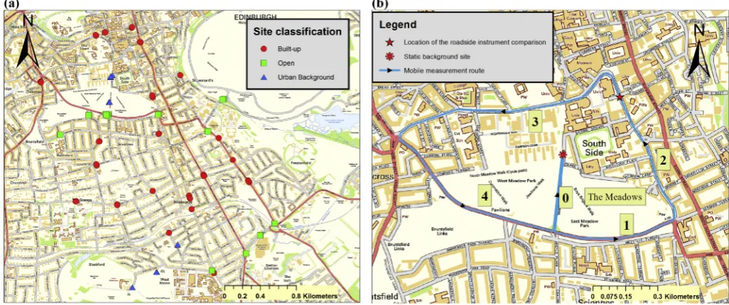
and pausing at designated sites (Fig. 1a). The sites were selected to

cover potential hotspots, urban background sites (at least 130 m from the nearest major road) and different street topographies

Fig. 1.(a) Location and classification of the static measurement sites. Streets with buildings on both sides are classified as built-up. Streets with buildings on only one side or no buildings on either side are classified as open. Background sites are at least 130 m away from the nearest major road. (b) Mobile measurement route and location of the contemporaneous background measurements. Segments of the mobile route are labelled from 0 to 4. Base map from Edina Digimap®.

(open or built-up) over an area of about 6 km2. In a typical walk, the measurements started at around 10:00 a.m. and proceeded through

the designated sites to thefinal location roughly in the order from

south to north and from east to west (Fig. 1a). At each site a 5-min

static measurement was conducted, during which the number and type of vehicles (car, van, heavy goods vehicle and bus) passing the observer were recorded. Throughout each walk, measurements for each pollutant were taken in parallel (with duplicate instruments) on both sides of the road. To evaluate the duplicate precision, inter-comparison between the pairs of instruments was conducted in a separate trial on Mon 3rd Feb 2014 from 10:00 a.m. to 12:00 p.m. by walking through the same route but with the duplicate instruments carried by one person. The weather conditions on this day were

similar to other measurement days (Supplementary Information

Table S1). Traffic characteristics are assumed to be similar to other Monday measurements.

In the spring campaign, between April and May 2014,

mea-surements were taken around a park area (~1 km2), referred to

locally as‘the Meadows’, focusing on understanding the

contribu-tions from traffic-related sources and local background sources to

BC, UFP and PM0.5-2.5on typical urban streets (Fig. 1b). The road on

the south edge of the Meadows had an annual average dailyflow of

13,272 vehicles in 2013 (Dft, 2015). The pollution level associated

with traffic was monitored by walking along a route surrounding

the Meadows. To measure temporal variation in the background concentrations, a duplicate set of instruments was located at a static site inside the route circuit during the collection of the mobile measurements. This background location had perpendicular dis-tance between 160 and 480 m to the three sides of the triangle

route (Fig. 1b). The measurements were conducted on one Sunday

andfive weekdays. On each day the mobile measurements started

together with the static measurements at the background site and

proceeded in the directions indicated inFig. 1b. Two trips were

carried out in the morning (~9e10 a.m.) and early afternoon (~1e2

p.m.) during each day, except for adverse weather conditions on one of the weekday afternoons. Other incomplete sets of mea-surements during each day were due to instrument faults. The

route of the mobile measurements was divided intofive segments

with different street topographies and traffic densities, as labelled

onFig. 1b. The total traf_fic passing the observer in the direction of

the route was counted for each segment. Trafficflow in the opposite

direction of the route is assumed to be similar. The duplicate in-struments were compared against each other during the last four measurement days by co-location for at least 20 min either at the

static background site or near a busy roadside (Fig. 1b). The

inclu-sion of both background and roadside sites was to cover a range of concentrations for the evaluation of duplicate instrument precision.

2.2. Instrumentation

The AE51 determines BC concentration from absorption of 880 nm laser light by particles continuously collected on a

glass-fibre filter. The CPC measures particle number concentrations of

particles between 0.01 and 1

m

scattering after condensing particles with super-saturated

iso-propanol vapour. Although UFP is usually de_fined as particles

smaller than 100 nm, since the number concentration is dominated

by ultrafine particles the measurement from the CPC can be

considered to represent UFP number concentration. The Dylos measures the particle number concentration using laser light

scattering technique in two size ranges,>0.5 and >2.5

m

particles between 0.5 and 2.5

m

study and are thus referred to as PM0.5-2.5. The use of the

termi-nology PM2.5elsewhere in this paper refers to the mass of all

par-ticles<2.5

m

In the winter campaign the time bases for the AE51, CPC and Dylos were 1 min, 1 s and 1 min, respectively. Because of the shorter duration of a trip in the spring campaign the resolution for the AE51

was increased to 30 s to ensure sufficient data points for each

segment. The Optimised Noise-reduction Averaging (ONA) algo-rithm was used to reduce the noise in the data recorded by the AE51 (Hagler et al., 2011). The ONA algorithm conducts adaptive time-averaging of the BC data, with the incremental light attenuation

(

D

time window of averaging. The

D

and 0.05 for winter and spring measurements, respectively, as a result of the different proportions of clean background areas and sampling resolutions in two campaigns. Negative values recorded after the smoothing were omitted from further analyses (consisting of ~5% of the whole data set), which mostly occurred when the

measured concentrations were<100 ng/m3.

Major axis (MA) regression analysis was carried out to test the equivalence between duplicate instruments, assuming that the

uncertainties in the duplicate instruments are similar (Warton

et al., 2006). A statistical summary of instrument

inter-comparison results is given in SITable S2. Correlations between

duplicate instruments were highly significant, however the 95%

confidence interval of the slopes for AE51 and CPC in spring

campaign and Dylos in both campaigns did not encompass unity. Therefore corrections based on the slope and intercept from the MA regression analyses were applied to the corresponding instruments to allow comparison between duplicate instruments.

2.3. Additional data

The average PM2.5concentrations measured by a TEOM-FDMS

instrument at the UK national network monitoring station St.

Leonards (55.945589N, 3.182186W) located 600 m to the east of

the Meadows during each set of measurements are summarised in SIFig. S1. The TEOM-FDMS is a reference-equivalent instrument for

quantifying gravimetric PM2.5for statutory purposes.

Meteorolog-ical data for the period of measurement for each day in both campaigns and for the period when instrument inter-comparisons were carried out in the winter campaign were obtained from a weather station on the rooftop of a seven storey building located

~3 km to the south of the Meadows (55.92N, 3.17W) and are

summarised inTable S1.

2.4. Data analyses

Reduced major axis (RMA) regression analysis was used to investigate the correlation between different pollutants, since the magnitudes of the data values and their uncertainties are not the

same for different instruments (Ayers, 2001). Given the skewed

nature of pollutant distributions, the non-parametric

Man-neWhitney U test and the KruskaleWallis test were used to

determine whether median concentrations differed significantly

between two and more than two samples, respectively. Data

ana-lyses were performed mainly using R software (R Core Team, 2014)

and sometimes Microsoft Excel. Back trajectory data was imported from pre-calculated trajectory data using the HYSPLIT trajectory

model via the “importTraj” function in openair (Carslaw and

Ropkins, 2012), an R package for air quality data analysis.

3. Results and discussion

3.1. Spatiotemporal variability of BC, UFP and PM0.5-2.5

Distributions of BC, UFP and PM0.5-2.5 concentrations in the

Fig. 2.Distributions of (a) BC, (b) UFP and (c) PM0.5-2.5concentrations measured on both sides of the road during each week in the winter campaign. The bold horizontal line denotes the median, and the box demarcates the interquartile range. The whiskers extend to the values 1.5 times the IQR on each side of the median. The PM0.5-2.5concentration measured by one of the Dylos instruments was corrected based on the statistics from MA regression analysis of instrument co-deployment during the winter campaign (Table S2). Side of road is defined with respect to the walking direction in the mobile measurements. The UFP concentrations in (b) are 1 min averages of the raw 1 s data.

H.

Wu

et

al.

/

Atmospheric

En

vironment

11

2

(20

15

)

306

e

31

6

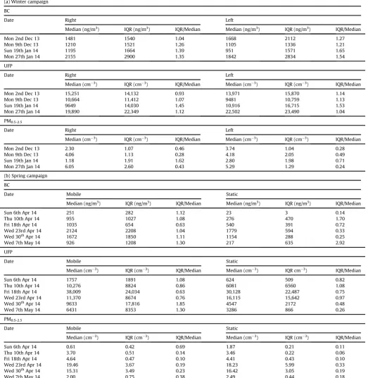
pollutant concentrations are highly skewed, especially for BC and UFP, so the interquartile range (IQR) is used to illustrate the varia-tion in distribuvaria-tion. Statistical summaries of the median and IQR for

measurements on both sides of the road are listed inTable 1a. BC

and UFP concentrations in spring campaign and PM0.5-2.5

concen-trations in both campaigns were corrected according to the MA

regression analyses results in Table S2to allow comparison

be-tween duplicate instruments. The ratio bebe-tween IQR and median is

used here as a metric of the spatiotemporal variability of each

pollutant during each measurement trip.Table 1a shows that BC

had the highest variability in the winter campaign (average IQR/ median ratio of 1.34), which is about twice as high as for the metric

with lowest variability, PM0.5-2.5(average IQR/median ratio of 0.56).

The difference in concentrations measured on two sides of the road

was not significant for BC and UFP as the median on one side of the

road was always within the IQR of the other side (Fig. 2). PM0.5-2.5

Table 1

The median, IQR and ratio between IQR and median on each day for BC, UFP and PM0.5-2.5for (a) winter and (b) summer campaign. Left and right side of the road is defined with

respect to the walking direction in the mobile measurements. Adjustment derived from MA regression analyses of instrument co-deployments (Table S1) was applied to one set of PM0.5-2.5data in both campaigns, and one set of BC and UFP data in the spring campaign.

(a) Winter campaign

BC

Date Right Left

Median (ng/m3_{) IQR (ng/m}3_{) IQR/Median Median (ng/m}3_{) IQR (ng/m}3_{) IQR/Median}

Mon 2nd Dec 13 1481 1540 1.04 1668 2112 1.27

Mon 9th Dec 13 1210 1521 1.26 1105 1336 1.21

Sun 19th Jan 14 1195 1664 1.39 951 1571 1.65

Mon 27th Jan 14 2155 2900 1.35 1842 2834 1.54

UFP

Date Right Left

Median (cm3) IQR (cm3) IQR/Median Median (cm3) IQR (cm3) IQR/Median

Mon 2nd Dec 13 15,251 14,132 0.93 13,971 15,870 1.14

Mon 9th Dec 13 10,664 11,412 1.07 9481 10,759 1.13

Sun 19th Jan 14 9649 14,030 1.45 10,916 16,715 1.53

Mon 27th Jan 14 19,890 22,349 1.12 22,502 23,490 1.04

PM0.5-2.5

Date Right Left

Median (cm3) IQR (cm3) IQR/Median Median (cm3) IQR (cm3) IQR/Median

Mon 2nd Dec 13 2.30 1.07 0.46 3.74 1.04 0.28

Mon 9th Dec 13 4.06 1.13 0.28 4.18 2.05 0.49

Sun 19th Jan 14 1.18 1.91 1.62 2.80 1.98 0.71

Mon 27th Jan 14 6.05 2.60 0.43 5.29 1.29 0.24

(b) Spring campaign

BC

Date Mobile Static

Median (ng/m3_{) IQR (ng/m}3_{) IQR/Median Median (ng/m}3_{) IQR (ng/m}3_{) IQR/Median}

Sun 6th Apr 14 251 282 1.12 23 3 0.14

Thu 10th Apr 14 955 1027 1.08 276 470 1.70

Fri 18th Apr 14 1035 654 0.63 540 391 0.72

Wed 23rd Apr 14 2124 2208 1.04 1779 594 0.33

Wed 30th_{Apr 14 1672 1850 1.11 1154 288 0.25}

Wed 7th May 14 926 1208 1.30 217 635 2.92

UFP

Date Mobile Static

Median (cm3) IQR (cm3) IQR/Median Median (cm3) IQR cm3) IQR/Median

Sun 6th Apr 14 1757 1891 1.08 624 509 0.82

Thu 10th Apr 14 10,276 8824 0.86 6081 6560 1.08

Fri 18th Apr 14 38,009 24,034 0.63 30,128 22,487 0.75

Wed 23rd Apr 14 11,370 8674 0.76 16,115 15,642 0.97

Wed 30th_{Apr 14 9633 17,816 1.85 4547 2172 0.48}

Wed 7th May 14 6431 8353 1.30 3286 866 0.26

PM0.5-2.5

Date Mobile Static

Median (cm3) IQR (cm3) IQR/Median Median (cm3) IQR (cm3) IQR/Median

Sun 6th Apr 14 0.61 0.42 0.69 1.87 0.21 0.11

Thu 10th Apr 14 3.70 0.51 0.14 3.46 0.22 0.06

Fri 18th Apr 14 4.64 0.47 0.10 4.41 0.43 0.10

Wed 23rd Apr 14 19.46 3.67 0.19 18.23 5.99 0.33

Wed 30th_{Apr 14 15.31 3.49 0.23 16.42 3.05 0.19}

showed noticeable difference in distributions between two sides of the road. However this may have resulted from the use of a single linear equation to correct the Dylos data. A 3-day comparison be-tween the duplicate Dylos instruments in an urban background

environment (55.92 N, 3.18 W) at the beginning of the winter

campaign (3rde 5th Dec 2013) showed a significantly different

slope from that derived from the inter-comparison at the end of the

winter campaign (3rd Feb 2014) (Table S2).Fig. S2suggests that the

relationship between the duplicate Dylos instruments might follow a different linear relationship between different days as indicated by the deviation of scatter points on one day from the main trend line. Due to lack of inter-comparison between the Dylos

in-struments during each measurement day, it is difficult to quantify

the genuine difference in PM0.5-2.5concentrations between the two

sides of road inFig. 2c. The discrepancies in the relationship

be-tween duplicate CPC and AE51 units on different days were

considered to be less significant than the Dylos, since the

correla-tion coefficients between CPC and AE51 units (r > 0.97) in the

mobile winter inter-comparison were much higher and the

gradients (0.98 and 0.97, respectively) were much closer to unity

than the Dylos equivalents (r¼0.90, gradient¼0.44) (Table S2).

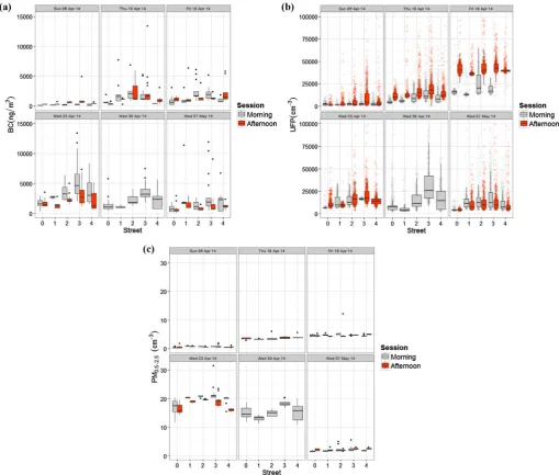
Distributions of BC, UFP and PM0.5-2.5 concentrations in the

spring measurements are summarised inFig. 3. Jittered points are

plotted for UFP to reveal the overlapping of large numbers of data

points. In order to discern the details of the boxes inFig. 3a and b,

BC and UFP concentrations greater than 15,000 ng/m3 and

100,000 cm-3, respectively, are not included. However, extremely

high concentrations were observed, extending to 50,000 ng/m3for

BC and 400,000 cm-3 for UFP. Elevated BC concentrations were

observed on streets with traffic (route segments 1e4) compared

with the footpath through an area of urban park (route segment 0). The median concentrations for each route segment also varied between different times of a day. Only on Thu 10th Apr 2014 were

BC concentrations not significantly different between morning and

noon sessions (ManneWhitney U test). BC concentration on Sun

6th Apr 2014 (median¼251 ng/m3) was significantly lower than on

weekdays (median¼1281 ng/m3) (one-tailed ManneWhitney U

test, P < 0.01), which is similar to findings in the winter

Fig. 3.Box plots for (a) BC, (b) UFP and (c) PM2.5concentrations grouped by different days and sessions in the spring campaign. Data visualisations as defined inFig. 2. Additional

jitter points are plotted inFig. 2b to reveal the extent of data in the outliers.

measurements.

The large range of outliers in the UFP distributions (Fig. 3b)

implied that UFP was greatly influenced by the emissions of nearby

traffic. Despite the fact that the outlier measurements on each

street were usually a factor 3 higher than their median, the dif-ference in the medians between streets was relatively small, sug-gesting that elevated levels due to occurrence of exhaust plumes only transiently affected the UFP concentration. Using ratios be-tween median concentrations on streets and on the footpath it was calculated that, on average, a pedestrian was exposed to 1.8 times higher concentration on streets than on the footpath for UFP, and 2.3 times higher for BC. The markedly high UFP level on Fri 18th Apr 2014 at noon was associated with the lowest wind speed, highest

solar_flux (Table S1) and relatively high O3concentration of ~70

m

m3(recorded at the St. Leonards UK national network monitoring

station) compared to other days. All these conditions are likely to have promoted secondary particle formation from photochemical

reactions (Reche et al., 2011).

The distribution of PM0.5-2.5concentrations (Fig. 3c) exhibited a

different pattern compared with the BC and UFP concentrations. The range of concentration on each street was smaller, and the relative variation in medians between streets within the same day

was lower. Only on Sunday and Wednesday 1 were PM0.5-2.5

con-centrations highly significantly different between footpath and the

streets (ManneWhitney U test,P<0.01), indicating that local traffic

is frequently not a dominant contributor to PM0.5-2.5concentrations

in the locations where measurements were made. Possible traf_fi

c-related sources to PM in this size range would be tyre and brake wear and road abrasion, but these are considered to contribute

relatively little to PM2.5(AQEG, 2012). Significant variation in PM

0.5-2.5concentrations was noticed between all spring working

sam-pling days (KruskaleWallis test,

c

implies that PM0.5-2.5 is more influenced by the regional sources

and meteorological conditions on a particular day rather than the

local traffic emissions. This is consistent with observations in other

cities, e.g. relatively low contribution (13%) to PM2.5 from local

traffic was also found in Paris (Skyllakou et al., 2014). Despite the

Dylos not measuring particles smaller than 0.5

m

vari-ation between days was in very good relative agreement with that

of the PM2.5 concentration measured by TEOM-FDMS at the St

Leonard's national network urban background site (SIFig. S1), i.e.

highest PM2.5levels on Mon 27th Jan 2014 in winter, and on Wed

23rd Apr 2014 and Wed 30th_{Apr 2014 in spring, and lower on}

Sundays in both campaigns.

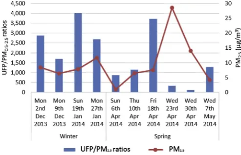
Assuming that UFP represents contribution from local traffic

sources, the ratio between median UFP and PM0.5-2.5approximates

the relative contribution of local sources to PM2.5concentration

during that day. However caution should be made in this inter-pretation since any photochemical new particle formation (e.g. Fri 18th Apr 2014 in spring campaign) may lead to overestimation of the relative level of local contribution compared to days when such an event is unfavourable. In the winter measurements, the highest

UFP/PM0.5-2.5ratio (3999), was associated with relatively low PM2.5

concentration (8

m

mea-surements, the highest ratio was on Fri 18th Apr 2014 (3715), which was about ten times the ratio on Wed 23rd Apr 2014 (349), despite

the fact the PM2.5concentration on Fri 18th Apr 2014 (~9

m

was only a third of that on Wed 23rd Apr 2014 (~27

m

noted that in both campaigns highest local contributions did not

coincide with the highest PM2.5concentrations. This observation

again indicates a strong regional component in PM2.5observed in

urban areas, as also noted byAQEG (2012).

Four-day air-mass back trajectories arriving at Edinburgh at 09:00 a.m. and 12:00 p.m. on each measurement day are plotted in SI Fig. S3. The trajectories associated with the highest PM2.5

concentrations in the winter and spring campaigns originated from North America and northern continental Europe, respectively.

However, the highest PM2.5concentration in winter coincided with

a relatively large contribution from local sources (UFP/PM0.5-2.5

ratio of 2682) suggesting that the high PM2.5on that particular day

may be mainly due to local emission sources. In contrast, the south-easterly trajectory originating from northern continental Europe (Fig. S3) was associated with high PM2.5concentrations and low

local contributions. It is notable that the PM2.5concentrations on

the days associated with relatively high local emissions were close to the Scottish annual air quality objective threshold concentration

for PM2.5of 12

m

the two days with PM2.5concentrations breaching the limit (Weds

23rd and 30thApr 2014 in spring,Fig. S1) had the largest regional

contribution. In the UK context, transboundary import of inorganic aerosol components resulting in high particle concentrations was

reported in a modelling study (Vieno et al., 2014).

The evidence presented here highlights that the effective

management of PM2.5in the UK may require international scale

cooperation in the control of emission sources. The good agreement between Dylos and TEOM-FDMS, together with the above analysis

on the potential sources of high PM2.5 episodes during each

campaign, confirm that the Dylos is capable of measuring elevated

PM2.5arising from both regional and local influences (Steinle et al.,

2015). However, this analysis does not reveal the contribution from

local traffic emission at street level. This is in line with thefindings

ofPrice et al. (2014)who showed that number concentration of particles greater than 262 nm was more closely related to meteo-rological conditions whilst UFP was more closely associated with

traffic variables. Nevertheless this work presents a novel approach

to apportioning PM2.5to local and regional sources by comparing

the relationship between UFP and PM2.5with the help of

back-trajectory analysis.

The IQR/median ratio was used to represent the variability of

each pollutant in the spring measurements (Table 1b), in which the

IQR/median ratio from the static measurements quantifies only the

temporal variation between different times of a day, and the ratio in

the mobile measurement reflects both spatial and temporal

varia-tion between different streets (with the former expected to be greater than the latter). Consistent with the observations in the winter measurements, the spatial variations of BC and UFP (average mobile IQR/median ratios of 1.05 and 1.08, respectively) were much

larger than spatial variations of PM0.5-2.5 (average mobile IQR/

Fig. 4.Ratios between median UFP and PM0.5-2.5concentrations and average PM2.5

median ratio of 0.29). The within-day variations of BC and UFP

(range of static IQR/median ratios 0.14e2.92 and 0.26e1.08,

respectively) were also generally larger than equivalent within-day

variations of PM0.5-2.5(range of static IQR/median ratios 0.06e0.33)

but were of varying magnitudes. This implies that changes in local

traffic counts and atmospheric conditions within a day have more

pronounced effects on variations in BC and UFP than on variations

in PM0.5-2.5. However PM0.5-2.5varied more between days (static

IQR/median ratio for the whole spring campaign of 3.27) than BC and UFP (equivalent ratios of 1.77 and 2.19, respectively). Collec-tively this evidence suggests that the variability of all three PM metrics is subject to the varying background concentrations. For BC and UFP in particular, the geographical locations, namely proximity

to traf_ficked roads, also contribute a signi_ficant part of the spatial

variability. Contrary to another study (Sullivan and Pryor, 2014),

which found that the spatial variability of PM2.5(defined as the

relative standard deviation for the mobile measurements on

different routes) was 2e3 times greater than the sub-daily

tem-poral variability (defined as the RSD for the measurements when

stationary), results from this study suggest that the spatial

vari-ability of PM0.5-2.5was of similar magnitude to the sub-daily

tem-poral variability. Possible explanations of this discrepancy include the larger geographical area in the former study, and the potential for bias from a few extremely high concentrations when using RSD rather than IQR as an indicator for variability.

3.2. Pollutant concentration in relation to street topography and traffic counts

To understand the relationship between traffic counts and the

pollutant concentration, reduced major axis (RMA) regression an-alyses were conducted between the mean of the concentrations on both sides of the road at each spot measurement in the winter

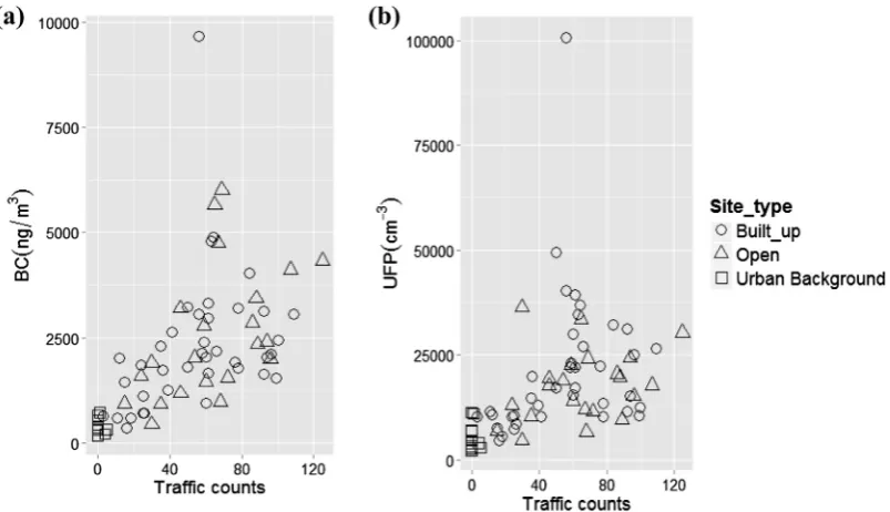
campaign and traffic counts.Fig. 5shows the scatter plots of BC and

UFP against traffic counts grouped by the classification of each site.

Correlations of 5-min average BC and UFP concentrations with

traffic counts were moderate and highly significant (r¼0.56 and

0.39, respectively,P<0.01,n¼72). PM0.5-2.5was not significantly

correlated with traffic counts (r¼0.17,n¼72).

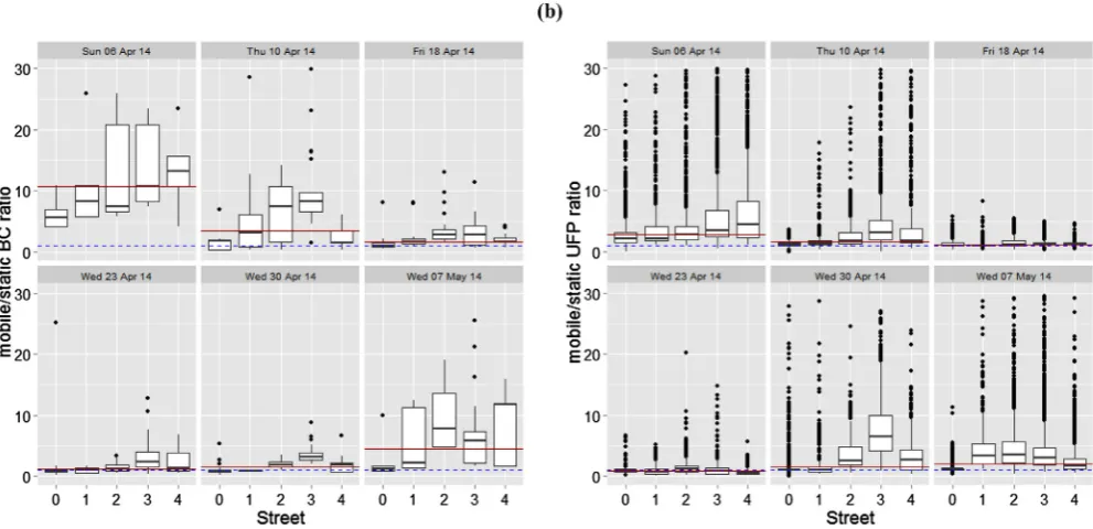
Ratios between mobile and static measurements in the spring campaign were calculated for each timestamp to represent the

elevation in the pollutant concentration due to traffic. The

distri-bution of the ratios for BC and UFP were grouped by streets and

plotted inFig. 6. Only ratios in the range 0e30 are shown inFig. 6to

avoid extreme values skewing the plots. Median mobile/static ra-tios are higher on Sun 6th Apr, Thu 10th Apr and Wed 7th May 2014 than on other days, an observation more pronounced for BC than for UFP. These days coincide with the days with higher wind speed (Table S1), which explains the greater contrast between roadside and background concentrations as the high wind speed facilitates the mixing of clean air at the background site while the immediate roadside concentration still stays at relatively high level. A sum-mary of the median values of the mobile/static measurement ratio

for each street and the traffic density on each street are tabulated in

Table 2. The data show a common pattern in the mobile/static ratios for BC and UFP: streets 2 and 3 had the highest median mobile/

static ratios. Considering that the traffic density in streets 2 and 3

were not the highest among all the streets, the difference in street topography is the most likely explanation of the greater mobile/ static ratios. Streets 2 and 3 are mostly characterised by street

canyons with aspect ratios in the range of 0.6e1.3, whereas streets

1 and 4 are beside the Meadows urban park with an open terrain. As a result, dispersion in streets 2 and 3 is likely to be reduced compared to dispersion in streets 1 and 4. Similar results were reported in a study in Hong Kong characterised by high-rise buildings, where notably elevated BC and UFP concentrations were observed in deep street canyons compared to an open road

although the trafficflow were significantly lower in street canyons

(Rakowska et al., 2014).

The correlation of averaged BC and UFP concentration with

traffic counts for each route segment was calculated in the spring

campaign. BC was again significantly correlated with traffic counts

(r¼0.45,P<0.01,n¼50), but UFP was not (r¼0.25,n¼48,

P ¼ 0.09). The lower correlation in spring compared to winter

campaign could be attributed to the fact that traffic counting on one

side of the street in spring campaign may not have represented

total traffic composition sufficiently. The low correlation between

traffic count and UFP may have been caused by the secondary

Fig. 5.Scatter plots of 5-min averaged (a) BC and (b) UFP concentrations vs. traffic counts at each measurement site in the winter campaign.

particle formation mentioned in Section3.1. This interpretation was supported by the increased correlation when the data from Friday

was excluded (r¼0.66,P<0.01,n¼39). Despite the moderate to

high correlation coefficients of BC and UFP with traffic counts found

in this study, mixed conclusions have been drawn in the literature

for the relationships between traffic and BC or UFP as a result of

characteristics of specific measurement sites, the consistency of

traf_fic_flow and the formation/transformation of particles governed

by environmental conditions (Kumar et al., 2008; Peters et al., 2014;

Price et al., 2014; Rakowska et al., 2014). Further investigation of

relationships between BC, UFP and traffic would provide beneficial

information to inform the potential use of nearby trafficflow data

to predict BC and UFP concentrations. Street topography effects on BC and UFP concentrations are similarly important for further investigation.

3.3. Correlation between BC and UFP

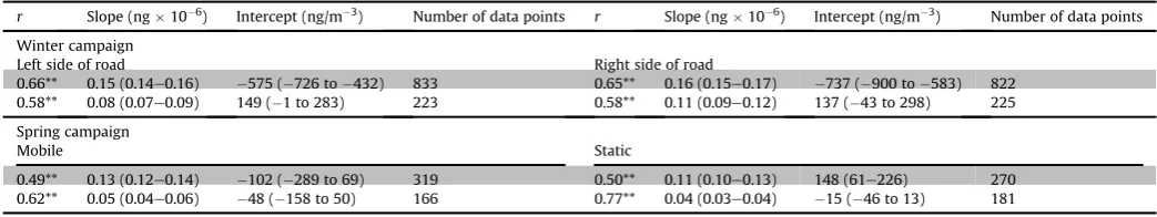
The correlations between BC and UFP were evaluated using RMA

regression. The results summarised inTable 3were calculated from

1-min averaged concentrations with BC as theyvariable and UFP as

thexvariable.

The correlations between BC and UFP during each week ranged

between 0.49 and 0.77 and in all cases were significant (P<0.01).

During working and non-working days, slope coef_ficients were not

significantly different between measurements taken on different

sides of the road in the winter campaign or between mobile and static measurements in the spring campaign. The agreement of the BC/UFP relationship between roadsides or between busy roads and local background suggests that BC and UFP concentrations

vary similarly as they disperse away from traffic sources. The

slopes on non-working days were significantly lower than the

slopes on working days, indicating a decrease in BC/UFP ratios on non-work days. This variation in the BC/UFP ratios was not only observed in the measurements taken near road but also in the static background measurements during the spring campaign. The reason for this variation in BC/UFP relationship is likely due to the decrease in heavy goods vehicles (HGV) on the road during the weekend as HGV had the lowest share on weekends (3.2%) compared with weekdays (~6.8%). This observation suggests that HGV contribute relatively more to BC than to UFP concentrations. Therefore a policy targeting on reduction of UFP may not be effective if it only focuses on restricting HGV. On the other hand policies aimed at reduction of BC should focus on controlling HGV emissions, which has direct implications for instance for the design and implementation of Low Emission Zones in urban areas. Considering that recent epidemiological studies suggested that BC was more strongly associated with harmful particle substances

than was the PM2.5mass (Grahame et al., 2014; WHO, 2013), traffic

control strategy targeting at the HGV may effectively contribute to Fig. 6.Distributions of mobile/static measurement ratios in different streets for (a) BC, and (b) UFP, in the winter campaign. Solid red lines denote the median mobile/static measurement ratio for each day. The dashed blue line denotes a ratio of one to highlight the elevated concentrations on streets. Measurements at the static background were corrected based on the MA regression analyses results inTable S2. (For interpretation of the references to colour in thisfigure legend, the reader is referred to the web version of this article.)

Table 2

Median ratios of mobile/static measurements in each street and the traffic density for each street.

Street Median of the mobile/static ratios for all the days (range of medians for each day) Mean traffic density (range of traffic density for each session) (traffic/km)

BC UFP

0 1.1 (0.9e5.6) 1.1 (1.0e2.2) 0

1 1.4 (0.9e8.3) 1.4 (0.7e3.4) 27 (16e38)

2 3.0 (1.2e7.8) 2.0 (1.2e3.5) 33 (24e42)

3 4.2 (2.4e15.8) 2.8 (0.9e7.0) 27 (18e35)

alleviation of population health burdens arising from urban air pollution.

3.4. Study limitations

This paper describes design and interpretation of a pilot study to investigate potential drivers for the spatiotemporal variability of different particulate matter components in the urban environment. It is recognised that it may be limited in terms of giving exhaustive

consideration and quantification of each individual driver on

pollutant concentration, particularly the complex influence of local

street topography. The absence of summer measurements could

mean that the influence of photochemical particle formation may

be underestimated (Ma and Birmili, 2015). Overall, however, this

study has demonstrated that careful experimental design and data interpretation of short-term mobile measurements can identify the important drivers governing different metrics of PM concentration,

and which also support findings in literature that use more

so-phisticated long term measurements.

4. Conclusions

Distributions of BC, UFP and PM0.5-2.5concentrations in the

ur-ban environment and the relationship between concentrations and

potential influences (local traffic, street topography and synoptic

meteorology) were studied through a combination of mobile and static measurements in the south of the city of Edinburgh, UK.

BC and UFP exhibited a high spatial variability in the urban

environment, roughly 3 times greater than that of PM0.5-2.5;

how-ever PM0.5-2.5had the highest inter-daily variability. Very high BC

and UFP concentrations were frequently measured at roadside and sometimes exceeded 3 times the street median concentration. However the median BC and UFP concentrations measured on the

streets were not greatly influenced by the frequent spikes and were

on average approximately double the median measured on the

footpath. PM0.5-2.5did not show a consistent elevated concentration

in the streets in comparison with the footpath. Both geographical locations and varying background concentrations had important

effects on the BC and UFP concentrations. Variation in PM0.5-2.5

concentrations was largely in_fluenced by regional sources,

although local sources also contributed to a lesser extent.

Both BC and UFP were highly correlated with traffic counts.

PM0.5-2.5showed very low correlation with the traffic counts.

Sig-nificant difference was found between the slopes of BC vs. UFP

regression analyses between working days and non-working days.

During non-working days the reduction of HGVflows results in a

decrease in the BC/UFP ratio, suggesting that HGV may contribute more to BC than to UFP concentrations. Therefore control of HGVs may be effective in reducing the negative health effects associated

with BC. PM2.5 was observed in a few instances to have a large

background component, the variability of which may not be well accounted for by only using local sources as indicators. Therefore international cooperation in control of emission sources is

impor-tant for PM2.5management in the UK. Furthermore, this study

in-dicates that the proximity to the road as a primary indicator for the assessment of exposure to air pollutants is highly dependent on the pollutant being considered.

Acknowledgement

Hao Wu acknowledges funding from the University of

Edin-burgh and the NERC Centre for Ecology&Hydrology (NERC CEH

project number NEC04544). The CPC and AE51 instruments were purchased under a NERC multi-institution grant (NE/1007822/1).

We thank Hugo Man for assistance in conducting the field

mea-surements and Christopher Malley for help in calculating back trajectories. We thank Defra for data from the UK AURN.

Appendix A. Supplementary data

Supplementary data related to this article can be found athttp://

dx.doi.org/10.1016/j.atmosenv.2015.04.059.

References

AQEG, 2012. Fine Particulate Matter (PM2.5) in the United Kingdom. Air Quality

Expert Group, UK Department for Environment. Food and Rural Affairs, London. PB13837.http://uk-air.defra.gov.uk/library/reports?report_id¼727.

Ayers, G.P., 2001. Comment on regression analysis of air quality data. Atmos. En-viron. 35, 2423e2425.

Carslaw, D.C., Ropkins, K., 2012. openairdAn R package for air quality data anal-ysis. Environ. Model. Softw. 27e28, 52e61.

Dft, 2015. City of Edinburgh [WWW Document]. Dep. Transp.eTraffic Counts. http://www.dft.gov.uk/traffic-counts/cp.php?la¼CityþofþEdinburgh.

Grahame, T.J., Klemm, R., Schlesinger, R.B., 2014. Public health and components of particulate matter: the changing assessment of black carbon. J. Air Waste Manag. Assoc. 64, 620e660.

Hagler, G.S.W., Yelverton, T.L.B., Vedantham, R., Hansen, A.D.A., Turner, J.R., 2011. Post-processing method to reduce noise while preserving high time resolution in aethalometer real-time black carbon data. Aerosol Air Qual. Res. 11, 539e546.

Heal, M.R., Kumar, P., Harrison, R.M., 2012. Particles, air quality, policy and health. Chem. Soc. Rev. 41, 6606.

HEI, 2010. Traffic-related Air Pollution: a Critical Review of the Literature on Emissions, Exposure, and Health Effects. Health Effects Institute.

Hoek, G., Beelen, R., de Hoogh, K., Vienneau, D., Gulliver, J., Fischer, P., Briggs, D., 2008. A review of land-use regression models to assess spatial variation of outdoor air pollution. Atmos. Environ. 42, 7561e7578.

Hoek, G., Meliefste, K., Cyrys, J., Lewne, M., Bellander, T., Brauer, M., Fischer, P., Gehring, U., Heinrich, J., van Vliet, P., Brunekreef, B., 2002. Spatial variability of

fine particle concentrations in three European areas. Atmos. Environ. 36, 4077e4088.

Kassomenos, P.A., Vardoulakis, S., Chaloulakou, A., Paschalidou, A.K., Grivas, G., Borge, R., Lumbreras, J., 2014. Study of PM10 and PM2.5 levels in three European cities: analysis of intra and inter urban variations. Atmos. Environ. 87, 153e163.

Knibbs, L.D., Cole-Hunter, T., Morawska, L., 2011. A review of commuter exposure to ultrafine particles and its health effects. Atmos. Environ. 45, 2611e2622.

Table 3

RMA regression analyses for 1-min averaged BC and UFP concentrations. The shading in the table represents the data collection period (grey: working days; white: non-working days). Left and right side of the road is defined with respect to the walking direction in the mobile measurements. ** indicates correlation at>99% significance.

r Slope (ng106) Intercept (ng/m3) Number of data points r Slope (ng106) Intercept (ng/m3) Number of data points

Winter campaign

Left side of road Right side of road

0.66** 0.15 (0.14e0.16) 575 (726 to432) 833 0.65** 0.16 (0.15e0.17) 737 (900 to583) 822

0.58** 0.08 (0.07e0.09) 149 (1 to 283) 223 0.58** 0.11 (0.09e0.12) 137 (43 to 298) 225

Spring campaign

Mobile Static

0.49** 0.13 (0.12e0.14) 102 (289 to 69) 319 0.50** 0.11 (0.10e0.13) 148 (61e226) 270

0.62** 0.05 (0.04e0.06) 48 (158 to 50) 166 0.77** 0.04 (0.03e0.04) 15 (46 to 13) 181

Kumar, P., Fennell, P., Britter, R., 2008. Measurements of particles in the 5-1000 nm range close to road level in an urban street canyon. Sci. Total Environ. 390, 437e447.

Ma, N., Birmili, W., 2015. Estimating the contribution of photochemical particle formation to ultrafine particle number averages in an urban atmosphere. Sci. Total Environ. 512e513, 154e166.

Patton, A.P., Perkins, J., Zamore, W., Levy, J.I., Brugge, D., Durant, J.L., 2014. Spatial and temporal differences in traffic-related air pollution in three urban neigh-borhoods near an interstate highway. Atmos. Environ. 99, 309e321.

Peters, J., Van den Bossche, J., Reggente, M., Van Poppel, M., De Baets, B., Theunis, J., 2014. Cyclist exposure to UFP and BC on urban routes in Antwerp. Belg. Atmos. Environ. 92, 31e43.

Pinto, J.P., Lefohn, A.S., Shadwick, D.S., 2004. Spatial variability of PM2.5 in urban areas in the United States. J. Air Waste Manag. Assoc. 1995 (54), 440e449.

Price, H.D., Arthur, R., BeruBe, K.A., Jones, T.P., 2014. Linking particle number con-centration (PNC), meteorology and traffic variables in a UK street canyon. Atmos. Res. 147e148, 133e144.

Rakowska, A., Wong, K.C., Townsend, T., Chan, K.L., Westerdahl, D., Ng, S., Mocnik, G., Drinovec, L., Ning, Z., 2014. Impact of traffic volume and composi-tion on the air quality and pedestrian exposure in urban street canyon. Atmos. Environ. 98, 260e270.

R Core Team, 2014. R: a Language and Environment for Statistical Computing. R Foundation for Statistical Computing, Vienna, Austria.http://www.R-project. org/.

Reche, C., Querol, X., Alastuey, A., Viana, M., Pey, J., Moreno, T., Rodríguez, S., Gonzalez, Y., Fernandez-Camacho, R., de la Campa, A.M.S., de la Rosa, J., Dall’Osto, M., Prev^ot, A.S.H., Hueglin, C., Harrison, R.M., Quincey, P., 2011. New considerations for PM, black Carbon and particle number concentration for air quality monitoring across different European cities. Atmos. Chem. Phys. 11, 6207e6227.

Ruths, M., von Bismarck-Osten, C., Weber, S., 2014. Measuring and modelling the

local-scale spatio-temporal variation of urban particle number size distribu-tions and black carbon. Atmos. Environ. 96, 37e49.

Sandradewi, J., Prevot, A.S.H., Szidat, S., Perron, N., Alfarra, M.R., Lanz, V.A.,^ Weingartner, E., Baltensperger, U., 2008. Using aerosol light absorption mea-surements for the quantitative determination of wood burning and traffic emission contributions to particulate matter. Environ. Sci. Technol. 42, 3316e3323.

Skyllakou, K., Murphy, B.N., Megaritis, A.G., Fountoukis, C., Pandis, S.N., 2014. Contributions of local and regional sources tofine PM in the megacity of Paris. Atmos. Chem. Phys. 14, 2343e2352.

Steinle, S., Reis, S., Sabel, C.E., 2013. Quantifying human exposure to air pollutione moving from static monitoring to spatio-temporally resolved personal exposure assessment. Sci. Total Environ. 184.

Steinle, S., Reis, S., Sabel, C.E., Semple, S., Twigg, M.M., Braban, C.F., Leeson, S.R., Heal, M.R., Harrison, D., Lin, C., Wu, H., 2015. Personal exposure monitoring of PM2.5 in indoor and outdoor microenvironments. Sci. Total Environ. 508, 383e394.

Sullivan, R.C., Pryor, S.C., 2014. Quantifying spatiotemporal variability offine par-ticles in an urban environment using combinedfixed and mobile measure-ments. Atmos. Environ. 89, 664e671.

Vieno, M., Heal, M.R., Hallsworth, S., Famulari, D., Doherty, R.M., Dore, A.J., Tang, Y.S., Braban, C.F., Leaver, D., Sutton, M.A., Reis, S., 2014. The role of long-range transport and domestic emissions in determining atmospheric secondary inorganic particle concentrations across the UK. Atmos. Chem. Phys. 14, 8435e8447.

Warton, D.I., Wright, I.J., Falster, D.S., Westoby, M., 2006. Bivariate line-fitting methods for allometry. Biol. Rev. 81, 259e291.

WHO, 2013. Review of Evidence on Health Aspects of Air PollutioneREVIHAAP

Project: Technical Report. World Health Organisation, Copenhagen, Denmark.