City, University of London Institutional Repository
Citation
:
Martinez-Miranda, M. D., Nielsen, B., Nielsen, J. P. and Verrall, R. J. (2011). Cash flow simulation for a model of outstanding liabilities based on claim amounts and claim numbers. ASTIN Bulletin, 41(1), pp. 107-129.This is the unspecified version of the paper.
This version of the publication may differ from the final published
version.
Permanent repository link:
http://openaccess.city.ac.uk/3803/Link to published version
:
Copyright and reuse:
City Research Online aims to make research
outputs of City, University of London available to a wider audience.
Copyright and Moral Rights remain with the author(s) and/or copyright
holders. URLs from City Research Online may be freely distributed and
linked to.
City Research Online: http://openaccess.city.ac.uk/ [email protected]
Cash flow simulation for a model of outstanding
liabilities based on claim amounts and claim numbers
Mar´ıa Dolores Mart´ınez Miranda
University of Granada, Campus Fuentenueva, 18071, Granada, Spain [email protected]
Bent Nielsen
Nuffield College, Oxford OX1 1NF, U.K. [email protected]
Jens Perch Nielsen
Cass Business School, City University London, 106 Bunhill Row, London EC1Y 8TZ, U.K.
and Richard Verrall
Cass Business School, City University, London [email protected]
6 September 2010
Abstract
In this paper we develop a full stochastic cash flow model of out-standing liabilities for the model developed in Verrall, Nielsen and Jessen (2010). This model is based on the simple triangular data available in most non-life insurance companies. By using more data, it is expected that the method will have less volatility than the cel-ebrated chain ladder method. Eventually, our method will lead to lower solvency requirements for those insurance companies that de-cide to collect counts data and replace their conventional chain ladder method.
1
Introduction
we consider the distributional properties of this model and compare it with the chain ladder model. It is to be expected that the additional information of the count triangle should lower the volatility of estimated reserves: when more information is available, the predictions should be better. We also note that the RBNS forecasts use the actual numbers of claims, and can therefore be considered to be based on a conditional model of the claim amounts, given the numbers of claims. On the other hand, the IBNR forecasts require, by definition, forecasts of the numbers of claims. We also examine in more detail some of the estimation issues associated with the model developed by Verrall, Nielsen and Jessen (2010).
The model of Verrall, Nielsen and Jessen (2010) separates the reporting delay from the payment delay from reporting to payment: the reporting delay is observed in the reported counts triangle and the delay observed in the paid triangle is a mixture of the reporting delay and the payment delay. The payment delay and the claims severity are estimated from a conditional model of the paid triangle given the counts triangle. In this paper, we exploit this new method in order to split the full stochastic cash flow into one cash flow related to the RBNS reserve and another related to the IBNR reserve. The RBNS reserve is predicted without modelling the counts but instead exploiting the fact that the reported counts give an advance warning of future payments. The IBNR reserve is constructed by first predicting the reported number of claims and then applying the same conditional model for payments given counts as outlined above. Thus, in this paper we construct bootstrap estimates of the predictive distributions total reserve and its split into RBNS and the IBNR reserves.
conditionally on the counts data. Recently, Bj¨orkwall, H¨ossjer and Ohlsson (2009b) have constructed conditional bootstrap estimators for such a sepa-ration method.
Section 6 contains the explanation of the bootstrap method for the model of Verrall, Nielsen and Jessen (2010). In sections 3,4 and 5 we summarise the model and explain some alterations in the set-up and estimation methods. The aim of this is to make the bootstrapping procedure as straightforward as possible to implement. It should be noted that the underlying structure of the model and the basic philosophy of the approach remain the same. In section 7, we consider some simulation studies which are designed to illustrate how the model behaves in general.
2
The data
This paper uses the same motor data as Verrall, Nielsen and Jessen (2010), which originates from the general insurer RSA and is based on a portfolio of motor third party liability policies. These data typically have long settlement delays, and the cashflow model in this paper is aimed at improved stochastic modelling of data of this type. The data available consists of two incremental run-off triangles of dimension m= 10, one for reported counts, Nij, and one for aggregated payments, Xij, where i= 1, . . . , m denotes the accident year and j = 0, . . . , m−1 is the development year. Collectively, we have data
N = {Nij,(i, j) ∈ I} and X = {Xij,(i, j) ∈ I} where I is the triangular index set
I ={i= 1, . . . , m, j = 0, . . . , m−1 with i+j = 1, . . . , m}.
The data are shown in Tables 1 and 2, respectively. The data for the ag-gregate paid claims have been inflation corrected using an inflation index depending on the calendar year i+j. This adjustment was carried out using an external economic inflation index before the data were supplied to the authors. It is not known when the payments aggregated as Xij were first reported.
3
The statistical model
i \ j 0 1 2 3 4 5 6 7 8 9 1 6238 831 49 7 1 1 2 1 2 3 2 7773 1381 23 4 1 3 1 1 3 3 10306 1093 17 5 2 0 2 2 4 9639 995 17 6 1 5 4 5 9511 1386 39 4 6 5 6 10023 1342 31 16 9 7 9834 1424 59 24 8 10899 1503 84 9 11954 1704 10 10989
Table 1: Run-off triangle of number of reported claims,Nij
i \ j 0 1 2 3 4 5 6 7 8 9
1 451288 339519 333371 144988 93243 45511 25217 20406 31482 1729 2 448627 512882 168467 130674 56044 33397 56071 26522 14346 3 693574 497737 202272 120753 125046 37154 27608 17864 4 652043 546406 244474 200896 106802 106753 63688 5 566082 503970 217838 145181 165519 91313
6 606606 562543 227374 153551 132743 7 536976 472525 154205 150564
8 554833 590880 300964 9 537238 701111
[image:5.595.188.421.124.230.2]10 684944
Table 2: Run-off triangle of aggregated payments, Xij
with a model for incurred counts. In this section, we give a summary of the model and describe a number of differences in the set-up and estimation which simplify Verrall, Nielsen and Jessen (2010) without making any significant changes to the overall structure.
3.1
The conditional model for payments given counts
The key feature of the cash flow model of Verrall, Nielsen and Jessen (2010) is to identify the payment delay through a conditional model for the payments
X given the reported counts N. The reported claims from accident year i
in section 4.2. The overall, but latent, number of payments in development year j is therefore
Nijpaid=
min(j,d)
X
k=0
Ni,jpaid−k,k. (1)
The observed aggregate payment in development year j is then
Xij =
Nijpaid X
k=1
Yij(k) (2)
where Yij(k) denotes an individual claim payment.
We assume that the delays are independent of the counts, and are as-sumed to take the values 0,1, . . . , d with probabilities p0, p1, . . . , pd, where
Pd
k=0pk = 1. In principle, these probabilities could depend on accident
year and development year, but in this paper we refrain from this further complication.
As in Verrall, Nielsen and Jessen (2010), it is assumed that the indi-vidual payments are independent of delays and counts and are identically distributed with expectationµand varianceσ2. While we recognise that this
assumption may be unrealistic, we leave possible extensions to other models for future work. The methodology is quite flexible about the distribution for individual payments. Verrall, Nielsen and Jessen (2010) used a mixed-type distribution which allowed for the possibility of zero claims, and we use this set-up in section 4.2 when examining the delay distribution. In section 6, we illustrate the bootstrap procedures using a simpler assumption that the payments are gamma distributed (with no allowance for the possibility of zero claims). In practice, additional external information may be available on (for instance) the frequency of zero claims and negative claims as well as on the tail behaviour of the claims.
The conditional expectation and variance of claims given the reported counts were computed in Verrall, Nielsen and Jessen (2010):
mij(N) = E(Xij |N) =
min(j,d)
X
k=0
Ni,j−kµpk, (3)
vij(N) = Var(Xij |N) =
min(j,d)
X
k=0
These formulas are used for the estimation of the parameters, and the con-ditional expectation (3) is used to calculate a point forecasts of the RBNS reserve (using the incurred counts) and of the IBNR reserve (using predicted counts).
3.2
The model for counts
The model for the counts N will be used for predicting the IBNR counts while it has no bearing on the predictions of the RBNS reserve. For the data in Table 1 a standard Poisson chain-ladder model seems reasonable. A generalisation could be to include a calendar effect as in Zehnwirth (1994) and the recent analysis in Kuang, Nielsen and Nielsen (2008a,b, 2010). Bryden and Verrall (2009) also discuss calendar year effects in the context of the chain-ladder technique.
The variables Nij are therefore assumed to be independently Poisson di-stributed with expectation
log{E(Nij)}=µij =αi+βj,
so thatαi is an accident year parameter andβj is a development year param-eter. The maximum likelihood analysis leads to the standard chain ladder analysis as shown by Kremer (1985), for example. Recently Kuang, Nielsen and Nielsen (2009) have revisited the maximum likelihood analysis and shown that the row sums and development factors of the chain ladder analysis are maximum likelihood estimators for the parameters.
4
Estimation
In this section, we summarise the estimation of the parameters, based on the theory of Verrall, Nielsen and Jessen (2010). We start by reviewing chain ladder estimation for the incurred counts. This is followed by a discussion of the estimation for the delay parameters ψk =µpk. Finally, estimators for the individual payment parameters µ and σ2 are given.
4.1
Chain ladder estimation of the model for counts
sums and the development factors,
Ri =
m−i X
k=0
Nik, Fℓ =
Pm−ℓ i=1
Pℓ j=0Nij
Pm−ℓ i=1
Pℓ−1
j=0Nij
, 1≤ℓ ≤m−1, (5)
are maximum likelihood estimators for the parameters ρi = E(Ri) and the
development factors, Φℓ, see Kuang, Nielsen and Nielsen (2009).
The fitted values are denoted byNijb , and for use later we define the ratios
b
Bj =Nij/b Nib0 =
(Fj−1)Qjk−=11Fk j ≥2, F1−1 j = 1,
1 j = 0,
(6)
which do not depend on the row indexi, see also Kuang, Nielsen and Nielsen (2009, eq. 14).
4.2
Estimating the delay and payment means
Considering next the triangle of paid claims, the delay parameters and the payment mean are estimated from the conditional model for the paymentsX
given incurred countsN as in Verrall, Nielsen and Jessen (2010). The idea is to estimate the parameters through a Poisson regression of payments X on incurred counts N using the conditional mean function mij(N) = E(Xij |N)
given in (3). The parameters ψk = µpk are then estimated by maximising the pseudo likelihood
ℓpseudo(ψ;X, N) = X i,j∈I
{Xijlogmij(N)−mij(N)}. (7)
Based on the estimatorsψkb ,k = 0, . . . , d the mean of the claims distribution and the delay probabilities are estimated by
b µ= d X k=0 b
ψk pkb =ψk/b µ.b (8)
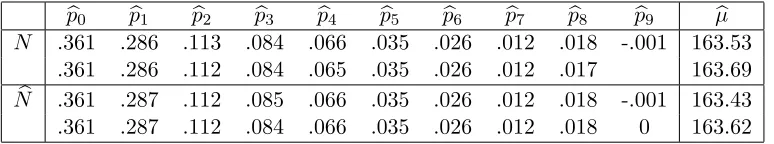
Table 3, first row of first panel, reports the estimates for the data in section 2.
b
p0 pb1 pb2 pb3 pb4 pb5 pb6 pb7 pb8 pb9 µb
N .361 .286 .113 .084 .066 .035 .026 .012 .018 -.001 163.53 .361 .286 .112 .084 .065 .035 .026 .012 .017 163.69 b
N .361 .287 .112 .085 .066 .035 .026 .012 .018 -.001 163.43 .361 .287 .112 .084 .066 .035 .026 .012 .018 0 163.62
Table 3: Pseudo likelihood estimators of the delay probabilities pk based on data in Tables 1, 2. Panel 1 uses actual counts with maximal delay of
d = m−1 = 9 and d = m−2 = 8, respectively. Panel 2 uses predicted counts and the analytic formula (in Row 2 the last entry is replaced by zero).
p9 1.3e-6 5.4e-3 0.018
[image:9.595.112.499.125.197.2]P(pb9 <0) 72% 33% 10%
Table 4: The frequency of zero estimates of p9 is simulated for different
values ofp9 using 1000 repetitions. The delay probabilities in the first column
were chosen asp =(0.360,0.288,0.111,0.083,0.066,0.035,0.025,0.013,0.016,1.3e-6). In the second column the last p9 was substituted by 5.4e−3 and p8 was
slightly modified so the pk’s sum to one. Finally, the third column considers
p=(0.182,0.164,0.145,0.127,0.109,0.091,0.073,0.055,0.036,0.018). The claims distribution considered in the three cases was a gamma (with mean µ = 204.91 and variance σ2 = 2589440) mixed with 20% zeros. The counts were
kept fixed as in Table 1.
practice, this may arise since the delay probabilities will tend to tail off so that for instance pm−1 will be close to zero, with the result that the estimate
may be negative in some cases. One response is to impose the restriction that the maximal delay is shorter, for instance d =m−2. Table 3, second row of first panel, reports the estimates for the motor data, and it can be seen that, for this particular data set, there is not much difference between the results. The relative differences are largest, up to 5%, for the longest delays, but in absolute terms the differences are modest, up to 0.1%.
We investigated the chance of negative estimates by simulation, and Table 4 reports the simulated probability that the analytic estimator of the longest delay ψ9 is negative for different values of ψ9. The probability of negative
be an issue in practice.
One approach to deal with negative delay estimates would be to use a constrained optimization routine to ensure that all estimators are non-negative. Having the subsequent bootstrap in mind we suggest a pragmatic estimator, which is numerically less intensive. If the sum of absolute values of negative ψkb is less than 1% of the sum of absolute values of all ψkb then the negative estimates are replaced by zero. If the sum of negative estimates is larger than this threshold it may be useful to investigate whether the paid data have special features such as many zeros.
4.3
Analytic estimation of delay parameters
Again keeping the bootstrap procedure in mind, we suggest an analytic esti-mator of the delay parameters as a numerically less costly alternative to the above iterative procedure. In this, we depart from Verrall, Nielsen and Jessen (2010). While the above estimation procedure conditions on the actual count data the idea of the alternative is to exploit a possible chain ladder structure for the counts data. We expect this to work well as long as the counts data do not deviate much from the chain ladder model, by for instance having a significant calendar effect. This analytic method only works whend=m−1, which is what is assumed in this section. In practice, it is necessary to check for negative delay parameter values and set these to zero, as discussed at the end of section 4.2.
Thus, the proposal is to replace the observed counts N in the pseudo likelihood (7) by the fitted counts Nb from a chain ladder model. In general, information can be lost in a regression model when replacing regressors by predicted regressors. However, this loss will be small when the difference
N−Nb is small, which is not an unreasonable assumption in a Poisson context where expectation equals variance. Moreover, the count data come from aggregation over many policies which should improve their precision. In this paper, we use the analytical method for all our calculations because it makes our extensive simulation study of the numerically complex bootstrapping procedure possible.
Recalling that the ratios Bjb = Nijb /Nib0 do not depend on the row index
ladder structure:
mij(Nb) =
j X
k=0
b
Ni,j−kψk =Nib0ζj where ζj =
j X
k=0
b Bj−kψk.
Evaluating the pseudo log likelihood (7) at Nb therefore gives
ℓpseudo(ψ;X,Nb) = X
i,j∈I
Xijlog(Nib0) +
mX−1
j=1
{log(ζj)
m−j X
i=1
Xij −ζj m−j X
i=1
b Ni0}.
This pseudo log likelihood has its maximum at
b ζj =
Pm−j i=1 Xij
Pm−j i=1 Nib0
. (9)
The estimators for the parameters ψk then solve the linear system
b ζ0 ... ... b ζm−1
= b
B0 0 · · · 0
b
B1 Bb0 . .. 0
... . .. ... 0
b
Bm−1 · · · Bb1 Bb0
b ψ0 ... ... b ψm−1
. (10)
The second panel of Table 3 shows delay estimates using, first, the an-alytic estimator as it is, and, secondly, in combination with the pragmatic rule to deal with negative estimates. For this particular data set there is not much difference between any of the reported estimates.
4.4
Estimating the claims variance
The claims variance can be estimated by inserting the estimators ψkb in the conditional expectation (3) to get mbij(N) = Pmin(j,d)
k=0 Ni,j−kψkb and
comput-ing the over-dispersion statistic
b ϕ = 1
df X
i,j∈I
{Xij −mbij(N)}2
b
mij(N) . (11)
This statistic could be viewed as an estimator of
ϕ = 1
n X
i,j∈I
vij(N)
mij(N) =
σ2+µ2
µ −
µ n
X
i,j∈I
Pmin(j,d)
k=0 Ni,j−kp2k Pmin(j,d)
k=0 Ni,j−kpk
, (12)
recalling the expressions for the conditional mean and variance of Xij given
N in (3), (4). A consistency argument could possibly be made in which the number of rows was increased in the index setIwhile the number of columns is kept fixed. The variance estimator implied by (11), (12) is
b σ2 =
b
µϕb−bµ2+ bµ2
n X
i,j∈I
Pmin(j,d)
k=0 Ni,j−kpb2k Pmin(j,d)
k=0 Ni,j−kpkb
. (13)
This estimator is slightly different from the variance estimatorσb2
V N J =µbϕb− b
µ2 given in Verrall, Nielsen and Jessen (2010). However, if ϕ is much larger
than µ as for the present data set the difference between the two variance estimators is modest.
4.5
Summary of estimates for motor data
Table 5 gives an overview of the estimates from the motor data. The esti-mates ψkb are obtained from the last row of Table 3, that is by the analytic estimator combined with the zero rule of thumb. The sum of these estima-tors is µb. The estimates pkb are computed as ψk/b µb, and the variance σb2 is
obtained using (13).
5
Point forecasts of the reserves
Point forecasts of the reported but not settled (RBNS) reserve and the in-curred but not reported (IBNR) reserve can now be constructed along the lines of Verrall, Nielsen and Jessen (2010). As a benchmark for comparison purposes, we also consider the chain ladder reserve, and discuss the construc-tion of this first in secconstruc-tion 5.1.
5.1
Point forecasts of the chain ladder reserve
structure, which is extrapolated to the lower triangle of payments indexed by
J1 ={i= 1, . . . , m, j= 0, . . . , m−1 where i+j =m+ 1, . . . ,2m−1}.
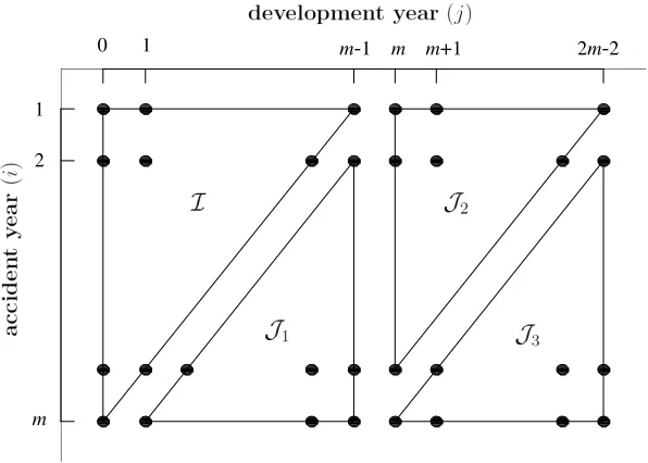
[image:13.595.129.427.252.465.2]The index sets I and J1 are illustrated in Figure 1.
Figure 1: Index sets for reserves.
The cash flow predicted by the chain ladder is shown in the last column of Table 6. The cash flow by calendar year is computed by summing the point forecasts ˜Xij along the diagonals of J1. Table 6 also shows the RBNS
general feature of the new method. Similar conclusions were noted in Verrall, Nielsen and Jessen (2010).
5.2
Point forecasts of the RBNS reserve
Forecasting the RBNS reserve by the cash flow model assumes that the pay-ments relating to the incurred counts are delayed as described in§3.1. These forecasts vary over the index set J1 as well as the index set
J2 ={i= 1, . . . , m;j =m, . . .2m−2 where i+j =m+ 1, . . . ,2m−1},
illustrated in Figure 1.
The point forecasts are constructed from the conditional expectation
mij(N) in (3). Recognising that the counts are only available in the
up-per triangle I and inserting the estimates ψℓb gives the point forecasts
˜
mij(N) =
min(j,d)
X
k=j−m+i
Ni,j−kψk,b (14)
over the index setJ1∪J2. The RBNS cash flow by calendar year is computed
by summing the point forecasts along the diagonals of J1∪ J2.
Point forecasts of the RBNS cash flow by calendar year for the motor data are shown in the first column of Table 6. Note that the cash flow for calendar year 19 is zero as the last delay parameter ψ9 is set to zero.
5.3
Point forecasts of the IBNR reserve
The IBNR forecasts are constructed in two stages. First, predictions of the incurred but not reported counts, ˜Nij are computed over the index set J1.
Secondly, these predictions are inserted in the expression ˜mij(N) to get the
IBNR point forecasts
˜
mij( ˜N) =
min(d,j−m+i−1)
X
k=max(0,j−m+1)
˜
Ni,j−kψk.b (15)
Due to the delay, these point forecasts run over the index sets J1,J2 as well
as the index set
illustrated in Figure 1.
The IBNR cash flow is shown in the last column of Table 6. The cash flow by calendar year is computed by summing the point forecasts along the diagonals of J1∪ J2 ∪ J3. As the last delay parameter ψ9 is set to zero the
cash flow for calendar year 28 is zero.
6
Bootstrapping the predictive distribution
including parameter uncertainty
In this section, we explain the bootstrapping procedure which can be applied to the model set out above. It should be noted that the term ’bootstrapping’ can be used to cover a wide range of approaches. For example, it is sometimes used in connection with procedures that just simulate the process distribu-tion. However, it is more common (especially in the actuarial literature) to use it when the estimation error is also included, and this is the context in which it is used in this paper. For completeness, we will also mention the former case in section 6.2, but all the results will include the estimation error. A further distinction in bootstrapping methodology is between parametric and non-parametric bootstrapping. Again, in the actuarial literature, it is more common to encounter non-parametric bootstrapping, where (for exam-ple) the residuals of the model are resampled. However, it is possible also to use parametric bootstrapping, and the choice may depend on the partic-ular properties of the model being considered. In the case of the model in this paper, parametric bootstrapping is more appropriate and is used in the remainder of this section. The results of this parametric bootstrapping esti-mation procedure are compared with non-parametric bootstrapping applied to the chain-ladder technique in section 6.3. In section 7, a simulation study compares the conditional bootstrapping method with the classical uncondi-tional chain ladder method.
6.1
The predictive distribution
We first introduce some notation for the predictive distributions of the RBNS and IBNR reserves, which will be estimated by bootstrapping.
The reported countsNij are indexed overI. Their distribution is denoted
NI(ω) and is Poisson distributed with mean given in terms of the population
The distribution of the aggregated claims Xij over I ∪ J1 ∪ J2 arising
from the incurred counts Nij is denotedXij(θ, N), where θ= (p, µ, σ2). This
distribution is constructed sequentially. Given the incurred counts, the paid counts Nijpaid are defined over the set I ∪ J1∪ J2 through the formula (1).
The individual claims distribution (or the severity distribution) is assumed to be a gamma distribution with mean µ and variance σ2. Therefore, the shape parameter is λ = µ2/σ2, the scale parameter is κ = σ2/µ, and the
density is
f(y) = 1
γ(λ)κλy
λ−1exp(−y/κ) fory >0.
Note that the possibility of zero claims is excluded, in contrast to assumption in Verrall, Nielsen and Jessen (2010). Given the count Nijpaid, the aggregate claims Xij are then gamma distributed with shape Nijpaidλ and scale κ.
The RBNS reserve is the sum overJ1∪ J2 of the aggregate claims arising
from the reported counts N, that is ˜mij(N) as given in (14).
The IBNR reserve arises from the incurred but not reported counts Nije
over the lower triangle J1. These are Poisson distributed distributed in a
similar way to the reported counts, and in accordance with the notation above, their distribution is denoted NJ1(ρ,Φ). The aggregated claims over
J1 ∪ J2 ∪ J3 arising from the predicted counts Ne, ˜mij( ˜N) as given in (15),
will then have a mixture distribution Xij{θ,NJ1(ω)}.
The total reserve is found by adding the RBNS and the IBNR reserves.
6.2
Bootstrap predictive distribution of RBNS and IBNR
cash flow
The predictive reserve distributions will be estimated using a parametric bootstrapping procedure. As mentioned above, the term ‘bootstrapping’ is sometimes used to describe the situation where the unknown parameters are simply replaced by the estimated parameters (ignoring the estimation uncertainty). This would give the bootstrap estimators
RBNS(θ, Nb ), IBNR{θ,b NJ
1(ωb)}, Total{θ, N,b NJ1(ωb)}. (16)
The more usual bootstrapping procedure, taking parameter uncertainty into account, is defined as follows.
The delay and severity parametersθ = (p, µ, σ2) are estimated using the
the chain ladder parametersωare estimated using the model for the reported counts N. For the bootstrap, this can be replicated by considering these two distributions varying independently in spaces Θ and Ω say. The conditional distribution given N of the estimators of the delay and severity parameters is denoted Dθ(θ∗;N) while the distribution of the estimators of the chain
ladder parameters is denoted Cω(ω∗). Hence the bootstrap distributions of
the reserves are the mixtures
RBNSmix(θ, N) =
Z
θ∗∈Θ
RBNS(θ∗, N)dDθ(θ∗;N), (17)
IBNRmix{θ,NJ
1(ω)}
=
Z
(θ∗,ω∗)∈(Θ,Ω)
IBNR{θ∗,NJ
1(ω ∗)}dC
ω(ω∗)dDθ(θ∗;N), (18)
Totalmix{θ, N,NJ
1(ω)}
=
Z
(θ∗,ω∗)∈(Θ,Ω)
Total{θ∗, N,NJ1(ω∗)}dCω(ω∗)dDθ(θ∗;N). (19)
These bootstrap distributions are evaluated at the estimated parameters giv-ing the bootstrap estimators
RBNSmix(θ, Nb ),IBNRmix{θ,bNJ
1(ωb)}, Totalmix{θ, N,b NJ1(ωb)}. (20)
As the integral (17), (18), (19) cannot be calculated exactly they are ap-proximated by simulation by drawing 999 repetitions of the independent distributionsCω(ω∗)D
θ(θ∗;N). In each repetition the integrand is evaluated
as in (16).
To implement the above bootstrap approximations we define the following bootstrap algorithms for the RBNS and IBNR cash-flows.
Algorithm RBNS
Step 1. Estimation of the parameters and distributions. From the original data (N,X) estimate the parameters in the model byθb= (p,b µ,b σb2) through
(10) and (8). The delay distribution is estimated by a multinomial dis-tribution with probability parameterpb. The distribution of the individ-ual payments is estimated by a gamma with shape parameterbλ=µb2/
b σ2
and scale parameter bκ=bσ2/
b µ.
Step 2. Bootstrapping the data. Keep the same counts N but generate new bootstrapped aggregated paymentsX∗ ={X∗
• Simulate the delay: from eachNij inIgenerate the number of paid claims,Nij∗paid, by (1) from the Multinomial distribution estimated at Step 1.
• Get the bootstrapped aggregated payments, X∗
ij, from a gamma
distribution with shape parameterNij∗paidλband scale parameterbκ, for each (i, j)∈ I.
Step 3. Bootstrapping the parameters. From the bootstrap data, (N, X∗), get
θ∗ = (p∗, µ∗, σ2∗), calculated in the same way as θbbut with the
boot-strap data generated at Step 2.
Step 4. Bootstrapping the RBNS predictions.
• Simulate the delay from the Multinomial distribution with boot-strapped probability parameter p∗ (as in Step 2). Calculate the
number of RBNS claims trough (1) and denote these values by
N∗rbns
ij , with (i, j)∈ J1∪ J2.
• Get the bootstrapped RBNS predictions, m∗
ij(N), from a gamma
distribution with shape parameter N∗rbns
ij λ∗ and scale parameter κ∗. Here λ∗ =µ∗2/σ2∗ and κ∗ =σ2∗/µ∗.
Step 5. Monte Carlo approximation. Repeat steps 2-4 B times and get the empirical bootstrap distribution of the RBNS reserve, mije (N), from the bootstrapped {m∗ij(b)(N), b= 1, . . . , B}, for each (i, j)∈ J1∪ J2.
Algorithm IBNR
Step 1. Estimation of the parameters and distributions. Estimate θ as in Step 1 of Algorithm RBNS, above. Estimate ω using chain ladder, through (5) and (6).
Step 2. Bootstrapping the data. Get new bootstrapped data (N∗, X∗) as
fol-lows:
• The countsN∗are simulated from Poisson distributions with mean
• The bootstrapped aggregated paymentsX∗ are simulated exactly
as was described in Step 2 of the algorithm RBNS above.
Step 3. Bootstrapping the parameters. From the bootstrap data, (N, X∗), get θ∗ = (π∗, µ∗, σ2∗), and ω∗ = (ρ∗,Φ∗) calculated in the same way as
(θ,b bω), but with the bootstrapped data generated at Step 2. Calculate the bootstrapped count parameters, ω∗, by (5) using N∗, and get the
bootstrapped predictions in the lower triangle N∗ J1(ω
∗).
Step 4. Bootstrapping the IBNR predictions.
• For each entry N∗
ij in NJ∗1(ω
∗), simulate the delay from a
Multi-nomial distribution with bootstrapped probability parameter p∗.
Calculate the number of IBNR claims trough (1) and denote these values byN∗ibnr
ij , for each (i, j)∈ J1∪ J2∪ J3.
• Get the bootstrapped IBNR predictions, m∗ij(NJ1∗ (ω∗)), from a
gamma distribution with shape parameter N∗ibnr
ij λ∗ and scale
pa-rameterκ∗, exactly as in algorithm RBNS.
Step 5. Monte Carlo approximation. Repeat steps 2-4 B times and get the empirical bootstrap distribution of the IBNR reserve,mije (N), from the bootstrapped {m∗ij(b)(N), b = 1, . . . , B}, for each (i, j)∈ J1∪ J2∪ J3.
An intuitive representation of the above bootstrap algorithms are given in Figures 2 and 3.
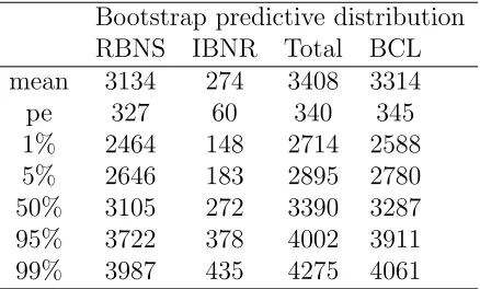
Considering the motor data, the summary statistics from the RBNS and IBNR cash-flows, estimated by the just presented bootstrap method are re-ported in Table 7.
6.3
A comparison with bootstrap estimation for the
chain ladder technique
Figure 2: Bootstrapping scheme to approximate the RBNS predictive distri-bution
necessary to ensure that these residuals are independent and identically dis-tributed. This contrasts with the bootstrap method described above, which is a parametric bootstrap exploiting an assumed distributional form and defining the resampling scheme from the parametric distributions. Other parametric bootstrap methods have been considered recently by Bj¨orkwall, H¨ossjer and Ohlsson (2009a, 2009b).
for the chain ladder method. Again, we note that the new model includes the tail and we would expect that the prediction error for the chain ladder model would increase once this is taken into account. Also shown are some percentiles of the bootstrap estimates of the predicitive distributions for the new model and the chain ladder model. In order to assess the performance of the new model, the following section contains a simulation study to compare the results with the classical chain ladder.
7
Simulation study
In order to study the performance of the model described in this paper, in comparison with the standard chain ladder technique, this section considers a simulation study and examines the reserve estimates and capital requirements based on each approach. We generate the data using the assumptions of the new model, but (since the assumptions are deliberately free of any specific structure in terms of the shape of the run-off) we do not believe that this has any affect on the conclusions reached.
7.1
The simulation settings
A scenario for the simulations close to that described in section 6 has been constructed. We consider data triangles with dimensionk= 10, and generate 999 data sets using the following distribution specifications:
1. The reported countsNij are defined over a square matrix (with dimen-sion m = 10) with the upper triangle being exactly the data entries in Table 1, and the lower triangle completed by generating the entries from a Poisson model with the chain ladder parameters.
2. The delay is generated from a multinomial distribution with probability parameters pk estimated from the empirical study in section 5.
3. The individual payments are generated from a gamma distribution with first two moments, µ = 163.6158 and σ2 = 2070821 (estimated again
from the empirical study).
7.2
Distribution forecasts
We study the performance of the new bootstrap method (described through algorithms in Section 6.2) in estimating the predictive distribution. Also we make comparisons with the results achieved by applying the standard bootstrap method to the chain ladder method. As in the empirical study in Section 6, we fix the number of bootstrap samples to be B = 999 for all the bootstrap methods.
In order to assess the performance of the new method, we require the ”actual” predictive distribution, which we simulate using steps 1–4 of the simulations described above. This was done as follows: for each of the 999 simulated data sets we estimate the parameters in the model. These esti-mates are used to produce the RBNS and IBNR reserves, and from these 999 reserves we calculate the desired quantile of the distribution. This process is repeated 999 times and the simulated ”actual” quantiles are defined as by taking the average of the 999 resulting quantiles.
Table 8 shows the distribution forecasts for the total reserve. The boot-strap chain ladder method of England and Verrall (2002) and England (2002), as implemented by Gesmann (2009) gives higher tail quantiles implying higher levels of solvency requirements when using this method. One can consider the trade-off between accepting these extra solvency requirements based on the simple unconditional chain ladder method and rather than collecting the triangle data of reported claims and implementing the more complicated model considered in this paper.
predicted.
8
Conclusions
This paper has examined the properties of the claims reserving method pro-posed by Verrall, Nielsen and Jessen (2010), and has shown how the full predictive distribution may be obtained using bootstrap methods. In this paper, the structure of the model is identical to Verrall, Nielsen and Jessen (2010) although the detailed assumptions differ in some respects. We believe that this general approach has a great deal to offer: it is essentially as simple to apply as methods such as the chain-ladder technique, but it uses a little more data. We believe that by adding the information regarding the claim counts, much better estimates should be obtained (in general) for the out-standing liabilities and for the predictive distributions. Although the results for the set of data used in this paper did not show any great improvements over the standard chain ladder results, we believe that the general approach has a lot of potential for further development and improvement. We also believe that the coherent approach to the underlying mechanism generating the data, the split between RBNS and IBNR reserves, and the natural and consistent inclusion of the tail in the forecasts are specific advantages of this methods over the ad hoc approach of the chain ladder technique.
Acknowledgement
The computations were done using R (R Development Core Team, 2006). This research was financially supported by a Cass Business School Pump Priming Grant. The first author is also supported by the Project MTM2008-03010/MTM.
References
Bj¨orkwall, S., H¨ossjer, O. & Ohlsson, E. (2009b) Bootstrapping the separa-tion method in claims reserving. Stockholm University, Mathematical Statistics, Research Report 2009:2. To appear in ASTIN Bulletin
Bryden, D. and Verrall, R.J. (2009) Calendar year effects, claims inflaton and the Chain-Ladder technique. Annals of Actuarial Science 4, 287-301.
England, P. (2002) Addendum to “Analytic and Bootstrap Estimates of Prediction Error in Claims Reserving”. Insurance: Mathematics and Economics 31, 461–466.
England, P. & Verrall, R. (1999) Analytic and Bootstrap Estimates of Pre-diction Error in Claims Reserving. Insurance: Mathematics and Eco-nomics 25, 281–293.
Gesmann, M. (2009) R-package ‘ChainLadder’ version 0.1.2-11 (April, 17, 2009).
Kremer, E. (1985)Einf¨uhrung in die Versicherungsmathematik. G¨ottingen: Vandenhoek & Ruprecht.
Kuang, D., Nielsen, B. & Nielsen, J.P. (2008a) Identification of the age-period-cohort model and the extended chain-ladder model. Biometrika
95, 979–986.
Kuang, D., Nielsen, B. & Nielsen, J.P. (2008b) Forecasting with the age-period-cohort model and the extended chain-ladder model. Biometrika
95, 987–991.
Kuang, D., Nielsen, B. & Nielsen, J.P. (2009) Chain Ladder as Maximum Likelihood Revisited. Annals of Actuarial Science 4, 105–121.
Kuang, D., Nielsen, B. & Nielsen, J.P. (2010) Forecasting in an extended chain-ladder-type model. Journal of Risk and Insurance to appear.
Mack, T. (1991) A simple parametric model for rating automobile insurance or estimating IBNR claims reserves. Astin Bulletin, vol. 39, 35–60.
R Development Core Team (2006). R: A Language and Environment
for Statistical Computing. Vienna: R Foundation for Statistical Com-puting.
Taylor, G. (1977) Separation of inflation and other effects from the distri-bution of non-life insurance claim delays. ASTIN Bulletin 9, 217–230.
Verrall, R., Nielsen, J.P. & Jessen, A. (2010) Prediction of RBNS and IBNR claims using claim amounts and claim counts. To appear in ASTIN Bulletin.
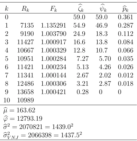
k Rk Fk ζkb ψkb pkb
0 59.0 59.0 0.361 1 7135 1.135291 54.9 46.9 0.287 2 9190 1.003790 24.9 18.3 0.112 3 11427 1.000917 16.6 13.8 0.084 4 10667 1.000329 12.8 10.7 0.066 5 10951 1.000284 7.27 5.70 0.035 6 11421 1.000234 5.13 4.26 0.026 7 11341 1.000144 2.67 2.02 0.012 8 12486 1.000306 3.21 2.87 0.018 9 13658 1.000421 0.28 0 0 10 10989
b
µ= 163.62
b
ϕ= 12793.19
b
σ2 = 2070821 = 1439.02
b σ2
[image:27.595.187.424.229.474.2]V N J = 2066398 = 1437.52
Table 5: Estimates for motor data. RkandFk are row sums and development factors for count data in Table 1 computed as in (5). ψkb , pkb , µb are delay parameters estimated as described in §4.2 using the analytic method with a negative ψb9 replaced by zero. ϕb and bσ2 are computed as in (12), (13).
b σ2
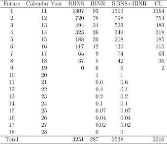
Future Calendar Year RBNS IBNR RBNS+IBNR CL
1 11 1307 93 1399 1354
2 12 720 78 798 754
3 13 494 34 529 489
4 14 323 26 349 318
5 15 188 20 208 185
6 16 117 12 130 115
7 17 65 9 74 63
8 18 37 5 42 36
9 19 0 6 6 2
10 20 1 1
11 21 0.6 0.6
12 22 0.4 0.4
13 23 0.2 0.2
14 24 0.1 0.1
15 25 0.07 0.07
16 26 0.04 0.04
17 27 0.02 0.02
18 28 0 0
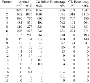
[image:28.595.135.474.236.528.2]Total 3251 287 3538 3316
Bootstrap predictive distribution RBNS IBNR Total BCL mean 3134 274 3408 3314 pe 327 60 340 345 1% 2464 148 2714 2588 5% 2646 183 2895 2780 50% 3105 272 3390 3287 95% 3722 378 4002 3911 99% 3987 435 4275 4061
Future Actual Cashflow Bootstrap CL Bootstrap 95% 99% 95% 99% 95% 99% 1 1649 1759 1659 1776 1709 1847 2 992 1085 1001 1094 1018 1115 3 686 765 698 778 707 789 4 482 550 492 562 494 564 5 319 375 326 386 323 381 6 226 276 231 284 224 274 7 157 203 161 210 150 193 8 112 154 117 163 103 140
9 41 76 48 87 24 41
10 9 23 10 25 0 0
11 3 14 3 13 0 0
12 0.8 10 1.4 9 0 0
13 0.2 7 0.4 5 0 0
14 0 3 0.1 3 0 0
15 0 0.8 0 1 0 0
16 0 0.1 0 0.4 0 0
17 0 0 0 0.1 0 0
[image:30.595.146.458.216.506.2]18 0 0 0 0 0 0
Future Actual Cashflow Bootstrap CL Bootstrap
1 1396 1406 1400
2 793 802 799
3 523 530 528
4 343 350 345
5 203 209 204
6 124 129 124
7 69 74 68
8 38 42 36
9 4 7 3
10 0 0 0
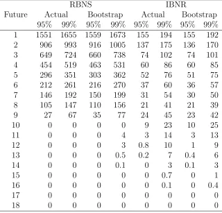
RBNS IBNR
Future Actual Bootstrap Actual Bootstrap 95% 99% 95% 99% 95% 99% 95% 99% 1 1551 1655 1559 1673 155 194 155 192 2 906 993 916 1005 137 175 136 170 3 649 724 660 738 74 102 74 101 4 454 519 463 531 60 86 60 85 5 296 351 303 362 52 76 51 75 6 212 261 216 270 37 60 36 57 7 146 192 150 199 31 54 30 50 8 105 147 110 156 21 41 21 39 9 27 67 35 77 24 45 23 42
10 0 0 0 0 9 23 10 25
11 0 0 0 4 3 14 3 13
12 0 0 0 3 0.8 10 1 9
13 0 0 0 0.5 0.2 7 0.4 6 14 0 0 0 0.1 0 3 0.1 3
15 0 0 0 0 0 0.7 0 1
16 0 0 0 0 0 0.1 0 0.4
17 0 0 0 0 0 0 0 0
[image:32.595.143.463.207.514.2]18 0 0 0 0 0 0 0 0