An improved convolution algorithm for discretely sampled Asian options

City, University of London Institutional Repository

Citation

:

Černý, A. & Kyriakou, I. (2010). An improved convolution algorithm for discretely sampled Asian options. Quantitative Finance, 11(3), pp. 381-389. doi:

10.1080/14697680903397667

This is the accepted version of the paper.

This version of the publication may differ from the final published

version.

Permanent repository link:

http://openaccess.city.ac.uk/12180/

Link to published version

:

http://dx.doi.org/10.1080/14697680903397667

Copyright and reuse:

City Research Online aims to make research

outputs of City, University of London available to a wider audience.

Copyright and Moral Rights remain with the author(s) and/or copyright

holders. URLs from City Research Online may be freely distributed and

linked to.

City Research Online: http://openaccess.city.ac.uk/ [email protected]

Electronic copy available at: http://ssrn.com/abstract=1323252 Electronic copy available at: http://ssrn.com/abstract=1323252

DISCRETELY SAMPLED ASIAN OPTIONS

ALEŠ µCERNÝ AND IOANNIS KYRIAKOU

Abstract. We suggest an improved FFT pricing algorithm for dis-cretely sampled Asian options with general independently distributed re-turns in the underlying. Our work complements the studies of Carverhill and Clewlow (1990), Benhamou (2002), and Fusai and Meucci (2008), and, if we restrict our attention only to lognormally distributed returns, also Veµceµr (2002). While the existing convolution algorithms compute the density of the underlying state variable by moving forward on a suitably de…ned state space grid our new algorithm usesbackward price convolution, which resembles classical lattice pricing algorithms. For the …rst time in the literature we provide an analytical upper bound for the pricing error caused by the truncation of the state space grid and by the curtailment of the integration range. We highlight the bene…ts of the new scheme and benchmark its performance against existing …nite di¤erence, Monte Carlo, and forward density convolution algorithms.

1. Introduction

Asian options represent a class of derivative securities whose payo¤ de-pends on an average price of the underlying asset during a prespeci…ed time window. Their appeal stems partly from the fact that average price is harder to manipulate by unscrupulous traders and partly because the averaging re-duces the volatility of the underlying asset and thus leads to lower option prices.

The manner of averaging has a signi…cant impact on the analytical tracta-bility of Asian options. The literature distinguishes geometric versus arith-metic averaging and continuous versus discrete sampling of the underlying price. While the geometric average admits a closed-form solution in the

Date: October 8, 2009.

1991 Mathematics Subject Classi…cation. Primary 91B28; Secondary 60H05, 60J60, 93E20.

Key words and phrases. Asian options, discrete sampling, convolution, FFT.

We would like to thank Gianluca Fusai and Jan Veµceµr for helpful discussions. We are also grateful to two anonymous referees for helpful comments and suggestions. The work of Ioannis Kyriakou was supported by the Cass Business School Doctoral Programme and the EPSRC.

Electronic copy available at: http://ssrn.com/abstract=1323252 Electronic copy available at: http://ssrn.com/abstract=1323252

Black-Scholes model (cf. Turnbull and Wakeman 1991), for the more preva-lent arithmetic average no simple analytical solution exists1_{. The Asian case} is complicated by the fact that one wishes to achieve a reduction in the number of state variables. This reduction, foreshadowed in Ingersoll (1987) and employed in Rogers and Shi (1995), Andreasen (1998), Veµceµr (2001) and Veµceµr (2002), uses a change of measure and requires the option pay-o¤ to be a homogeneous function of the weighted average of stock prices. The same applies to the PIDE of Veµceµr and Xu (2004) which is implemented numeri-cally for continuously monitored Asians under jump-di¤usions in Bayraktar and Xing (2008).

Most Asian options are not sampled continuously, indeed it is typical for the underlying price to be recorded only once a day or once a week. The above PDE techniques2 _{can be modi…ed to accommodate discrete sampling} (cf. Andreasen 1998, Veµceµr 2002), but they do not exploit discrete sam-pling to their advantage. If anything, discrete samsam-pling has a detrimental e¤ect on the …nite di¤erence algorithms by making the PDE coe¢ cients dis-continuous and therefore eroding the quadratic convergence in time of the Crank-Nicolson scheme.

There are three existing papers, Carverhill and Clewlow (1990), Ben-hamou (2002) and Fusai and Meucci (2008), which are speci…cally tailored to discretely sampled Asians while simultaneously exploiting a state space reduction similar to the one mentioned above, using so-called Carverhill-Clewlow-Hodges factorization. In all three papers the computation works by evaluating the density of the average price goingforward. These papers have a signi…cant advantage over the PDE techniques in that they are easily extended to allow for leptokurtic returns in the underlying without being restricted to jump-di¤usions.

By exploiting the notion of a reverse …ltration we are able to replace the Carverhill-Clewlow forward density convolution by a backward price con-volution. We demonstrate below that this has substantial numerical and theoretical advantages. The paper is organized as follows: In Section 2 we introduce the notation and the Carverhill-Clewlow-Hodges factorization. In Section 3 we develop the main theoretical results for the backward price

1_{See Linetsky (2004) and references therein for transform methods and their numerical} implementation.

convolution scheme, and in Section 4 we discuss its implementation via dis-crete Fourier transform. In Section 5 we describe parametrization of log return distribution for the Black-Scholes model and two Lévy process mod-els, the tempered stable and normal inverse Gaussian. Section 6 concludes by comparing the speed and accuracy of our scheme with previous studies.

2. Preliminaries

Fix n_2N, and let _fZkgnk=1 be a collection of independent random vari-ables on the probability space _f ;_F; P_gsuch that 0 <Var(exp(Zk))<1.

Let _F := _fFkgn_k=1 be the information …ltration generated by the random

variables _fZkg, with F0 trivial. Fix a constant S0 >0 and de…ne the price process of a risky asset

Sj :=S0exp(

j

X

k=1

Zk); j = 1; : : : ; n;

and a risk-free bank account with total return Rk in periodk2 f1; : : : ; ng.

We assume period kdividend payment of the size (Dk 1)Sk 1; Dk 1.

We interpret P as a risk-neutral measure. In the presence of dividends we therefore have

E(eZk_{) =R}

k=Dk:= k fork= 1; : : : ; n:

The collection _fZkgnk=1 is completely general at this stage. In speci…c ap-plications one may allow Zk-s to follow a non-parametric distribution or

identify them with increments of a speci…c Lévy process (see Section 5). In the Black–Scholes model with sampling dates t1; : : : ; tn one has

Zk N((r 2=2)(tk tk 1); 2(tk tk 1));

Rk = exp(r(tk tk 1));

Dk = exp(^(tk tk 1));

where represents the volatility of log returns, r is the risk-free rate and^ the dividend yield.

Fix a deterministic process and de…ne a process of partial sums

Ij := j

X

k=0

kSk: (2.1)

Pricing of …xed or ‡oating strike call/put options amounts to calculating

E(I_n+); (2.2)

Option type 0 1; : : : ; n 1 n

Call, …xed strike _{n+ S}K

0

1

n+

1

n+ Call, ‡oating strike _{n+ n+} 1 _n+ Put, …xed strike _SK

0 n+

1

n+

1

[image:5.612.146.460.104.217.2]

n+ Put, ‡oating strike _{n+ n+ n+} 1

Table 1. Choice of corresponding to di¤erent types of Asian options. >0 is the coe¢ cient of partiality for ‡oat-ing strike options. Coe¢ cient takes value 1 (0) whenS0 is (is not) included in the average.

The computational di¢ culty stems from the fact that I is not a Markov process underP. More speci…callySis Markov and(S; I)are jointly Markov underPwhich means, when evaluating (2.2) recursively, that the conditional expectationE(I+

njFt)depends on both Stand It:This implies pricing must

be performed on a 3-dimensional grid(I; S;time). Let us now de…ne a new …ltration_G:=_fGigni=1

Gi = fZn; Zn 1; : : : ; Zn i+1g; and process X by setting

Xk := n k+Xk 1exp(Zn+1 k); (2.3)

X0 := n:

We can now state a generalized version of the Carverhill-Clewlow-Hodges factorization3.

Proposition 2.1. Consider deterministic coe¢ cients_f kgnk=0and processes

I; X de…ned in (2.1), (2.3). The following statements hold:

(1) The random variables In; Xn satisfy

In=S0Xn; (2.4)

(2) Process X is Markov in …ltration _G under measure P.

Proof. (1) follows by recursive substitution. (2) follows from the stochastic independence of variables _fZkgn_k=1:

3_{We do not require to be constant or of the same sign and we do not need variables}

3. Backward price convolution algorithm

Proposition 2.1 signi…es that one can price the Asian option by evaluating

S0E(Xn+) recursively in …ltration G. Now assume that i 0 for i =

1; : : : ; n: This, by virtue of (2.3), implies Xk >0 for0 k < n and in turn

we obtain

Xk n k >0 for1 k < n:

Thus we can write (2.3) alternatively as

ln(Xk n k) = lnXk 1+Zn+1 k: (3.1)

Carverhill and Clewlow (1990), Benhamou (2002) and Fusai and Meucci (2008) use this transition equation to compute the unconditional risk-neutral density of ln(Xn 0) which they subsequently use to price a …xed strike

Asian call option. This is done recursively, evaluating the density ofln(Xk n k) as the convolution of densities of lnXk 1 and Zn+1 k in line with

equation (3.1). In the …rst two papers the convolution is computed by Fourier transform, in the third paper it is computed directly.

In all three papers the di¢ culty is that the density of ln(Xk n k)

spreads out as k increases. This problem is not speci…c to Asian options, the same situation would occur if one applied the density method iteratively to plain vanilla options in the Black-Scholes model. Ideally, one should use a dense and narrow grid for ln(X1 n 1) and wide and relatively sparse grid for ln(Xn 0). Clewlow and Carverhill use the same equidistantly spaced grid for all variables ln(Xk n k): Benhamou (2002) models

re-centered variables ln(Xk n k) on a common grid. Fusai and Meucci

(2008) use a …xed grid that is not equidistant to take advantage of Gaussian numerical integration. Simultaneous recentering and rescaling has not been implemented in the literature, to the best of our knowledge, although the methodology of Fusai and Meucci (2008) allows this in principle.

Theorem 3.1. Assume that for allk the CDF of Zn+1 k has a density fk

with respect to the Lebesgue measure on _R, satisfying

k:=

Z

R

ezfk(z)dz <1:

Consider constants k > 0;0 < k n and 0 2 R. De…ne functions

pk:R!R for 0< k n and qk; hk:R!R for 0 k < n as follows

pn(y) := (ey+ 0)+;

hk(y) := ln(ey+ n k);0< k < n;

qk 1(x) :=

Z

R

pk(x+z)fk(z)dz;0< k n; (3.2)

pk 1(y) := qk 1(hk 1(y));1< k n: (3.3)

The following statements hold:

(1) The forward price of an Asian call contract with parameters _f jgn_j=0

is given by

E(I_n+) =S0E(Xn+) =S0q0(ln n):

(2) There are positive constants ak; bk such that for all x; y2R

0 pk(y) akey+bk; (3.4)

0 qk(x) akex+bk+1: (3.5)

These constants are given recursively by

an = 1; bn= +0; (3.6)

ak 1 = ak k; (3.7)

bk 1 = bk+ak 1 n k+1: (3.8) In numerical applications we must curtail the range of integration in (3.2). In the next theorem we estimate the pricing error caused by the curtailment and provide a constructive method for …nding the curtailed ranges.

Theorem 3.2. Consider the following (exponential) tail moments

Fk(z; ) =

Z z

1

e xfk(x)dx;

Gk(z; ) =

Z ₁

z

e xfk(x)dx:

Under the assumptions of Theorem 3.1 Fk(z; 1) +Gk(z; 1) = k and

lim

Consider compact intervals_f[lk; uk]gn_k=1and de…ne compact intervalsf[Lk; Uk]gn_k=1;

f[Lk; Uk]gnk=01 by setting

L0 = U0= ln n; (3.9)

Lk = Lk 1+lk; Uk=Uk 1+uk;0< k n; (3.10)

Lk = ln(eLk+ n k); Uk= ln(eUk+ n k);0< k < n: (3.11)

De…ne functions q~k;p~k by setting

~

qk 1(x) := ( Z

R

~

pk(x+z)fk(z)dz)1[Lk 1;Uk 1](x);0< k n;

~

pk 1(y) := q~k 1(hk 1(y))1[Lk 1;Uk 1](y);1< k n;

~

pn(y) := pn(y)1[Ln;Un](y)

Let ~an= ~bn= 0 and for 0< k n recursively de…ne

~

ak 1 = a~k k+ak(Fk(lk; 1) +Gk(uk; 1));

~_{bk 1 = a~k 1 n k+1+ ~bk+bk(Fk(lk; 0) +Gk(lk; 0));}

where ak; bk are given by (3.6-3.8).

(1) The pricing error has the following bounds

0 q0(ln n) q~0(ln n) ~b0; (3.12)

and~b0>0can be made arbitrarily small by suitable choice off[lk; uk]gnk=1: (2) For k < n and positive constants ck de…ned recursively by cn =

0; ck 1=ck+ak 1 n k+1 we have

0 p~0_k(y) akey+ck for y2(Lk; Uk); (3.13)

0 q~_k0(x) ak 1ex+ck for x2(Lk; Uk) (3.14)

(3) Functions_fp~kgn_k=11;fq~kgn_k=01 are continuously di¤ erentiable on the

in-terior of their support.

(4) For 0 k < n andx₂(Lk; Uk)

~

qk 1(x) =F 1(F(~pk) k)(x); (3.15)

where _F denotes the Fourier transform (see Appendix A), _k is the characteristic function of Zn k

k(u) :=

Z

R

eiuzfk(z)dz;

and _k denotes its complex conjugate.

principle is used in Lord et al. (2008) for the computation of the delta and gamma of a European plain vanilla option, and more generally in the case of Bermudan options with multiple exercise dates. Using this method the computational e¤ort for sensitivities is of the same order as computational e¤ort for prices.

4. Numerical implementation

De…nition 4.1. Consider two uniform grids x =_fx0+j xgnj=01 and u =

fu0+k ugm_k=01 and vector a = fajgnj=01. We de…ne a generalized discrete

Fourier transform (DFT) of a from x onto u as the m-dimensional vector

b=_fbkgmk=01 satisfying

bk= n 1 X

j=0

ajeixjuk = n 1 X

j=0

ajei(x0+j x)(u0+k u):

We write b=_D(a;x;u):

This is a very slight generalization of transforms that feature prominently in the signal processing literature. When x0 =u0 = 0 we obtain so-called fractional Fourier transform with fractionality coe¢ cient = n x u₂ . When furthermore m =n and = 1 we obtain the standard DFT. In this paper we compute the generalized DFT by means of so-called chirp z-transform4 (CZT), which is readily available in MATLAB.

De…nition 4.2. Consider vector a = _fajg_jn₌₀1, and parameters m 2 N,

A; w_2C:The chirpz-transform of a with parameters A; w; m is the vector

b=_fbkgm_k=01 satisfying

bk= n_X1

j=0

aj(Aw k)j:

We write b= czt(a; A; w; m):

Proposition 4.3. Consider two uniform grids x=_fx0+j xgnj=01 andu=

fu0+k ugm_k=01 and vector a=fajgnj=01. We have

D(a;x;u) =eix0u_{czt(a; e}iu0 x_{; e} i x u_{; m): (4.1)}

Proof. Straightforward algebra.

Our numerical algorithm proceeds as follows:

4_{CZT pre-dates FrFT by more than 20 years, see Rabiner et al. (1969). It is more}

(1) For a given contract we …nd values of lk; uk that achieve a

prede-termined pricing precision given by (3.12). We evaluate the tail moments by Fourier inversion

Fk(x; ) =

1 2 clim!1

Z c

c

k(u i( + ))

iu+ e

(iu+ )x_du;

Gk(x; ) =

1 2 clim!1

Z c

c

k(u i( + ))

iu+ e

(iu+ )x_du;

for suitably chosen constants <0; >0(cf. Strawderman 2004). (2) We then determine the grid ranges[Lk; Uk]and[Lk; Uk]for functions

~

pk;q~k via (3.9-3.11).

(3) We select a uniform grid u symmetric around zero. The range of values in u is determined to ensure _{j kj}< outside u. The value of is guided by the desired precision, i.e. we pick = 10 7 when computing results to 7 decimal places.

(4) Suppose the values approximating p~k are given on a uniform grid y

and the values of _k are given on a uniform grid u. By abuse of notation we denote the function values on the grid by p~k and k,

respectively. We evaluate Pk := D(~pk;y;u) as a discrete

approx-imation of the transform _F(~pk): We then approximate the inverse

Fourier transform (3.15) by computing q~k 1 = D(Pk₂k; u;x) where

x is a uniform grid on the interval [Lk 1; Uk 1]. The generalized DFT is implemented via fast CZT using the conversion (4.1). (5) We approximate q~k 1 inside grid x by a cubic interpolating spline

…tted to the nodes (x;~qk 1) using not-a-knot endpoint conditions. Outside xwe approximate q~k 1 by extrapolating linearly in ex. We compute ~pk 1 = ~qk 1(hk 1(y))and continue with item 4.

Theoretically we expect quadratic convergence of the price as a function of the grid spacing for gridsx;y;u. Let nbe a numerical price corresponding

to multiplier 2 n of the original spacing on grids x;y;u. We expect n n+1 4( n+1 n+2)and we indeed observe n n+1 = (4 10 2)( n+1

n+2) for n su¢ ciently high. At this point if two consecutive Richardson

extrapolations agree to the desired precision we terminate the algorithm. We then increase grid range foru and run the whole computation again to con…rm that the results agree to the desired number of decimal places.

5. Leptokurtic stock returns

underlying Lévy process by L the risk-neutral characteristic function is given by the formula

E(eiuLt_{) = e}^(iu)t_{; (5.1)} ^(u) = (u) +u(r ^ (1));

where t is the time horizon measured in years and ^ is the dividend yield. The cumulant generating functions (u) for the di¤erent models are given as follows,

G(u) = 2u2=2;

CGMY(u) = C ( Y) ((M u)Y MY + (G+u)Y GY); NIG(u) = (1

p

1 2 u 2_u2_{)= :}

By a standard result (cf. Cont and Tankov 2004, Section 2.2.5)Lhas the following unconditional moments

E(Lt) = ^0(0)t= ( 0(0) +r ^ (1))t;

Var(Lt) = ^00(0)t= 00(0)t;

skew(Lt) =

^000(0) (^00(0))3=2t

1=2₌ 000(0) ( 00₍₀₎₎3=2t

1=2_;

kurt(Lt) = 3 +

^(4)(0) (^00(0))2t

1_{= 3 +} (4)(0) ( 00₍₀₎₎2t

1_:

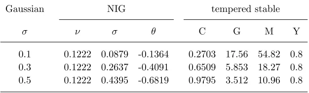
We calibrate the three models to achievepVar(L1)2 f0:1;0:3;0:5gand for the non-Gaussian distributions we further require

skew(L1) = 0:5; (5.2) kurt(L1) = 3:7: (5.3)

These moments are broadly consistent with risk-neutral densities …tted to option price data by Madan et al. (1998) and Carr et al. (2002). The …tted parameters, rounded to four leading digits, are summarized in Table 2.

Gaussian NIG tempered stable

C G M Y

[image:11.612.150.463.559.653.2]

0.1 0.1222 0.0879 -0.1364 0.2703 17.56 54.82 0.8 0.3 0.1222 0.2637 -0.4091 0.6509 5.853 18.27 0.8 0.5 0.1222 0.4395 -0.6819 0.9795 3.512 10.96 0.8

6. Numerical results

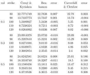
6.1. Black-Scholes model. Our algorithm is a major improvement over existing density convolution pricing procedures. In Table 3 we present our results with precision 10 7; alongside the original numbers of Carverhill and Clewlow (1990) and Benhamou (2002). We observe that the original results are at best precise to 3 decimal places, but often not even to 2 decimal places. The precision is better for low volatilities.

vol strike Cerný &µ Ben- error Carverhill error Kyriakou hamou & Clewlow

80 22.7771749 22.7838 0.007 22.78 0.003 90 13.7337773 13.7347 0.001 13.73 -0.004 0.1 100 5.2489927 5.2438 -0.005 5.25 0.001

110 0.7238324 0.7211 -0.003 0.72 -0.004 120 0.0264092 0.0336 0.007 0.02 -0.006

80 23.0914378 23.0733 -0.018 23.09 -0.001 90 15.2207610 15.2231 0.002 15.29 0.069 0.3 100 9.0271888 9.0110 -0.016 9.08 0.053 110 4.8349071 4.8338 -0.001 4.86 0.025 120 2.3682854 2.3545 -0.014 2.4 0.032

[image:12.612.155.460.232.485.2]

80 24.8242581 24.8324 0.008 25.01 0.186 90 18.3316740 18.3207 -0.011 18.5 0.168 0.5 100 13.1580456 13.1811 0.023 13.47 0.312 110 9.2345134 9.2300 -0.005 9.45 0.215 120 6.3719536 6.3615 -0.010 6.68 0.308

Table 3. Comparison with Benhamou (2002) and Carverhill and Clewlow (1990) for lognormal returns. Asian call option parameters T = 1; n= 50; S0 = 100.

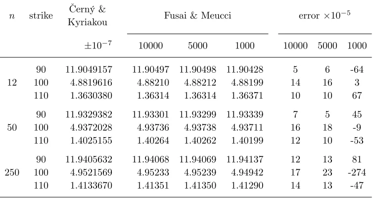
error for 10000 points in further four cases. This makes it hard for users of the density convolution method to gauge the precision of their scheme. Correspondingly, one can see that the results in Fusai and Meucci can be substantially less precise than the reported 5 decimal places.

n strike Cerný &µ

Kyriakou Fusai & Meucci error 10

5

10 7 _{10000 5000 1000 10000 5000 1000}

90 11.9049157 11.90497 11.90498 11.90428 5 6 -64 12 100 4.8819616 4.88210 4.88212 4.88199 14 16 3

110 1.3630380 1.36314 1.36314 1.36371 10 10 67

90 11.9329382 11.93301 11.93299 11.93339 7 5 45 50 100 4.9372028 4.93736 4.93738 4.93711 16 18 -9 110 1.4025155 1.40264 1.40262 1.40199 12 10 -53

90 11.9405632 11.94068 11.94069 11.94137 12 13 81 250 100 4.9521569 4.95233 4.95239 4.94942 17 23 -274

[image:13.612.127.504.194.395.2]

110 1.4133670 1.41351 1.41350 1.41290 14 13 -47

Table 4. Comparison with Fusai and Meucci (2008) for lognormal returns. Parameters T = 1; = 0:17801; r = 0:0367; n = 50; S0 = 100. Numbers 1000, 5000, 10000 in the last 6 columns signify the number of grid points used by Fusai and Meucci.

The execution time is in our favour since our control variate Monte Carlo takes longer than that of Fusai and Meucci (for n = 50 F&M need 130 seconds to run 1,000,000 MC trials while we need 190 seconds) but our pricing procedure is substantially faster (we need under 1 second to achieve guaranteed 5 decimal place precision while F&M require 5 seconds with 1000 quadrature points to achieve a variable precision of 3-4 decimal places; see our timings in Table 7).

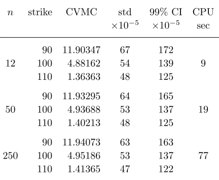
accuracy (at 99% con…dence level) while our method needs under 1 second to obtain 5 decimal places.

n strike CVMC std 99% CI CPU

10 5 10 5 sec

90 11.90347 67 172 12 100 4.88162 54 139 9

110 1.36363 48 125

90 11.93295 64 165

50 100 4.93688 53 137 19 110 1.40213 48 125

90 11.94073 63 163

[image:14.612.199.415.158.335.2]

250 100 4.95186 53 137 77 110 1.41365 47 122

Table 5. Results of control variate Monte Carlo method with 100,000 simulations and lognormal returns. Parameters

T = 1; = 0:17801; r = 0:0367; n = 50; S0 = 100. CI = con…dence interval; std = standard deviation of the CVMC estimator. CPU timings are for Matlab R15 on Dell Latitude 620 Intel Dual Core T7200, 2GHz, 2Gb RAM.

The convolution methods discussed above can handle arbitrary distribu-tion of log returns. If we restrict our attendistribu-tion only to lognormal returns there is another competing method: …nite di¤erence schemes5 (cf. Veµceµr 2002). The pricing error of the Crank-Nicolson scheme for 50 sampling dates is shown in Table 6. Here our recursion wins easily since we can achieve 5 decimal places of precision across strikes and volatilities in under 1 second (cf. timings in Table 7). Obviously the …nite di¤erence scheme becomes more competitive as the number of sampling dates increases. We …nd that the break-even point is at around 200 sampling dates for precision 10 5 _{and volatility of 30%. The …nite di¤erence scheme performs better for} low volatility and lower precision while our method has an extra edge for high volatility and higher precision levels.

5_{We do not use Matlab’s built-in PDE solver but rather we design a customized}

vol strike

80 90 100 110 120

0.1 -4.5E-8 8.0E-5 8.6E-4 4.0E-4 2.1E-5 0.3 9.1E-4 2.0E-3 2.7E-3 2.5E-3 1.8E-3 0.5 2.9E-3 4.0E-3 4.4E-3 4.3E-3 3.7E-3

Table 6. Precision of Crank-Nicolson …nite di¤erence scheme (lognormal returns). For the construction of the pric-ing PDE see Veµceµr (2002). Spatial step (0.01,0.005); time step (1/500,1/1000). Execution time 1.1s per strike in Mat-lab R15 on Dell Latitude 620 Intel Dual Core T7200, 2GHz, 2Gb RAM.

6.2. Lévy models. We will not detail numerical comparisons with existing convolution methods for Lévy log returns. In short, the oscillatory conver-gence of the forward density convolution is exacerbated further by leptokur-tic returns and the advantage of our method is even more pronounced than in the lognormal case.

The performance of control variate Monte Carlo strategies in the Lévy case has been examined in detail by Fusai and Meucci (2008). The main conclusion remains the same as in the lognormal model — while CVMC leads to a substantial reduction in estimation error compared to the standard MC, the scheme is nevertheless not competitive with convolution methods.

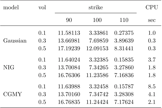
In Table 7 we report call option prices for weekly sampling, with risk-free rate 4% p.a., zero dividend yield and a year to maturity (S0 = 100; T = 1;

n = 50; r = 0:04, ^ = 0 and t = T =n in 5.1). Model parameters are given in Table 2. The precision of the reported numbers is 10 5. We can achieve higher precision (up to 10 8) by exploiting the regular quadratic convergence of our scheme in the number of gridpoints. Beyond10 8smooth convergence requires too many grid points to manage the computations in reasonable time.

Two comments are in order. Comparing leptokurtic prices with lognormal prices we …nd in-the-money options to be slightly more expensive while out-of-the-money options are substantially cheaper. This pattern is consistent with plain vanilla option prices (n= 1) and is caused by a combination of excess kurtosis and negative skew in the risk-neutral distribution. The same pattern is observed by Fusai and Meucci.

model vol strike CPU

90 100 110 sec

0.1 11.58113 3.33861 0.27375 1.0 Gaussian 0.3 13.66981 7.69859 3.89639 0.3 0.5 17.19239 12.09153 8.31441 0.3

0.1 11.64024 3.32385 0.15835 3.7 NIG 0.3 13.70084 7.34265 3.27860 1.8 0.5 16.76306 11.23586 7.16836 1.8

[image:16.612.170.443.116.299.2]

0.1 11.63988 3.32458 0.15787 8.5 CGMY 0.3 13.70160 7.34742 3.28308 4.1 0.5 16.76835 11.24424 7.17624 2.1

Table 7. Asian call option prices for Lévy log returns. Pre-cision 10 5. For detailed description of parameter values see main text. CPU timings in Matlab R15 on Dell Latitude 620 Intel Dual Core T7200, 2GHz, 2Gb RAM.

distribution (cf. equations 5.2, 5.3) are the primary factors driving option prices, while the choice of a speci…c parametric Lévy model plays a secondary role.

Appendix A. Fourier transform

De…nition A.1. Let f :_{R ! R} be an absolutely integrable function. The Fourier transform _F(f) :_R!Cis given by

F(f)(u) = Z ₁

1

f(s)eiusds: (A.1)

By slight abuse of notation we write _F(f(s)), even though the variables is immaterial. For example the Fourier transform of f(s) = g(s)e s would be denoted _F(g(s)e s_).

The inverse Fourier transform of g:_R!C is given by

F 1(g)(s) = lim

c!1

1 2

Z c

c

g(u)e iusdu

whenever the limit on the right hand side exists for all s_2R.

f =_F 1(_F(f)):

Proof. See Goldberg (1961), Theorem 5C.

Theorem A.3. If f1; f2 are absolutely integrable then

(f1 f2)(s) := Z ₁

1

f1(s0)f2(s s0)ds0 = Z ₁

1

f2(s0)f1(s s0)ds0

is absolutely integrable and

F(f1 f2) =F(f1)F(f2):

Proof. See Goldberg (1961), Theorems 7D, 7E.

Appendix B. Proofs

Proof of Theorem 3.1. 1) We will prove by induction onkthatE(X_n+_jGk) =

pk(ln(Xk n k))for k= 0; : : : ; n: The statement clearly holds fork =n:

Assume therefore that E(X_n+_jGk+1) =pk+1(ln(Xk+1 n k 1)) holds. By the law of iterated expectations

E(X_n+_jGk) =E(E(Xn+jGk+1)jGk) =E(pk+1(ln(Xk+1 n k 1))jGk):

Now substitute Xk+1 n k 1 =Xkexp(Zn k) from (2.3) to obtain

E(X_n+_jGk) = E(pk+1(lnXk+Zn k)jGk) =

Z

R

pk+1(lnXk+z)fk+1(z)dz = qk(lnXk) =pk(ln(Xk n k));

where the last two equalities follow from (3.2, 3.3). By induction therefore

E(X_n+) =E(X_n+_jG0) =q0(lnX0) =q0(ln n);

which completes the proof of the …rst assertion.

2) Since pn 0 and fk 0 for all k, it is obvious that pk; qk 0

for all k. We prove the upper bound by induction on k. The inequality

pk(y) akey +bk holds for k = n with an = 1 and bn = +₀: Assume

pk(y) akey+bk holds for arbitraryk 1:From (3.2)

qk 1(x) = Z

R

pk(x+z)fk(z)dz

Z

R

(akex+z+bk)fk(z)dz

= a_{k k}ex+bk=ak 1ex+bk;

which means (3.5) holds. Now use (3.3) to obtain

pk 1(y) = qk 1(ln(ey+ n k+1)) ak 1(ey+ n k+1) +bk

Proof of Theorem 3.2. 1) By induction onk we will prove

0 pk(x) p~k(x) ~akex+ ~bk forx2(Lk; Uk);0< k n, (B.1)

0 qk(x) q~k(x) a~k(ex n k) + ~bk forx2(Lk; Uk);0 k < n:

Inequality (B.1) holds trivially for k = n: Suppose it holds for arbitrary

k < n, then

qk 1(x) q~k 1(x) = Z

R

(pk(x+z) p~k(x+z))fk(z)dz 0:

Since (Lk 1; Uk 1) + (lk; uk) (Lk; Uk)we have

qk 1(x) q~k 1(x) = Z

[lk;uk]

(pk(x+z) p~k(x+z))fk(z)dz

+ Z

Rn[lk;uk]

(pk(x+z) p~k(x+z))fk(z)dz

Z

[lk;uk]

(~akex+z+ ~bk)fk(z)dz+

Z

Rn[lk;uk]

pk(x+z)fk(z)dz

Z

R

(~akex+z+ ~bk)fk(z)dz+

Z

Rn[lk;uk]

(akex+z+bk)fk(z)dz

= ~ak kex+ ~bk+akex(Fk(lk; 1) +Gk(uk; 1))

+bk(Fk(lk; 0) +Gk(uk; 0))

= ~ak 1ex+ ~bk 1 ~ak 1 n k+1

forx₂(Lk 1; Uk 1):Nowhk 1((Lk 1; Uk 1)) (Lk 1; Uk 1)which yields 0 pk 1(y) p~k 1(y) =qk 1(hk 1(y)) q~k 1(hk 1(y))

~

ak 1(ehk 1(y) n k+1) + ~bk 1= ~ak 1ey+ ~bk 1:

2, 3) The proof again proceeds by induction onk. Functionp~nis piecewise

di¤erentiable and satis…es (3.13). Assume (3.13) holds for arbitrary k < n:

Function0 p~0

k(x+z)fk(z)is dominated by an integrable function forxin a

compact interval therefore by Talvila (2001), Corollary 8 we can interchange integration and di¤erentiation to obtain

0 q~0_{k 1}(x) = Z

R

~

p0_k(x+z)fk(z)dz ak 1ex+ck forx2(Lk 1; Uk 1):

This in fact shows thatq~_k0 ₁(x)is continuous in(Lk 1; Uk 1):Sinceh0k 1(y)2 (0;1)for all y we also obtain

4) Fixk n: We have fk;p~k2L1(R) and let

g(x) = Z

R

~

pk(x+z)fk(z)dz = ~pk fk( z);

which by Young’s inequality is also in L1(_R). By the convolution theorem A.3,

F(g) =_F(~pk fk( z)) =F(~pk)F(fk( z)) =F(~pk) k:

By part 3) functions_fp~kgn_k=11;q~kare continuously di¤erentiable and bounded

on the interior of their support therefore we concludep~k;q~k are also of …nite

variation on every compact interval. Since g coincides with q~k 1 on the interior of its support by Fourier inversion theorem A.2 we obtain (3.2).

References

Andreasen, J. (1998). The pricing of discretely sampled Asian and look-back options: A change of numeraire approach. Journal of Computa-tional Finance 2(1), 5–30.

Bayraktar, E. and H. Xing (2008). Pricing Asian options for jump di¤u-sions. Available from http://arxiv.org/abs/0707.2432. To appear in Mathematical Finance.

Benhamou, E. (2002). Fast Fourier transform for discrete Asian options.

Journal of Computational Finance 6(1), 49–68.

Bluestein, L. I. (1968). A linear …ltering approach to the computation of the discrete Fourier transform. IEEE Northeast Electronics Research and Engineering Meeting 10, 218–219.

Carr, P., H. Geman, D. B. Madan, and M. Yor (2002). The …ne structure of asset returns: An empirical investigation. The Journal of Busi-ness 75(2), 305–332.

Carverhill, A. and L. Clewlow (1990). Flexible convolution. Risk 3(4), 25–29.

µ

Cerný, A. (2004). Introduction to FFT in …nance. Journal of Deriva-tives 12(1), 73–88.

Cont, R. and P. Tankov (2004).Financial Modelling with Jump Processes. Boca Raton: Chapman & Hall/CRC.

Fusai, G. and A. Meucci (2008). Pricing discretely monitored Asian op-tions under Lévy processes. Journal of Banking and Finance 32(10), 2076–2088.

Goldberg, R. R. (1961).Fourier transforms. Cambridge Tracts in Math-ematics and Mathematical Physics, No. 52. New York: Cambridge University Press.

Kemna, A. and T. Vorst (1990). A pricing method for options based on average asset values.Journal of Banking and Finance 14(1), 113–129. Kushner, H. J. and P. Dupuis (2001). Numerical Methods for Stochastic Control Problems in Continuous Time(2nd ed.). New York: Springer. Linetsky, V. (2004). Spectral expansions for Asian (average price) options.

Operations Research 52(6), 856–867.

Lord, R., F. Fang, F. Bervoets, and C. W. Oosterlee (2008). A fast and accurate FFT-based method for pricing early-exercise options under Lévy processes. SIAM Journal on Scienti…c Computing 30(4), 1678– 1705.

Madan, D., P. Carr, and E. Chang (1998). The variance gamma process and option pricing. European Finance Review 2(1), 79–105.

Rabiner, L. R., R. W. Schafer, and C. M. Rader (1969). The chirp z-transform algorithm and its application.Bell Systems Technical Jour-nal 48(5), 1249–1292.

Rogers, L. and Z. Shi (1995). The value of an Asian option. Journal of Applied Probability 32(4), 1077–1088.

Strawderman, R. L. (2004). Computing tail probabilities by numer-ical Fourier inversion: The absolutely continuous case. Statistica Sinica 14(1), 175–201.

Talvila, E. (2001). Necessary and su¢ cient conditions for di¤erentiating under the integral sign.The American Mathematical Monthly 108(6), 544–548.

Turnbull, S. and L. Wakeman (1991). A quick algorithm for pricing Eu-ropean average options. The Journal of Financial and Quantitative Analysis 26(2), 377–389.

Veµceµr, J. (2001). New pricing of Asian options.Journal of Computational Finance 4(4), 105–113.

Veµceµr, J. (2002). Uni…ed Asian pricing.Risk 15(6), 113–116.

Veµceµr, J. and M. Xu (2004). Pricing Asian options in a semimartingale model.Quantitative Finance 4(2), 170–175.

Cass Business School, City University London, 106 Bunhill Row, London EC1Y 8TZ, UK

E-mail address: [email protected]

URL:http://www.martingales.info

Cass Business School, City University London, 106 Bunhill Row, London EC1Y 8TZ, UK

E-mail address: [email protected]