Initial results on an MMSE precoding and equalisation approach to MIMO PLC channels

(1)

Initial Results on an MMSE Precoding and

Equalisation Approach to MIMO PLC Channels

Stephan Weiss

∗

, Nicola Moret

†

, Andrew P. Millar

∗

, Andrea Tonello

†

and Robert W. Stewart

∗

∗_{Dept of EEE, University of Strathclyde, Glasgow G1 1XW, Scotland, UK}

{stephan,bob}@eee.strath.ac.uk

†_{Dipartimento di Ingegneria Elettrica Gestionale Meccanica, Universit´a di Udine, Udine, Italy}

{nicola.moret, tonello}@uniud.it

Abstract—This paper addresses some initial experiments using polynomial matrix decompositions to construct MMSE precoders and equalisers for MIMO power line communications (PLC) channels. The proposed scheme is based on a Wiener formulation based on polynomial matrices, and recent results to design and implement such systems with polynomial matrix tools. Applied to the MIMO PLC channel, the strong spectral dynamics of the PLC system together with the long impulse responses contained in the MIMO system result in problems, such that diagonlisation and spectral majorisation is mostly achieved in bands of high energy, while low-energy bands can resist any diagonalisation efforts. We introduce the subband approach in order to deal with this problem. A representative example using a simulated MIMO PLC channel is presented.

I. INTRODUCTION

Many transceiver techniques such as OFDM or optimal filter bank based systems perform block processing [1], [2], whereby degrees of freedom are invested into a guard interval that enables to suppress inter-block interference (IBI). The remaining design can then utilise elegant linear algebraic techniques to achieve optimality in various senses, such as by employing a singular value decomposition of the resulting channel matrix. By applying IBI cancellation first rather than trading it off against various other system errors, error terms are not balanced. Recent systems considering this problem include e.g. [3], [4].

In this paper, we consider a minimum mean square error (MMSE) approach for filter bank design of precoding and equalisation targetting both inter-symbol interference (ISI) and structured noise that has been suggested in [5]. While [5] chooses an elegant polynomial matrix formulation, the lack of tools to address the resulting design problem have led to significant simplifications. Here, we explore the utilisation of a polynomial eigenvalue decomposition in [6], [7], which limits the precoder to a paraunitary design. The paraunitarity will be shown to have beneficial consequences, such as simple power control by well-known waterfilling algorithms [8], as well as the application of inversion techniques for polynomial matrices, which need to be solved for the precoder and equaliser design according to the Wiener approach in [5], [9]. The precoder and equalisation design is based on a formula-tion by Mertins [5], which is stated in Sec. III. In Sec. IV, some thoughts are provided on the implementation of this design. Inital results of this approach are discussed in Sec. V with an

application to simulated MIMO power line channel. Finally, conclusions are drawn in Sec. VI.

A. Notation

Below, boldface uppercase variables such asHwill indicate matrices, while boldface lowercase or underlined letters rep-resent vector valued variables, such as v orV. The operator {·}H_{indicates Hermitian transpose. For polynomial matrices,} such asH(z) =PnH[n]z

−n_{, the parahermitian operator}_{·}˜

implies Hermitian transpose of all matrices and time reversal, i.e. H˜(z) = HH(z−1_{) =} P

nHH[n]z n

. For abbreviation, transform pairs are denotedH(z)•—◦H[n]. The z-transform is here used for notational purposes only; no actual transfor-mation is carried out, and all calculations will be performed in the time domain.

II. SYSTEMMODEL

We assume a PLC channel utilising M wires for transmis-sion — e.g. phase, neutral, and earth in a single-phase system — with some degree of cross-coupling, such that anM×M

MIMO transmission system C[n]arises, whereby

C[n] =

     

c0,0[n] c0,1[n] . . . c0,M−1[n]

c1,0[n] c1,1[n] ...

..

. . .. ...

c(M−1),0[n] c(M−1),1[n] . . . c(M−1),(M−1)[n]

     

,

(1) with ci,j[n] being the channel impulse response between the

jth input and the ith output of the system. Additionally, we consider multiplexing P subchannels across the MIMO link C[n], which in term of notation can be represented by demultiplexing the channel C[n] into a M P ×M P matrix

H[n]. The structure of this channel matrix can be expressed in the z-domain based onC(z)•—◦C[n]by a block-pseudo-circulant polyphase descriptionH(z)•—◦H[n]

H(z) =

    

C0(z) z−1_CP

−1(z) . . . z

−1_C₁₍_z₎ ..

. . .. . .. ...

CP−2(z) C0(z) z −1_C

P−1(z)

CP−1(z) CP−2(z) . . . C0(z)

    

(2) whereCp(z) =P_nC[nP +p]z−n_.

(2)

ˆ

X

_[

n

_]

S

_[

n

_]

R

_[

n

_]

V

_[

n

_]

X

_[

n

_]

P

_[

n

_]

H

_[

n

_]

A

_[

n

_]

W

_[

n

_]

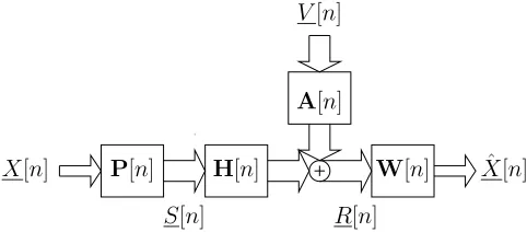
Fig. 1. System model with channel polyphase matrixH(z)and noise source

modelA(z); the transceiver design comprises of a precoder P(z) and an

equaliserW(z).

Besides co-channel interference (CCI) and ISI caused by

H(z), the received signal is affected by additive noise. Sim-ilar to the channel, the noise can be demultiplexed into P

subchannels. If the noise is Gaussian and broadband, then a source model or innovations filter matrix A(z) ∈ CM P×K

can linearly relate theM P noise signals corrupting the receive signal toKuncorrelated, mutually independent and identically distributed Gaussian processes with unit variance [10], which are denoted by V(z) ∈CK _•_—_◦v[m] in Fig. 1. Therefore, the noise power spectral matrix Rw(z)∈CK×K(z) as seen

at the receiver becomes

Rv(z) =A(z) ˜A(z) . (3)

As a consequence of (3),Rv(z)is parahermitian, i.e.Rv(z) = ˜

Rv(z).

The matrices P(z) ∈ CM P×N P₍_z₎ _and _W₍_z₎ _∈

CN P×M P₍_z₎_{describe the precoder and equaliser, respectively.}

Due to potential oversampling, i.e. N ≤ M, redundancy is introduced into the transmitted signal S[n], which can be exploited to mitigate structured noise and strong modes of the channel transfer function. The design of the linear precoder and equalisation systems P(z) and W(z) are the focus of this paper.

III. MMSE MIMO PRECODING ANDEQUALISATION

APPROACH

The precoder and equalisation design is based on a single-input single-output (SISO) formulation by Mertins [5]. For an arbitrarily selected precoder matrix P(z), according to a Wiener filter formulation in the z-domain in [5], the MMSE solution forW(z)can be stated as

W(z) =Re(z)·P˜(z) ˜H(z)R−1

v (z) , (4)

wherebyRe(z)is given by

Re(z) =σ2 h

I+σ2P˜(z) ˜H(z)R−1

v (z)H(z)P(z) i−1

, (5)

withσ2being the (equal) power of the signals inX[n]in Fig. 1 that feed into the precoder. Assuming that W(z) has been selected as in (4), the power spectral matrixRe(z)•—◦Re[τ]

defines the MMSE,ξMMSE, as

ξMMSE = tr{Re[0]} (6)

= tr

  

1 2π

2π Z

0

R(ejΩ)dΩ

  

. (7)

With W(z) selected as the Wiener solution according to (4), the precoder P(z)can be chosen such that the MSE in (6) is minimised. While in [5], the z-domain notation is chosen for its flexibility, the lack of polynomial matrix tools required a simplification for the solution by creating a non-polynomial precoder P0 = P(z). This is based on a trick exploited by most block-based transmission systems such as OFDM or optimal filter bank-based precoders and equalisers [1], [2], where the multiplexing factor P is selected larger than the channel order L.

With P > L, the polyphase components Cp(z) in (2)

become zero order, and the channel matrix H(z) reduces to a first order polynomial, where terms withz−1 _{are restricted} to the right upper triangular corner of H(z) as seen in (2). Using a guard interval, or employing leading or trailing zeros in the transmitter or receiver [1], [2] allows one to extract the zero order component of H(z). The insertion of a guard interval means that the filter bank is oversampled, and the degrees of freedom associated with the redundancy of this system are utilised to create a zero order transmission matrix thus eliminating IBI.

For the MMSE system in [5] defined by (4) and (5), an implicit selection of P > L leads to a rectangular — i.e. oversampled — selection P(z) = P0 such that the ex-pressionPH₀H˜(z)R−1

v (z)H(z)P0turns into a non-polynomial formulation.

IV. INVERSION OFPARAHERMITIANMATRICES

The work on an eigenvalue decomposition for polynomial matrices in [7] has stimulated a number of tools for polynomial matrix algebra such as the inversion of parahermitian matri-ces [11] required in (4) and (5), which can address the above MMSE formulation for precoder and equaliser more directy. The required tools are addressed below.

A. Polynomial Eigenvalue Decomposition

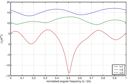
A polynomial eigenvalue decomposition of a parahermitian matrix R(z)∈CM×M₍_z₎_{is defined as}

R(z) =Q(z)Λ(z) ˜Q(z) (8)

wherebyQ(z)∈CM×M₍_z₎_{is paraunitary, i.e.}

Q(z) ˜Q(z) = ˜Q(z)Q(z) =I (9)

and Λ(z) ∈ CM×M₍_z₎ _{is parahermitian and diagonal with}

diagonal elementsΛi(z)ordered such that the power spectral

densities Λi(ejΩ)fulfill

Λi(ejΩ)≥Λi+1(ejΩ), ∀Ω, i= 0. . .(M−2) . (10)

[image:2.595.45.286.53.159.2]

(3)

0 0.1 0.2 0.3 0.4 0.5 0.6 0.7 0.8 0.9 1 −15

−10 −5 0 5 10 15 20

normalised angular frequency Ω / (2π)

|Λi

(e

j

Ω)|

[image:3.595.44.290.55.216.2]

i=1 i=2 i=3

Fig. 2. Power spectraΛi(ejΩ)of a spectrally majorised matrixR(z).

discussed later, an example a the spectrally majorisedΛ(z)is given in Fig. 2.

B. Polynomial Inverse

Based on the PEVD, the inverse can be formulated

R−1₍_z_{) =}_Q₍_z₎_Λ−1₍_z_{) ˜}_Q₍_z₎ _.

(11)

It is straightforward to show that

R−1₍_z₎_R₍_z_{) =}_R₍_z₎_R−1₍_z_{) =}_I _. ₍₁₂₎

The paraunitarity ofQ(z)plays a vital role in the simplicity of this inverse. It remains to invert the diagonal polynomial matrixΛ(z), which can be achieved by inverting all elements along on the main diagonal,

Λ−1₍_z_{) =}

    

Λ−1 0 (z)

Λ−1 1 (z)

. .. Λ−1

M−1(z)

    

, (13)

whereby Λi(z)Λ −1

i (z) = 1. Next, a practical decomposition

to determineQ(z)will be reviewed, before methods to invert the on-diagonal elementsΛi(z)are discussed in Sec. IV-D.

C. Sequential Best Rotation Algorithm

SBR2 is an iterative broadband eigenvalue decomposition technique based on second order statistics only and can be seen as a generalisation of the Jacobi algorithm. The decomposition afterL iterations is based on a paraunitary matrixUL(z),

UL(z) = L Y i=0

QiΓi(z) (14)

whereby Qi is a Jacobi rotation and the matrix Γi(z) a

paraunitary matrix of the form

Γi(z) =I−vivHi +z −∆i_v

ivHi (15)

with vi = [0 · · ·0 1 0 · · · 0]H _{containing zeros except for} a unit element in theδith position. Thus Γi(z)is an identity

matrix with the δith diagonal element replaced by a delay

z−∆i

.

At theith step, SBR2 will eliminate the largest off-diagonal element of the matrixUi−1(z)R(z) ˜Ui−1(z), which is defined by the two corresponding sub-channels and by a specific lag index. By delaying the two contributing sub-channels appropriately with respect to each other by selecting the position δi and the delay ∆i, the lag value is compensated.

Thereafter a Jacobi rotation Qi can eliminate the targetted

element such that the resulting two terms on the main diagonal are ordered in size, leading to a diagonalisation and at the same time accomplishing a spectral majorisation.

SBR2 only achieves an approximate diagonalisation after a finite number of iteration steps when off-diagonal elements are smaller than a threshold ϑ,

R(z) =Q(z) (Λ(z) +E(z)) ˜Q(z) (16)

with Λ(z) diagonal and E(z) a non-sparse error matrix with kE(z)k∞ ≤ ϑ. Here, the infinity norm kR(z)k∞ is defined as returning the largest element across all matrix-valued coefficients of the polynomialR(z),

kR(z)k∞= max

ν kRνk∞ . (17)

An alternative stopping criterion is to define a maximum number of iterations for SBR2 [6], [12].

D. Inversion of Autocorrelation Sequences

This section addresses the inversion of on-diagonal ele-ments of Λ(z). These elements have the properties of auto-correlation sequences, i.e.

rii[τ] =r

∗

ii[−τ]◦—•Rii(z) =R ∗ ii(z

−1₎ _.

This symmetry can be exploited in the inversion process, since the inverse of a linear phase SISO system must also be a linear phase system and therefore have the same symmetry properties [13]–[15]. From Rii(z)R

−1

ii (z) = 1 we deduce

rii[τ]∗sii[τ] =δ[τ]wheresii[τ]◦—•Sii(z) =R −1

ii (z)is the

inverse of the auto-correlation sequence. We here useS(z)to describe the inverse ofR(z)due to potential truncation errors in the methods described below.

E. Time Domain / MMSE Inversion

The time domain inversion is based on a convolutional matrix desciption of the convolution of an auto-correlation sequencer[n]and its inverses[n],

            

r[N]

.. . . ..

r[−N] r[N]

. .. . ..

r[−N] r[N]

. .. .._.

r[−N]

                    

s[−T]

.. .

s[0]

.. .

s[T]

       

=

           

0 .. . 0 1 0 .. . 0

           

(4)

or

As=d

with A ∈ C(2T+2N+1)×(2T+1)_, _s _∈ _C(2T+1) _and _d _∈

Z(2T+2N+1)_{. A solution can be obtained via the left} pseudo-inverse,

s= (AHA)−1

AHd (19)

This solution should have the same symmetry properties as r[n], and any deviation from symmetry must be due to numerical problems in the inversion process. The symmetry error

ǫ=ks−Js∗

k22 (20)

should be as small as possible.

A minimum mean square error solution to (19) can be ob-tained by including the noise-to-signal ratio for regularisation purposes.

1) Inversion with Explicit Symmetry Constraint: An ill-conditioned A can lead to an asymmetric solution in (19). Hence it is advantageous to enforce symmetry in the setup.

This can be performed by a Lagrangian approach, which solves the constrained optimisation problem

find min

s kAs−dk

2

2 (21)

subject to s=Js∗

. (22)

Instead of solving this Lagrangian problem, the next section discusses a direct approach of embedding the constraint into the formulation.

2) Inversion with Implicit Symmetry Constraint: The sym-metry condition can be incorporated into the system equation by formulating

Re{A} −Im{A} Im{A} Re{A}

·

Re{s} Im{s}

=

d

0

.

In this, the inverse is implicitly constrained by only defining half the response as

w=

    

s[−T]

.. .

s[1]

1 2s[0]

    

with

Re{s} =

 

IT 0 0T 2

JT 0 

Re{w}=M1Re{w} (23)

Im{s} =

 

IT 0 0T ₀

−JT 0 

Im{w}=M2Im{w} ,(24)

to reconstruct the real and imaginary part of the true solution. Therefore the problem formulation becomes

M1Re{A} −M2Im{A}

M2Im{A} M2Re{A}

| {z }

Ac

·

Re{w} Im{w}

=

d

0

| {z }

dc

0 200 400 600 800 1000

0 0.5 1 1.5 2 2.5

3x 10

−3

discrete time index n

|c00

[n]|

0 200 400 600 800 1000

0 0.5 1 1.5 2 2.5

3x 10

−3

|c01

[n]|

0 200 400 600 800 1000

0 0.5 1 1.5 2 2.5

3x 10

−3

|c10

[n]|

0 200 400 600 800 1000

0 0.5 1 1.5 2 2.5

3x 10

−3

|c11

[image:4.595.304.553.53.258.2]

[n]|

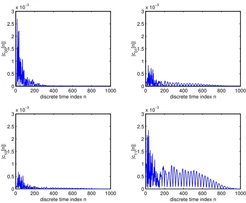
Fig. 3. PLC MIMO channel measurement sampleH₍ejΩ)over a frequency

range of 100MHz.

and the solution is reached via the pseudo-inverse

s= [M1 jM2] ATcAc −1

ATcdc .

The latter approach has been shown in [11] to be superior in terms of precision and computation complexity to both the unconstrained problem, as well as the formulation involving explicit constraints.

V. SIMULATIONS ANDRESULTS

In this section we present some initial results based on a MIMO PLC channel model developed at the University of Udine. This channel model generates channel responses based on a bottom-up PLC channel simulator described in [16]. A representative 2×2 MIMO channel characterised by the 4 magnitude responses of the constituting SISO subchannels

Cij(ejΩ)is shown in Fig. 3. The channel is simulated over a

bandwidth of 100MHz and exhibits severe frequency selectiv-ity.

Assuming a much simplified noise model with corruption by additive white Gaussian noise, the noise power spectral matrix is given by a scaled identity matrix, and the denominator of the Wiener solution yields

Re(z) = (I+σ2P˜(z) ˜H(z)H(z)P(z)) −1 _.

(25)

To minimise the MMSE, the terms in P˜(z) ˜H(z)H(z)P(z) need to be maximised, which can be achieved by constructing the precoder matrixP(z)to support the dominant polynomial eigenmodes ofH˜(z)H(z). We first attempt this directly using the H(z).

A. Direct Approach

[image:4.595.40.290.503.653.2]

(5)

−10000 −500 0 500 1000 0.5

1 1.5 2 2.5

x 10−4

lag τ

|r00

[

τ

]|

−10000 −500 0 500 1000

0.5 1 1.5 2 2.5

x 10−4

lag τ

|r01

[

τ

]|

−10000 −500 0 500 1000

0.5 1 1.5 2 2.5

x 10−4

lag τ

|r10

[

τ

]|

−10000 −500 0 500 1000

0.5 1 1.5 2 2.5

x 10−4

lag τ

|r11

[

τ

[image:5.595.40.552.52.259.2]

]|

Fig. 4. Space-time covariance matrixR_{= ˜}H₍z)H(z),

the MMSE is maximised, e.g. by selecting the strongest poly-nomial eigenmodes for transmission via P(z) by extracting the corresponding polynomial eigenvectors from Q(z) [17]. The advantage of this approach lies in the paraunitarity of the precoder matrix, thus preserving the transmit power, and the fact that the denominator remains an approximately diago-nalised matrix, therefore enabling a straightforward inversion according to Sec. IV-D.

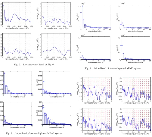
While the diagonalisation of the covariance matrix in Fig. 5 appears successful, inspecting the power spectral matrix

R(ejΩ₎_{in Fig. 6 reveals that the suppression of off-diagonal} terms is not great. Also, spectral majorisation is not satisfied across the entire frequency range. The reason can be found in Fig. 7, which shows the low-frequency component of the power spectral matrix, where a large term will dominate the MMSE calculations and therefore obstruct diagonalisation and spectral majorisation in frequency bands where the energy is low. In general, all of the simulated MIMO responses have revealed similar problems due to the very large dynamic range of the channel frequency responses.

The precoder would be designed from the paraunitary polynomial matrixU(z), such thatRe(z)is diagonal and can be inverted using the method described in Sec. IV-D, thus yielding the solution for the Wiener equaliser matrixW(z).

B. Subband Approach

In order to reduce the dynamic range, the MIMO system is combined with a filter bank based transmultiplexer similar to [18], whereby a decomposition into 14 bands oversampled by a factor 16 is achieved using an oversampled filter bank designed according to [11], [19]. The resulting MIMO systems in the 1st and 8th subband are shown in Figs. 8 and 9. Clearly the responses are significantly shorter, thus reducing the numerical complexity of the required polynomial matrix decompositions and inversions.

−10000 −500 0 500 1000

0.5 1 1.5 2 2.5

x 10−4

lag τ

|

γ00

[

τ

]|

−10000 −500 0 500 1000

0.5 1 1.5 2 2.5

x 10−4

lag τ

|

γ01

[

τ

]|

−10000 −500 0 500 1000

0.5 1 1.5 2 2.5

x 10−4

lag τ

|

γ10

[τ

]|

−10000 −500 0 500 1000

0.5 1 1.5 2 2.5

x 10−4

lag τ

|

γ11

[τ

[image:5.595.305.554.300.494.2]

]|

Fig. 5. Space-time covariance matrix in Fig. 4 after approximate

diagonali-sation by SBR2.

0 0.2 0.4 0.6 0.8 1

−140 −120 −100 −80 −60 −40 −20

20 log

10

|

Γ00

(e

j

Ω)|

normalised angular frequency Ω / π

0 0.2 0.4 0.6 0.8 1

−140 −120 −100 −80 −60 −40 −20

20 log

10

|

Γ01

(e

j

Ω)|

0 0.2 0.4 0.6 0.8 1

−140 −120 −100 −80 −60 −40 −20

20 log

10

|

Γ10

(e

j

Ω)|

0 0.2 0.4 0.6 0.8 1

−140 −120 −100 −80 −60 −40 −20

20 log

10

|

Γ11

(e

j

Ω)|

Fig. 6. Power spectral matrixΓ(z) = ˜U(z) ˜H(z)H(z)U(z)after

approx-imate diagonalisation by SBR2.

Fig. 10 depicts the 14 power spectral matrices arising from the transmultiplexer. This can be contrasted against the power spectra after applying SBR2 on the shortened MIMO system in each individual subband, resulting in the systems highlighted in Fig. 11. It is clear that compared to the fullband approach in Fig. 6, the subband approach can further reduce the off-diagonal components even at low gains in the presence of high-energy bands, yielding an improved diagonalisation by SBR2.

(6)

0 0.01 0.02 0.03 0.04 0.05 −90

−80 −70 −60 −50 −40 −30 −20

20 log

10

|

Γ00

(e

j

Ω)|

0 0.01 0.02 0.03 0.04 0.05 −90

−80 −70 −60 −50 −40 −30 −20

20 log

10

|

Γ01

(e

j

Ω)|

0 0.01 0.02 0.03 0.04 0.05 −90

−80 −70 −60 −50 −40 −30 −20

20 log

10

|

Γ10

(e

j

Ω)|

0 0.01 0.02 0.03 0.04 0.05 −90

−80 −70 −60 −50 −40 −30 −20

20 log

10

|

Γ11

(e

j

Ω)|

[image:6.595.51.556.48.503.2]

Fig. 7. Low frequency detail of Fig. 6.

0 10 20 30 40

0 0.002 0.004 0.006 0.008 0.01

|c0,00

[m]|

discrete time index m

0 10 20 30 40

0 0.002 0.004 0.006 0.008 0.01

|c0,01

[m]|

0 10 20 30 40

0 0.002 0.004 0.006 0.008 0.01

|c0,10

[m]|

0 10 20 30 40

0 0.002 0.004 0.006 0.008 0.01

|c0,11

[image:6.595.287.550.53.263.2]

[m]|

Fig. 8. 1st subband of transmultiplexed MIMO system.

polynomial matrix inversion according the concatenation of methods highlighted in this paper.

VI. CONCLUSION

Motivated by MMSE precoding and equalisation without block-processing, we have extended a Wiener filter formula-tion for polynomial matrices to the MIMO case and explored some polynomial matrix algrebra, in particular the inversion of polynomial matrices based on recent results derived from a polynomial eigenvalue decomposition used for the inversion of parahermitian matrices. The proposed approach has been tested on some simulated PLC MIMO channels.

The diagonalisation achieved in the representative example for a simulated MIMO PLC channel works well in regions with sufficiently high gain in the power spectral density. However, particularly at higher frequencies, which potentially can be gainfully employed for PLC, the diagonalisation is

0 5 10 15 20 25

0 0.5 1 1.5

x 10−3

|c7,00

[m]|

0 5 10 15 20 25

0 0.5 1 1.5

x 10−3

|c7,01

[m]|

0 5 10 15 20 25

0 0.5 1 1.5

x 10−3

|c7,10

[n]|

0 5 10 15 20 25

0 0.5 1 1.5

x 10−3

|c7,11

[m]|

Fig. 9. 8th subband of transmultiplexed MIMO system.

0 0.2 0.4 0.6 0.8 1

−140 −120 −100 −80 −60 −40 −20

20 log

10

|R

k,00

(e

j

Ω)|

normalised angular frequency Ω / (Kπ)

0 0.2 0.4 0.6 0.8 1

−140 −120 −100 −80 −60 −40 −20

20 log

10

|R

k,01

(e

j

Ω)|

0 0.2 0.4 0.6 0.8 1

−140 −120 −100 −80 −60 −40 −20

20 log

10

|R

k,10

(e

j

Ω)|

0 0.2 0.4 0.6 0.8 1

−140 −120 −100 −80 −60 −40 −20

20 log

10

|R

k,11

(e

j

Ω)|

Fig. 10. Concatenated power spectra across the 14 subbands of the

transmultiplexer.

[image:6.595.300.553.302.497.2]

(7)

0 0.2 0.4 0.6 0.8 1 −140

−120 −100 −80 −60 −40 −20

20 log

10

|

Γk,00

(e

j

Ω)|

0 0.2 0.4 0.6 0.8 1

−140 −120 −100 −80 −60 −40 −20

20 log

10

|

Γk,01

(e

j

Ω)|

0 0.2 0.4 0.6 0.8 1

−140 −120 −100 −80 −60 −40 −20

20 log

10

|

Γk,10

(e

j

Ω)|

0 0.2 0.4 0.6 0.8 1

−140 −120 −100 −80 −60 −40 −20

20 log

10

|

Γk,11

(e

j

Ω)|

[image:7.595.42.290.52.248.2]

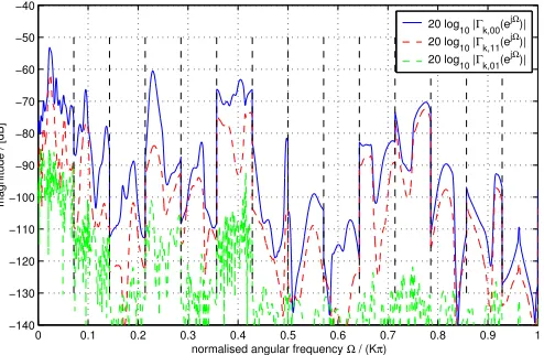
Fig. 11. Concatenated power spectra across the 14 subbands of the

transmultiplexed MIMO system diagonalised by SBR2 algorithms operating in every subband.

0 0.1 0.2 0.3 0.4 0.5 0.6 0.7 0.8 0.9 1

−140 −130 −120 −110 −100 −90 −80 −70 −60 −50 −40

magnitude / [dB]

20 log

10 |Γk,00(e jΩ_)|

20 log

10 |Γk,11(e jΩ_)|

20 log

10 |Γk,01(e jΩ_)|

Fig. 12. Overlaid power spectra of Fig. 11, highlighting the diagonalisaion

and spectral majorisation properties.

REFERENCES

[1] A. Scaglione, G. B. Giannakis, and S. Barbarossa, “Redundant Filter-bank Precoders and Equalizers. I. Unification and Optimal Designs,” IEEE Transactions on Signal Processing, vol. 47, no. 7, pp. 1988–2006, July 1999.

[2] ——, “Redundant Filterbank Precoders and Equalizers. II. Blind

Chan-nel Estimation, Synchronization, and Direct Equalization,”IEEE

Trans-actions on Signal Processing, vol. 47, no. 7, pp. 2007–2022, July 1999. [3] S. D’Alessandro, A. M. Tonello, and L. Lampe, “Bit-loading algorithms for OFDM with adaptive cyclic prefix length in PLC channels,” in IEEE International Symposium on Power Line Communications and Its Applications, Dresden, Mar./Apr. 2009, pp. 177–181.

[4] L. Vega and C. Galarza, “Redundancy reduced transceivers and channel

identification under impulsive noise,” inIEEE International Symposium

on Power Line Communications and Its Applications, March 2010, pp. 148–153.

[5] A. Mertins, “MMSE Design of Redundant FIR Precoders for Arbitrary

Channel Lengths,” IEEE Transactions on Signal Processing, vol. 51,

no. 9, pp. 2402–2409, September 2003.

[6] J. G. McWhirter and P. D. Baxter, “A Novel Technqiue for Broadband

SVD,” in12th Annual Workshop on Adaptive Sensor Array Processing,

MIT Lincoln Labs, Cambridge, MA, 2004.

[7] J. G. McWhirter, P. D. Baxter, T. Cooper, S. Redif, and J. Foster,

“An EVD Algorithm for Para-Hermitian Polynomial Matrices,” IEEE

Transactions on Signal Processing, vol. 55, no. 5, pp. 2158–2169, May 2007.

[8] D. P. Palomar and J. R. Fonollosa, “Practical Algorithms for a Family

of Waterfilling Solutions,” IEEE Transactions on Signal Processing,

vol. 53, no. 2, pp. 686–695, February 2005.

[9] C. Liu, S. Weiss, S. Redif, T. Cooper, L. Lampe, and J. G. McWhirter, “Channel Coding for Power Line Communication Based on

Oversam-pled Filter Banks,” in Proc. International Symposium on Power Line

Communications, L. Lampe, Ed., Vancouver, CA, April 2005, pp. 246– 249.

[10] A. Papoulis,Probability, Random Variables, and Stochastic Processes,

3rd ed. New York: McGraw-Hill, 1991.

[11] S. Weiss, A. Millar, and R. W. Stewart, “Inversion of parahermitian

ma-trices,” inEuropean Signal Processing Conference, Aalborg, Denmark,

August 2010, pp. 447–451.

[12] S. Redif and T. Cooper, “Paraunitary Filter Bank Design via a

Polyno-mial Singular Value Decomposition,” inProc. IEEE International

Con-ference on Acoustics, Speech, and Signal Processing, vol. 4, Philadel-phia, PA, March 2005, pp. 613–616.

[13] A. J. Kanto, “A formula for the inverse autocorrelation function of an

autoregressive process,” Journal of Time Series Analysis, vol. 8, pp.

311–312, 2008.

[14] W. S. Cleveland, “The inverse autocorrelations of a time series and

their applications,” Technometics, vol. 14, no. 2, pp. 277–293, May

1972. [Online]. Available: http://www.jstor.org/stable/1267420

[15] D. N. Politis, “Moving average processes and maximum entropy,”IEEE

Transactions on Information Theory, vol. 38, no. 3, pp. 1174–1177, May 1992.

[16] F. Versolatto, A.M. Tonello, “A MIMO PLC Random Channel Generator

and Capacity Analysis,” to appear inProc. International Symposium on

Power Line Communications, Udine, Italy, April 2011.

[17] S. Weiss, C. H. Ta, and C. Liu, “A Wiener Filter Approach to the Design of Filter Bank Based Single-Carrier Precoding and Equalisation,” in Proc. International Symposium on Power Line Communications, Pisa, Italy, Mar. 2007, pp. 493–498.

[18] N. Moret, A. Tonello, and S. Weiss, “Mimo precoding for filter bank modulation systems based on a polynomial singular value

decompo-sition,” in73rd Vehicular Technology Conference, Budapest, Hungary,

May 2011.

[image:7.595.44.291.301.462.2]