METHODS
GABRIEL R. BARRENECHEA AND FR´ED´ERIC VALENTIN
Abstract. This work establishes a formal derivation of local projection stabilized methods as a result of an enriched Petrov-Galerkin strategy for the Stokes problem. Both velocity and pressure finite element spaces are enhanced with solutions of residual-based local problems, and then the static condensation procedure is applied to derive new methods. The approach keeps degrees of freedom unchanged while gives rise to new stable and consistent methods for continuous and discontinuous approximation spaces for the pressure. The resulting methods do not need the use of a macro-element grid structure and are parameter-free. The numerical analysis is carried out showing optimal convergence in natural norms, and moreover, two ways of rendering the velocity field locally mass conservative are proposed. Some numerics validate the theoretical results.
1. Introduction
Residual of Euler-Lagrange equations have been involved in the the construction of finite element methods as a way to include the most desirable pair of spaces, namely the simplest and equal order elements, in the set of stable methods for the Stokes equation. Often adopted as an error indicator, residuals have the important property to vanish when finite solutions approach the exact ones. Thereby, when added to the standard Galerkin method, residual-dependent terms keep the approach consistent and the resulting methods, called stabilized methods, achieve optimal convergence rates.
Now, stabilized finite element methods for the Stokes problem have been criticized because of their need to set a constant, called the stabilization parameter. Some alternatives have been proposed to set up this constant among which is the enriching space approach. The idea is to enhance a pair of non stable finite element spaces and look for a discrete solution in the underlying augmented stable spaces through the standard Galerkin method. What drives the choice of additional basis functions is to fulfill the inf-sup condition without increasing the size of the corresponding linear system, i.e, without incorporating extra degrees of free-dom. A sufficient condition to respect the latter constraint is to perform static condensation
Key words and phrases. pressure polynomial projection methods, Stokes problem, local problem, consis-tent method.
procedure at the local level. This leads the enriched part of the numerical solution to be defined in terms of residuals and naturally incorporate them into the method. Moreover, this immediately establishes a bridge with stabilized methods where stabilized parameters are defined once and for all with respect to the integral of enriching basis functions. For instance, the equal order linear pair of spaces is made stable by adding bubble functions (re-sulting in the so-called mini-element, [3]) which might be related to a stabilized finite element method (see [21]). Ever since, literature on the subject has been steadily growing with the introduction of new techniques as the Residual-Free-Bubbles (RFB) [10, 9], the Variational Multiscale Methods (VMS) [19], and recently Petrov-Galerkin Enriched Methods (PGEM) [15, 4], just to name a few.
As an alternative to avoid this constant to set, in [13] a new type of methods, called polynomial pressure projection stabilized methods, have been developed (see also [7], where the analysis has been carried out). In fact, a parameter-free new stabilization term, based on the penalization of some projection error on the pressure, is added to the formulation in order to stabilize it. More precisely, if pl is the discrete polynomial pressure of order l, the method adds to the Galerkin method the following term (see next section for notations):
X
K∈Th
1
ν(pl−ρl−1(pl), ql−ρl−1(ql))K,
where ρl−1(ql) is the local L2 projection of ql onto space Pl−1(K) and ν ∈ R+. The stated
method can be seen as belonging to the class of Local Projection Stabilized (LPS) methods first introduced in [6]. Although similar, the method in [6] differs from the ones proposed in [13] since, rather than been based on fluctuations of the pressure, it involves the fluctuations of the gradient of pressure, and demands a parameter to be fixed. Some alternative forms of LPS methods have been proposed and analyzed inside a two-level approach (i.e., a dual coarser mesh is needed) [11], or based on an one-level strategy in [17] (see also [22] for a recent review and further references). What is common among all LPS methods is their lack of consistency, and the general strategy has been to prove that this remains bounded within the discretization error.
of local problems. Then, we apply the static condensation procedure to obtain new stabilized finite element methods which are now consistent (or weakly consistent for low order velocity approximations) and parameter free. In this work the extra term reads
X
K∈Th
1
ν(pl−ρ0(pl) +p
M
e (f −ν∆uk), ql−ρ0(ql))K,
plus appropriate jump terms if we use discontinuous pressure approximations, where uk stands for an order k polynomial velocity and pM
e (f −ν∆uk) belongs toL20(K) and solves
a local Stokes problem (see Section 2 for further details). At this point we just remark that the shape of the added terms prevents us from using the analysis from [11] since in our case the stabilization terms are no longer equivalent to P
K∈Thh2Kk∇plk20,K.
When applied to equal-order linear continuous interpolations for velocity and pressure we recover one of the methods given in [13] with a modified right hand side (in the case the pressure is approached using piecewise constant functions the method coincides with one of the methods proposed in [1]). Furthermore, this process gives a completely new method if the pressure is approximated using discontinuous linear functions. This method does not need a two-level strategy and also all the computations may be done at the element level, at the cost of enlarging the stencil of the matrix since now new jump terms appear in order to stabilize the discontinuities of the pressure. It is worth saying that jump terms (of a different nature) were already present in the LPS framework in [11] when discontinuous approximations of the pressure were used. We prove the method induces a positive definite linear system and leads to optimal convergence in natural norms.
Finally, the enrichment strategy suggests us two different ways to recover a locally mass conservative velocity field, an issue usually overlooked when solving the Stokes problem in the stabilized finite element context, but vital when it comes to couple the Stokes (or Navier-Stokes) equation with a heat or transport equation. We prove this fact and also prove that the addition of this new velocity field does not undermine the convergence of the method.
The plan of the paper is as follows: we end this section with some notations and definitions to be used throughout this manuscript. Next section is devoted to the presentation of the enriching space strategy and ends with the final form of the stabilized method. Section 3 exhibits the methods for three different choices of pairs of finite elements and includes a well-posedness result and error estimates for the new one. Numerical validations are in Section 4 and some conclusions are drawn in Section 5.
1.1. Preliminary notations. Let (·,·)D be the inner product in L2(D) (or in L2(D)2 or
L2(D)2×2, when necessary), and we denote by k· k
(or Hs(D)2, if necessary). As usual, H0(D) =L2(D), and |· |
0,D =k· k0,D. Also, H(div, D)
stands for the space of L2(D)2 functions whose divergence belongs to L2(D), provided with
the norm
kvkdiv,D :=
kvk20,D+k∇ ·vk20,D
1 2
.
Let Ω be an open bounded domain in R2 with polygonal boundary. A family of regular
triangulations of Ω reads {Th}h>0 , built up using triangles K with boundary ∂K,
charac-teristic length hK :=diam(K) and we denote h:= max{hK :K ∈ Th}. The set of internal edges F of the triangulation is denoted byEh with hF =|F|.
We denote n the normal outward vector on ∂K, ∂s and ∂n the tangential and normal
derivative operators, respectively, JvK stands for the jump of v across F, ΠS (denoted by ρ0
in the introduction), where S ⊂ R2, is the orthogonal projection onto the constant space, i.e.,
ΠS(q) := (q,1)S
|S| ,
(1)
and I is theR2×2 identity matrix.
In what followsVh stands for the usual finite element space of continuous piecewise linear polynomials with zero trace on∂Ω, andVh := [Vh]2. Also, Qlh denotes the space of piecewise polynomials of degree l, 0 ≤ l ≤ 1, which is continuous or discontinuous in Ω, and belong to L2
0(Ω). In addition, it will be useful in the sequel the orthogonal complement of Qlh in
L20(Th) denoted here by Gh, where we define the following broken spaces
H01(Th) := {v : v|K ∈H01(K)∀K ∈ Th},
L2
0(Th) := {v : v|K ∈L20(K)∀K ∈ Th}.
2. The model problem and the general framework
Let us consider the following Stokes problem:
−ν∆u + ∇p= f, ∇·u= 0 in Ω,
(2)
u= 0 on∂Ω,
where ν ∈R+ is the fluid viscosity and f ∈L2(Ω)2.
The continuous weak form of problem (2) over spaces [H1
0(Ω)2×L20(Ω)] satisfies the inf-sup
underlined pairs of spaces inf-sup stable through projection stabilized methods built up inside an enriching space strategy.
To this end, we start assuming that the design of interpolation basis functions must involve elemental residual of strong equations so as to incorporate missed features of exact solutions. This is not a strange approach as the whole class of stabilized and variational multiscale (inside which we include the RFB) methods are strongly based on this. What makes the present approach new is the way to involve residuals in the construction of basis functions which ultimately leads to a family of consistent stabilized projection methods.
Let us begin with a given initial unstable pair of interpolation spaces Vh×Ql
h as the trial and test spaces. By initial we mean that actual trial and test spaces are to be proposed enhancing Vh×Qlh. Since at this point no indication is available on how to set up enriched spaces, we augment initial space as ”big” as we can. As for the enriched trial spaces we perform it selecting
[Vh+H01(Ω)2]×[Qlh +L20(Th)],
thus the exact solution (u, p) is approached by
(uh, ph) := (u1+ue, pl+pe),
where (u1, pl) ∈ Vh ×Qlh and (ue, pe) ∈ H01(Ω)2 ×L20(Th). In regard to the enriched test
spaces, we set it up through the direct sum
[Vh⊕H01(Th)2]×[Qlh⊕Gh].
This choice makes a function (vh, qh) in it uniquely decomposed into (v1+vb, ql+qb), with (v1, ql)∈Vh×Qlh and (vb, qb)∈H01(Th)2×Gh.
Remark. Trial and test approximation spaces for pressure coincide forl = 0. Conformity of enriched velocity is assured imposing continuity of ue through a non homogenous transmis-sion condition on the internal edges (see equations (6)-(7)). In addition, the test space for the velocity is also conforming and test and trial spaces always differ to one another.
Next, we propose the following Petrov-Galerkin scheme for (2): Find (uh, ph) ∈ [Vh +
H1
0(Ω)2]×[Qlh+L20(Th)] such that
for allvh ∈Vh⊕H1
0(Th)2 and allqh ∈Qh⊕Gh. It follows straight from the Petrov-Galerkin scheme that it is equivalent to the following system:
ν(∇uh,∇v1)Ω−(ph,∇·v1)Ω+ (ql,∇·uh)Ω = (f,v1)Ω ∀(v1, ql)∈Vh×Qlh, (3)
ν(∇uh,∇vb)K−(ph,∇·vb)K + (qb,∇ ·uh)K = (f,vb)K, (4)
for all (vb, qb) ∈ H01(K)2 ×Gh, ∀K ∈ Th. Since ∇ ·u1|K ∈ R and vb|∂K = 0, and using a standard argument, equation (4) above corresponds to the weak form of the problem
−ν∆ue+∇pe =f +ν∆u1− ∇pl , ∇ ·ue ∈Pl(K) inK , (5)
where the residual of the first equation defines the right hand side. Now, to close this differential problem we start by fixing the boundary conditions on ue. To this end we impose the following boundary condition on ue:
(6) ue = ge on eachF ⊂∂K ,
where ge =0 if F ⊂∂Ω, and ge is the solution of
−ν ∂ssge =
α hF
ΠF(Jν∂nu1+plI·nK) inF ,
(7)
ge = 0 at the nodes,
on the internal edges, whereα ≥0. This boundary condition keeps the approach conforming and incorporates edge residuals close to those from the a posteriori error estimate given in [2].
Remark. The choiceα = 0 implies that the enrichment space for the velocity is composed of bubble functions which will turn out to be the correct way to stabilize continuous pressure spaces. For the case of discontinuous pressure spaces this constant will be set to α = 1.
Let us turn back to the local Stokes problems to compute (ue, pe). It emerges from (5) and (7) that (ue, pe) inherits the degrees of freedom of (u1, pl) and that it might be split into (ue, pe) = (uMe , pMe ) + (uGe, pGe) + (uDe , pDe) where each contribution satisfies, respectively,
−ν∆uMe +∇pMe =f +ν∆u1− ∇pl , ∇ ·uMe = 0 inK , (8)
uMe =0 on∂K ,
−ν∆uGe +∇pGe =0 , ∇ ·uGe ∈Pl(K) inK ,
(9)
and
−ν∆uDe +∇pDe =0 , ∇ ·uDe =
R
∂Kge·n
|K| inK ,
(10)
uDe =ge on∂K .
It remains to set problem (9). To this end, we first remark that, if f
K = (f1, f2) t ∈
R2, then the solution of (8) satisfies uMe =0 and pM
e =pMe (f +ν∆u1− ∇pl) is given by
pMe =f·x−ΠK(f·x) +pl−ΠK(pl)∈P1(K). (11)
Hence, we reinforce the dependence of enriching functions in terms of residual by closing (9) as follows:
−ν∆uGe +∇peG=0 , ∇ ·uGe =−1
ν p
M
e (f +ν∆u1− ∇pl) inK ,
(12)
uGe =0 on∂K .
It is worth remarking that (ue, pe) is uniquely defined through problems above and it satisfies equation (4). It remains then to fulfill equation (3). This, together with uMe = 0, lead to our method given by: Find (u1, pl)∈Vh×Ql
h such that
ν(∇u1,∇v1)Ω+ν X
K∈Th h
(∇uGe,∇v1)K + (∇uDe ,∇v1)K i
−(pl,∇ ·v1)Ω− X
K∈Th
(pe,∇ ·v1)K+ (ql,∇ ·u1)Ω
+ X
K∈Th h
(ql,∇ ·uGe)K+ (ql,∇ ·uDe )K
i
= (f,v1)Ω,
(13)
for all (v1, ql)∈Vh×Qlh.
Some of the terms in (13) can be simplified. First, integrating by parts and using that
uGe ∈H1
0(K)2 and ∆v1 = 0 in each K, we get
(∇uGe,∇v1)K = 0,
(∇uDe ,∇v1)K = (uDe , ν ∂nu1)∂K.
Furthermore, since pe ∈L20(K) we obtain
and from the characterization (11) we easily see that
(ql,∇ ·uGe)K = 1
ν(ql, pl−ΠK(pl))K−
1
ν(ql, p
M
e (f +ν∆u1))K
= 1
ν(ql−ΠK(ql), pl−ΠK(pl))K−
1
ν (ql−ΠK(ql), p
M
e (f +ν∆u1))K.
Finally, integrating by parts we further get
(ql,∇ ·uDe)K =−(∇ql,uDe)K+ (uDe, qlI·n)∂K.
Gathering last results, we rewrite (13) as: Find (u1, pl)∈Vh×Qlh such that
ν(∇u1,∇v1)Ω−(pl,∇ ·v1)Ω+ (ql,∇ ·u1)Ω
+1
ν
X
K∈Th
(pl−ΠK(pl) +pMe (−ν∆u1), ql−ΠK(ql))K−(∇ql,uDe )K
+ X
F∈Eh
(uDe ,Jν ∂nv1+qlI·nK)F = (f,v1)Ω+
1
ν
X
K∈Th
(pM
e (f), ql−ΠK(ql))K, (14)
for all (v1, ql)∈Vh×Qlh.
The edge contribution in method (14) rewrites in a more convenient form following [1]. In fact, since ΠF(Jν ∂nu1+plI·nK)
F is a constant function, thenge=α gFI·ΠF(Jν ∂nu1+plI·nK)
F, where gF stands for the solution of
(15) −ν ∂ssgF =
1
hF
inF , gF = 0 at the nodes,
on the internal edges.
Remark. It turns out that the solution of (15) may be calculated explicitly, in fact, is a polynomial of degree two in each one of the edges F. Then, since gF vanishes on the end-points ofF, and, forq∈P1(F) the function q−ΠF(q) vanishes on the mid-point ofF, using Simpson’s rule we obtain
(gF, q)F = (gF, q−ΠF(q))F + (gF,ΠF(q))F = (gF,ΠF(q))F .
Using this last remark we realize that the edge terms read
(uDe,Jν∂nv1+qlI·nK)F =
Z
F
gF
αΠF(Jν∂nu1+plI·nK)
F·ΠF(Jν∂nv1+qlI·nK)
F
= (gF,1)F
|F| α
ΠF(Jν∂nu1+plI·nK),ΠF(Jν∂nv1+qlI·nK)
F, with
(gF,1)F
|F| = hF 12ν.
Therefore, using this rewriting of the edge terms (14) becomes: Find (u1, pl) ∈ Vh ×Ql h
such that
ν(∇u1,∇v1)Ω−(pl,∇ ·v1)Ω+ (ql,∇ ·u1)Ω
+ X
K∈Th
(uDe,∇ql)K+ 1
ν
X
K∈Th
(pl−ΠK(pl) +pMe (−ν∆u1), ql−ΠK(ql))K
+ X
F∈Eh
αhF
12ν (ΠF(Jν ∂nu1+plI·nK),ΠF(Jν ∂nv1+qlI·nK))F
= (f,v1)Ω+
1
ν
X
K∈Th
(pMe (f), ql−ΠK(ql))K,
for all (v1, ql)∈Vh×Qlh.
Next, we highlight the new method above for different choices of interpolation spaces and characterize them with respect to known stabilized and local projection methods.
3. Applications
3.1. The simplest element P1×P0. In this case we consider α = 1 and then the method becomes: Find (u1, p0)∈Vh×Q0h such that
ν(∇u1,∇v1)Ω−(p0,∇ ·v1)Ω+ (q0,∇ ·u1)Ω
+ X
F∈Eh
hF
12ν(Jν∂nu1+p0I·nK,Jν∂nv1+q0I·nK)F = (f,v1)Ω,
(17)
for all (v1, q0)∈ Vh×Q0h, which is precisely one of the methods presented and analyzed in [1].
3.2. The element P1×P1 with continuous pressures. In this case we chooseα = 0 (i.e., we enrich the trial space with bubble functions), and use the fact that uDe =0to obtain the method: Find (u1, p1)∈Vh×Q1h such that
ν(∇u1,∇v1)Ω−(p1,∇ ·v1)Ω+ (q1,∇ ·u1)Ω
(18)
+1
ν
X
K∈Th
(p1−ΠK(p1) +pMe (−ν∆u1), q1−ΠK(q1))K = (f,v1)Ω+
1
ν
X
K∈Th
(pMe (f), q1−ΠK(q1))K,
3.3. The element P1 ×Pdisc
1 . The space of discrete pressures contains now discontinuous
functions. Then, considering α >0 the method reads: Find (u1, p1)∈Vh×Q1h such that
ν(∇u1,∇v1)Ω−(p1,∇ ·v1)Ω+ (q1,∇ ·u1)Ω
(19)
+1
ν
X
K∈Th
(p1−ΠK(p1) +pMe (−ν∆u1), q1−ΠK(q1))K+ X
K∈Th
(uDe ,∇q1)K
+ X
F∈Eh
α hF
12ν (ΠF(Jν ∂nu1+p1I·nK),ΠF(Jν ∂nv1+q1I·nK))F
= (f,v1)Ω+
1
ν
X
K∈Th
(pMe (f), q1−ΠK(q1))K,
(20)
for all (v1, q1) ∈ Vh ×Q1h. For reasons that will be detailed in the appendix, for α small enough we can neglect the term P
K∈Th(uDe ,∇q1)K and propose the following final form of
the method: Find (u1, p1)∈Vh×Q1h such that
B((u1, p1),(v1, q1)) = (f,v1)Ω+
1
ν
X
K∈Th
(pMe (f), q1−ΠK(q1))K,
(21)
for all (v1, q1)∈Vh×Q1h, where
B((u1, p1),(v1, q1)) :=ν(∇u1,∇v1)Ω−(p1,∇ ·v1)Ω+ (q1,∇ ·u1)Ω
(22)
+ 1
ν
X
K∈Th
(p1−ΠK(p1) +pMe (−ν∆u1), q1−ΠK(q1))K
+ X
F∈Eh
α hF
12ν (ΠF(Jν ∂nu1+p1I·nK),ΠF(Jν ∂nv1+q1I·nK))F .
Remark. The restriction on the value of α is done only to rigorously prove the link between the method and the enrichment strategy, so, from now on, we will consider α = 1 (which is the value used also in the numerical experiments). As a matter of fact, in the numerical experiments we have remarked virtually no impact of the value of α in the overall errors, and hence the choice α = 1 is completely justified.
Remark. The stated methods in this work may be classified as members of LPS family as long as we adopt low order pairs of spaces. As a matter of fact, when it comes to use them along with higher order polynomial interpolation such nomenclature is less clear as extra weak terms include the function pM
e (−ν∆uk) (responsible for making methods strongly consistent) instead of subtracting aL2 projection of pressure onto lower order finite element
3.4. Error analysis. The well-posedenees and consistency of the method are proved first. Let k · kh be the mesh-dependent norm given by
k(v1, q1)k2h :=ν|v1|21,Ω+
1
ν
X
K∈Th
kq1−ΠK(q1)k20,K +
X
F∈Eh
hF
12νkΠF(Jν∂nv1+q1I·nK)k
2 0,F. (23)
Then we present the following result.
Lemma 1. For all (v1, q1)∈Vh×Q1h there holds
B((v1, q1),(v1, q1)) =k(v1, q1)k2h, (24)
and (21) has a unique solution (u1, p1)∈Vh×Q1h. Let also (u, p)∈H2(Ω)2×H1(Ω) be the solution of (2) and (u1, p1) the solution of (21). Then
B((u−u1, p−p1),(v1, q1)) = 0,
(25)
for all (v1, q1)∈Vh×Q1h.
Proof. The first part is immediate from the definition of the bilinear form B(., .) in (22). For the consistency result we note that since u ∈ H2(Ω)2 and p ∈ H1(Ω) then J∂
nuK = 0
and JpK = 0, and the jump terms vanish. The consistency result follows recalling that
p−ΠK(p) =pM
e (∇p), and so the element wise enriching functionp−ΠK(p) +pMe (f−ν∆u)
in (21) also vanishes.
Before presenting the error estimate, we give the following technical result which will be useful in the sequel.
Lemma 2. Letv ∈L2(K)2 and let (uM
e (v), pMe (v)) be the solution of the problem
−ν∆uMe (v) +∇pMe (v) =v , ∇ ·uMe (v) = 0 inK ,
(26)
uMe (v) = 0 on∂K .
Then, there exists C >0, independent of h and ν, such that
ν|uMe (v)|1,K +kpeM(v)k0,K ≤C hKkvk0,K. (27)
Proof. First, from the weak formulation of (26) we see thatuMe (v) satisfies
ν|uMe (v)|2
Now, applying the Poincar´e inequality touM
e (v) we see thatkuMe (v)k0,K ≤ChK|uMe (v)|1,K, where C does not depend on h. Hence, we obtain
ν|uMe (v)|1,K ≤C hKkvk0,K. (28)
Next, from the inf-sup condition (cf. [16]), the weak form of problem (26) and applying once more the Poincar´e inequality in K and (28), we see that
kpMe (v)k0,K ≤β sup
w∈H01(K)2
−(pM
e ,∇ ·w)K
|w|1,K
=β sup
w∈H01(K)2
−ν(∇uM
e (v),∇w)K+ (v,w)K
|w|1,K
≤C βν|uMe (v)|1,K + hKkvk0,K
≤C β hKkvk0,K.
Finally, the inf-sup constant β >0 may be bounded as follows (cf. [16], Lemma III.3.1)
β ≤C
hK
R
2
1 + hK
R
,
(29)
where R is the diameter of any ball inscribed in K and C does not depend on K or hK.
Hence, the desired result arises using the mesh regularity of Th.
Now, we present the main error estimate. For this estimate, we introduce the Cl´ement interpolation operatorCh (cf. [12, 14]), with the obvious extension to vector-valued functions, satisfying
kv− Ch(v)kl,K ≤ C hKm−l|v|m,ωK,
(30)
kv− Ch(v)k0,F ≤ C h m−1
2
F |v|m,ωF ,
(31)
for all v ∈ Hm(Ω), where 0 ≤ l ≤ m, m = 1,2, and ω
K := ∪{K′ : K ∩ K′ 6= ∅},
ωF :=∪{K′ : F ∩K′ 6= ∅}. We recall some standard inequalities needed in the sequel (cf. [14]), namely, the local trace result: there exists C >0 such that
kvk20,F ≤C(h−1K kvk20,K +hK|v|21,K), (32)
for each edge F ⊂ ∂K and all v ∈ H1(K), and the inverse inequality: there exists C
I such that
CIhKk∇qk0,K ≤ kqk0,K, (33)
for all K ∈ Th and q ∈ P1(K). Finally, employing the latter and the generalized Poincar´e
inequality in each K (see [20]), it is easy to prove the following equivalence:
CIhK|q|1,K ≤ kq−ΠK(q)k0,K ≤
hK
π |q|1,K,
for all q ∈P1(K).
Theorem 3. Let us suppose that (u, p), solution of (2), belongs to H2(Ω)2 ×H1(Ω). Let
(u1, p1) be the solution of (21). Then, there exists C >0, independent of h and ν, such that
k(u−u1, p−p1)kh ≤C h
√
νkuk2,Ω+
1
√
ν |p|1,Ω
,
(35)
kp−p1k0,Ω ≤ Ch(νkuk2,Ω+|p|1,Ω).
(36)
Proof. Let ( ˜u1,p˜1) = (Ch(u),Ch(p)−ΠΩ(Ch(p))), (w1, q1) := (u1−u˜1, p1−p˜1) and (ηu, ηp) :=
(u−u˜1, p−p˜1). Then,
k(u−u1, p−p1)kh ≤ k(ηu, ηp)kh+k(w1, q1)kh. (37)
The first term may be bounded using (30)-(31) and the mesh regularity. In fact, we first remark that the interpolation error ηp also satisfies (30)-(31). Then, using that kq − ΠK(q)k0,K ≤ kqk0,K for all q ∈ L2(K), kΠF(q)k0,F ≤ kqk0,F, and the local trace result (32) we obtain
k(ηu
, ηp)k2h ≤ ν|ηu
|21,Ω+
1
ν
X
K∈Th
kηpk20,K + X F∈Eh
hF
12ν kJν∂nη u
+ηpI·nKk20,F
≤ ν|ηu
|21,Ω+
1
νkη
p
k20,Ω+C ν−1 X
K∈Th
kν∇ηu
+ηpIk20,K +h2K|ν∇u+ηpI|21,K
≤ C h2
ν|u|22,Ω+ 1
ν |p|
2 1,Ω
.
For the second term in (37) we use, respectively, Lemma 1, the Cauchy-Schwarz inequality and Lemma 2 to get
k(w1, q1)k2h = B((w1, q1),(w1, q1))
= B((ηu
, ηp),(w
1, q1))
= ν(∇ηu
,∇w1)Ω−(ηp,∇ ·w1)Ω+ (q1,∇ ·η
u )Ω +1 ν X K∈Th
(ηp−ΠK(ηp) +pMe (−ν∆u), q1−ΠK(q1))K
+ X
F∈Eh
hF
12ν(ΠF(Jν∂nη u
+ηpI·nK),ΠF(Jν∂nw1+q1I·nK))F
≤ ν|ηu
|1,Ω|w1|1,Ω+Ckηpk0,Ω|w1|1,Ω+ (q1,∇ ·ηu)Ω
+1
ν
X
K∈Th
kηp−ΠK(ηp)k0,K +kpMe (−ν∆u)k0,K
kq1−ΠK(q1)k0,K
+ X
F∈Eh
hF
12νkΠF(Jν∂nη u
+ηpI·nK)k0,FkΠF(Jν∂nw1+q1I·nK)k0,F
≤ C
(
k(ηu
, ηp)k2h+ 1
ν kη
p
k20,Ω+ X
K∈Th
νkpMe (∆u)k20,K
)12
k(w1, q1)kh+ (q1,∇ ·η
u
)Ω
≤ C
k(ηu
, ηp)k2
h+
h2
ν |p|
2
1,Ω+ν h2|u|22,Ω 12
k(w1, q1)kh+ (q1,∇ ·ηu)Ω
≤ C
k(ηu
, ηp)k2
h+
h2
ν |p|
2
1,Ω+ν h2|u|22,Ω
1 2
k(w1, q1)kh. (39)
The last step above deserves to be detailed. Integrating by parts and applying (30) we arrive at
(q1,∇ ·η
u
)Ω = − X
K∈Th
(∇q1, η
u
)K+
X
F∈Eh
(Jq1I·nK, ηu)F
≤ C X
K∈Th
h2K|q1|1,K|u|2,ωK + X
F∈Eh
kJq1I·nK−ΠF(Jq1I·nK)k0,Fkηuk0,F
+ X
F∈Eh
Next, we bound term by term. First, applying the equivalence result (34) and the mesh regularity we get
X
K∈Th
h2K|q1|1,K|u|2,ωK ≤ C (
X
K∈Th
kq1−ΠK(q1)k20,K
)12
h|u|2,Ω
≤ Ch√ν|u|2,Ωk(w1, q1)kh. (41)
For the second term we use the approximation properties of ΠF (cf. [14]), (31), the local trace result (32), the equivalence result (34) and the mesh regularity to obtain (as in (41))
X
F∈Eh
kJq1I·nK−ΠF(Jq1I·nK)k0,Fkηuk0,F ≤C
X
F∈Eh
h 5 2
F|Jq1K|1,F|u|2,ωF
≤ C
( X
K∈Th
h3K|q1|21,∂K
)12 (
X
F∈Eh
h2F |u|22,ωF )12
≤ C
( X
K∈Th
h2
K|q1|21,K
)
1 2
h|u|2,Ω
≤ Ch√ν|u|2,Ωk(w1, q1)kh. (42)
Finally, we treat the third term in (40) by similar arguments to get
X
F∈Eh
kΠF(Jq1I·nK)k0,Fkηuk0,F ≤
≤ C X
F∈Eh h 1 2 F
kΠF(Jν∂nw1+q1I·nK)k0,F +kΠF(Jν∂nw1K)k0,F
hF |u|2,ωF
≤C
( X
F∈Eh
hFkΠF(Jν∂nw1+q1I·nK)k
2 0,F +
X
K∈Th
hKkν∂nw1k
2 0,∂K
)12
h|u|2,Ω
≤C
(
k(w1, q1)k2h+
X
K∈Th
ν|w1|21,K
)12
h√ν|u|2,Ω.
(43)
Gathering contributions (41)-(43), equation (40) becomes
(q1,∇ ·η
u
)Ω ≤ C√ν h|u|2,Ωk(w1, q1)kh, (44)
which was the one used in (39). The first estimate result (35) follows using the interpolation error estimate (38) in (37).
Now we address (36). For that, we use that there exists (cf. [16]) w ∈H1
0(Ω)2 such that
then using consistency (25) applied to (w1,0) and integration by parts
kp−p1k20,Ω = (p−p1,∇ ·w)Ω
= X
K∈Th
(p−p1,∇ ·(w−w1))K+ (p−p1,∇ ·w1)Ω
= − X
K∈Th
(∇(p−p1),w−w1)K + X
F∈Eh
(J(p−p1)I·nK,w−w1)F
+ν(∇(u−u1),∇w1)Ω
+ X
F∈Eh
hF
12ν (ΠF(Jν∂n(u−u1) + (p−p1)I·nK),ΠF(Jν∂nw1K))F.
(45)
The next step is to bound each one of the terms above. To this end, we use (30) to proceed as in (41) to estimate the first term
X
K∈Th
(∇(p−p1),w−w1)K ≤C X
K∈Th
hK|p−p1|1,K|w|1,ωK
≤ C
( X
K∈Th
h2K|p|21,K +hK2 |p1−ΠK(p1)|21,K
)12
|w|1,Ω
≤ C
(
h2|p|21,Ω+ X K∈Th
kp1−ΠK(p1)k20,K
)12
|w|1,Ω
≤ C
(
h2|p|2 1,Ω+
X
K∈Th
kp−p1−ΠK(p−p1)k20,K +kp−ΠK(p)k20,K
)
1 2
|w|1,Ω
≤ C
h2
ν |p|
2
1,Ω+k(u−u1, p−p1)k2h
1
2 √
νkp−p1k0,Ω.
(46)
Using the Cauchy-Schwarz inequality combined with (31) and the mesh regularity we esti-mate the the second term by
X
F∈Eh
(J(p−p1)I·nK,w−w1)F
≤ X
F∈Eh
kJ(p−p1)I·nK−ΠF(J(p−p1)I·nK)k0,F +kΠF(J(p−p1)I·nK)k0,F
kw−w1k0,F
≤C
( X
F∈Eh
hF
kJp−p1K−ΠF(Jp−p1K)k20,F +kΠF(J(p−p1)I·nK)k20,F
)12
|w|1,Ω.
Now, to bound (47), recalling that the jump function on F = K ∩ K′ ∈ E
h satisfies ΠF(Jp−p1K) = ΠF((p−p1)|K)− ΠF((p−p1)|K′), and using the mesh regularity we
ob-tain (as in (46))
X
F∈Eh
hFkJp−p1K−ΠF(Jp−p1K)k20,F ≤C
X
K∈Th X
F⊆∂K∩Ω
hKkp−p1−ΠF(p−p1)k20,F
≤ C X
K∈Th X
F⊆∂K∩Ω
hKkp−p1 −ΠK(p−p1)k20,F
≤ C X
K∈Th
kp−p1−ΠK(p−p1)k02,K +h2K|p−p1|21,K
≤ C ν
k(u−u1, p−p1)k2h+
h2
ν |p|
2 1,Ω
.
(48)
Similarly, we prove that
X
F∈Eh
hFkΠF(J(p−p1)I·nK)k20,F
≤ X
F∈Eh
hFkΠF(Jν∂n(u−u1) + (p−p1)I·nK)k
2
0,F +kΠF(Jν∂n(u−u1)K)k
2 0,F
≤ C ν(k(u−u1, p−p1)k2h+ν h2|u|22,Ω).
(49)
Hence, (47) becomes
X
F∈Eh
(J(p−p1)I·nK,w−w1)F
≤ C√ν
k(u−u1, p−p1)k2h+ν h2|u|22,Ω+
h2
ν |p|
2 1,Ω
12
kp−p1k0,Ω.
(50)
The last term in (45) is tackled using Cauchy-Schwarz’s inequality leading to
ν(∇(u−u1),∇w1)Ω+ X
F∈Eh
hF
12ν (ΠF(Jν∂n(u−u1) + (p−p1)I·nK),ΠF(Jν∂nw1K))F
≤Ck(u−u1, p−p1)kh√νkp−p1k0,Ω.
(51)
Finally, gathering contributions (46), (50) and (51) we end up with
kp−p1k20,Ω ≤C
√ ν
k(u−u1, p−p1)k2h+
h2
ν |p|
2
1,Ω+ν h2|u|2,Ω
1 2
kp−p1k0,Ω,
(52)
and the result follows dividing by kp−p1k0,Ω and using (35).
Lemma 4. Let us suppose that Ω is a convex polygon. Then, there existsC >0, independent of h and ν, such that
ku−u1k0,Ω ≤C h2
|u|2,Ω+
1
ν|p|1,Ω
.
(53)
Proof. We consider the dual problem
−ν∆ψ− ∇ξ=u−u1 , ∇ ·ψ = 0 in Ω,
(54)
ψ=0 on∂Ω.
Since Ω is a convex polygon, then (ψ, ξ)∈H2(Ω)2×H1(Ω), and the following estimate holds
νkψk2,Ω+kξk1,Ω ≤ Cku−u1k0,Ω.
(55)
Now, multiplying the first equation in (54) byu−u1, the second one by−(p−p1), integrating
by parts, using the definition ofB(., .) and the fact that J∂nψK=0 and JξK = 0 we obtain
ku−u1k20,Ω = ν(∇(u−u1),∇ψ)Ω−(p−p1,∇ ·ψ)Ω+ (ξ,∇ ·(u−u1))Ω
= B((u−u1, p−p1),(ψ, ξ))−
1
ν
X
K∈Th
(p−p1−ΠK(p−p1) +pMe (−ν∆u), ξ−ΠK(ξ))K.
Now, we define ψ1 :=Ch(ψ) and ξ1 :=Ch(ξ)−ΠΩ(Ch(ξ)). Then, using the Cauchy-Schwarz inequality, (32) and (30), we arrive at
ku−u1k20,Ω = B((u−u1, p−p1),(ψ−ψ1, ξ−ξ1))
− 1 ν
X
K∈Th
(p−p1−ΠK(p−p1) +pMe (−ν∆u), ξ−ΠK(ξ))K
≤ C
(
k(u−u1, p−p1)k2h+ 1
νkp−p1k
2 0,Ω+
1
ν
X
K∈Th
ν2kpM
e (∆u)k20,K
)
1 2
(
k(ψ−ψ1, ξ−ξ1)k2h+ 1
ν kξ−ξ1k
2 0,Ω+
1
ν
X
K∈Th
kξ−ΠK(ξ)k20,K
)12 ,
and the result follows using (38),(30), the approximation properties of ΠK(cf. [14]), (55),(35),
(36), Lemma 2 and dividing by ku−u1k0,Ω.
point that the results presented in this section may be directly applied to the P1/P0 method from §3.1). First, as in [4] we can consider uDe given as the solution of (10) (with α = 1) and get an enriched velocity field ˜uh :=u1+uDe , satisfying the following result.
Lemma 5. Let ˜uh := u1 + uDe, where u1 and uDe are the solutions of (21) and (10), respectively. Then,
∇ ·u˜h = 0 ∀K ∈ Th. (56)
Moreover, if (u, p) ∈ H2(Ω)2 ×H1(Ω) is the solution of (2), then there exists a constant
C >0, independent of h and ν, such that
|u−u˜h|1,Ω ≤ Ch
kuk2,Ω+
1
ν|p|1,Ω
,
(57)
and, assuming Ω a convex polygon, the following estimate holds
ku−u˜hk0,Ω ≤ Ch2
kuk2,Ω+
1
ν |p|1,Ω
.
(58)
Proof. LetK′ ∈ T
h be a fixed element andK any other element of the triangulation, and let us define the functionq1 ∈Q1h as follows: q1 = 1 inK′,q1 =−|K
′|
|K| inK, and zero everywhere
else. Then, using (0, q1) as test function in the definition of the method (cf. (21)) we get
(q1,∇ ·u1)K∪K′ +
X
F∈Eh
hF
12ν(ΠF(Jν∂nu1+p1I·nK),Jq1I·nK)F = 0,
(59)
and then, integrating by parts and using (10) we obtain
(1,∇ ·(u1 +uDe ))K =
|K|
|K′|(1,∇ ·(u1+u
D e))K′.
(60)
Now, since (u1+uDe)·n= 0 on ∂Ω we have
0 = (1,∇ ·(u1+uDe ))Ω = (
X
K∈Th
|K| |K′|
)
(1,∇ ·(u1+uDe ))K′,
(61)
leading to (1,∇ ·(u1+uDe ))K′ = 0. The result follows using that∇ ·(u1+uDe )∈R in each
element of Th.
The proof of the error estimate reduces to prove a bound for |uDe |1,K in each K ∈ Th. To do this, we multiply (10) by uDe , integrate by parts, use that kv ·nk−1
[18]), and (10) to obtain that
ν|uDe |21,K = −(uDe ,−ν ∂nu
D
e +pDeI·n)∂K
≤ kuDek1
2,∂Kk −ν∂nu
D
e +pDeI·nk−1 2,∂K ≤ kgek1
2,∂K
k −ν∇uDe +pDe Ik20,K+k∇ ·(−ν∇uDe +pDeI)k20,K
1 2
≤ Ckgek1
2,∂K ν|u
D
e |1,K +kpDe k0,K
.
(62)
Next, following analogous steps as in the proof of Lemma 2, we obtain that there exists a constant C >0, independent of hK, such that
kpDek0,K ≤C ν|uDe |1,K, (63)
and then, there exists C > 0, independent of h, such that
|uDe |1,K ≤Ckgek1 2,∂K,
and sincege is a polynomial of degree two in each edge, we use an inverse estimate (cf. [14]) to see that kgek1
2,∂K ≤C h
−1 2
K kgek0,∂K, leading to
|uDe|1,K ≤C h− 1 2
K kgek0,∂K. (64)
In addition, since ge|F =gF I·ΠF(Jν∂nu1+p1I·nK|F), where gF satisfies gF ≤C ν
−1h
F in F, then
kgek20,F ≤ Z
F
gF2 |ΠF(Jν ∂nu1+p1I·nK)|
2
≤ C h
2
F
ν2 kΠF(Jν∂nu1+p1I·nK)k
2 0,F. (65)
Hence, using (65), (64) leads to
|uDe |1,K ≤ C h− 1 2
K
( X
F⊂∂K∩Ω
h2
F
ν2 kΠF(Jν ∂nu1+p1I·nK)k
2 0,F
)
1 2
≤ √C ν
( X
F⊂∂K∩Ω
hF
ν kΠF(Jν ∂nu1+p1I·nK)k
2 0,F
)12 .
Then, squaring, summing over all the triangles ofTh, using that J∂nuK =0 and JpK= 0 and
(35) we obtain
|uDe|1,K ≤ C ν−12
( X
F∈Eh
hF
12νkΠF(Jν ∂n(u−u1) + (p−p1)I·nK)k
2 0,F
)
1 2
≤ C ν−12 k(u−u
1, p−p1)kh
≤ Ch
|u|2,Ω+
1
ν|p|1,Ω
,
(67)
and (57) follows. To prove (58) we first remark that, for a function v ∈H1(K), a standard
scaling argument leads to the following generalized Poincar´e inequality
kvk0,K ≤ C hK |v|1,K +
X
F⊂∂K
h− 1 2
F kvk0,F
!
,
(68)
where C >0 does not depend on hK. Applying this result to uDe and using (65) we obtain
kuDek0,K ≤ C hK |uDe |1,K +
X
F⊂∂K∩Ω
h− 1 2
F kgek0,F
!
≤ C hK |uDe |1,K +
X
F⊂∂K∩Ω
h 1 2
F
ν kΠF(Jν∂nu1+p1I·nK)k0,F
!
,
(69)
and then (58) follows using the same arguments as for (67).
This first approach has the advantage of providing a continuous velocity field, with the same nodal values as u1, but at the cost of solving the local problem (10) as a post-process
after the solution. To avoid this local problem solutions, we define in each K ∈ Th (see [5] for a related idea)
unc =
X
F⊂∂K∩Ω
hF
12νΠF(Jν∂nu1+p1I·nK
F)ϕF, (70)
where ϕF is the basis function of the lowest order Raviart-Thomas space given by
ϕF(x) = hF
2|K|(x−xF),
(71)
Lemma 6. Let u1 be the solution of (21) andunc given in (70), respectively. The velocity field ¯uh :=u1+unc satisfies
∇ ·u¯h = 0 in each K ∈ Th.
Furthermore, being (u, p)∈H2(Ω)2×H1(Ω) the solution of (2), the following error estimate
is valid
( X
K∈Th
|u−u¯h|21,K
)12
≤ Ch
kuk2,Ω+
1
ν|p|1,Ω
,
(72)
whereC >0 neither depend onhnorν. In the case that Ω is a convex polygon, the following estimate holds
ku−u¯hk0,Ω ≤Ch2
kuk2,Ω+
1
ν |p|1,Ω
.
(73)
Proof. The local conservation of mass arises as in the previous Lemma. For the error estimate we first remark that, due to the mesh regularity and the definition ofϕF (cf. (71)),|ϕF|1,K ≤
C, and then using the Cauchy-Schwarz inequality and J∂nuK=0, JpK= 0, we arrive at
|unc|1,K ≤C X
F⊂∂K
hF
ν
ΠF(Jν∂nu1+p1I·nK)|F
= C
ν
X
F⊂∂K
Z
F|
ΠF(Jν∂nu1+p1I·nK)|
≤ Cν X
F⊂∂K
h 1 2
F kΠF(Jν∂nu1+p1I·nK)k0,F
≤ C ν
X
F⊂∂K
h 1 2
FkΠF(Jν∂n(u−u1) + (p−p1)I·nK)k0,F,
(74)
and (72) follows as in (67). Finally, the estimate forku−u¯hk0,Ω is done following the exact
same steps and using that kϕFk0,K ≤ChK.
4. A numerical experiment
Before heading to the numerical experiments, we make a short remark on the final imple-mentation of the method. If the functionf is not a piecewise constant, then we must be able to solve problem (8) before implementing the method, thus, leading to a two-level method. If we want to avoid this, we can approximate f by ΠK(f) in each element and just use the analytical solution from (11). Now, this approximation introduces a consistency error, but, we can prove that it is of a smaller order. In fact, let us suppose that f ∈ H1(Ω)2 and let
Then, using the Lemma 2, Cauchy-Schwarz’s inequality and the approximation properties of ΠK (cf. [14]), we obtain
k(u1 −u˜1, p1−p˜1)k2h = B((u1−u˜1, p1−p˜1),(u1−u˜1, p1−p˜1))
= 1
ν
X
K∈Th
(pMe (f)−pMe (ΠK(f)), p1−p˜1−ΠK(p1−p˜1))K
≤ 1 ν
X
K∈Th
kpM
e (f)−pMe (ΠK(f))k0,Kkp1−p˜1−ΠK(p1−p˜1)k0,K
≤ √1 ν
( X
K∈Th
kpMe (f −ΠK(f))k20,K
)12
k(u1−u˜1, p1−p˜1)kh
≤ √1 ν
( X
K∈Th
C h2Kkf −ΠK(f)k2 0,K
)12
k(u1 −u˜1, p1−p˜1)kh
≤ √1 ν
( X
K∈Th
C h4K|f|21,K )12
k(u1−u˜1, p1−p˜1)kh,
and then, dividing by k(u1−u˜1, p1−p˜1)kh we arrive at
k(u1−u˜1, p1−p˜1)kh ≤C
h2
√
ν |f|1,Ω,
(75)
and both solutions are superclose and the loss of convergence (and consistency) due to the approximation of f by ΠK(f) is of one order smaller than the order of the method.
Now, we test the performance of our methods with the analytical solution
u(x, y) = −256x
2(x−1)2y(y−1)(2y−1)
256y2(y−1)2x(x−1)(2x−1) !
,
(76)
p(x, y) = 150(x−0.5)(y−0.5).
(77)
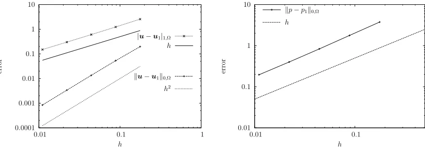
In Figure 1 we depict the convergence history for the method using continuous pressure interpolations and in Figure 2 the convergence history for the method with discontinuous interpolations. We observe that both errors go to zero as predicted by the theory, and the continuous pressure interpolation case achieves even better results. This fact has already been observed in [13] and deserves further investigations.
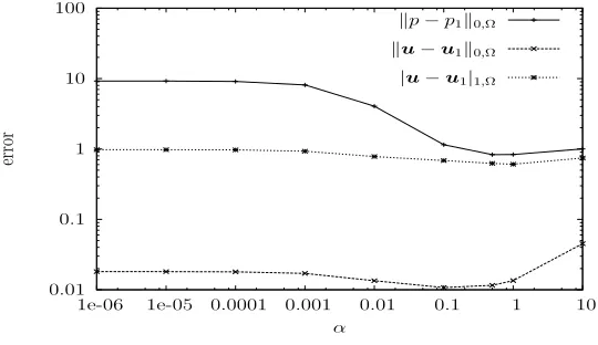
Finally, in Figure 3 we depict the errors of the method (21) with respect to the parameter
errors. In fact, whenα varies from 10−6 to 10 we see that the errors vary at most of an order
of 10, and hence our choice of α= 1 is completely justified.
0.0001 0.001 0.01 0.1 1 10
0.01 0.1 1
er
ro
r
h
h
ku−u1k0,Ω
h2
|u−u1|1,Ω
0.01 0.1 1 10
0.01 0.1 1
er
ro
r
h
kp−p1k0,Ω
h3
[image:24.612.84.530.196.355.2]2
Figure 1. Convergence history of the method (18) (continuous pressures).
0.0001 0.001 0.01 0.1 1 10
0.01 0.1 1
er
ro
r
h
h
ku−u1k0,Ω
h2
|u−u1|1,Ω
0.01 0.1 1 10
0.01 0.1
er
ro
r
h kp−p1k0,Ω
h
[image:24.612.85.523.532.689.2]0.01 0.1 1 10 100
1e-06 1e-05 0.0001 0.001 0.01 0.1 1 10
er
ro
r
α
kp−p1k0,Ω
ku−u1k0,Ω
[image:25.612.170.440.99.255.2]|u−u1|1,Ω
Figure 3. Errors of the method (21) with respect to α.
5. Conclusion
The focus of this work was to establish local projection methods inside an enriching frame-work relied on residuals. The new way to incorporate them inside a Petrov-Galerkin approach was the key ingredient to achieve stable and consistent new version of LPS (or polynomial projection methods) and still maintain them parameter-free, and without the need of a dual coarser mesh satisfying a macro-element property. We also took advantage of the enhanced space approach to propose a way to recover a locally mass conservative velocity field with and without additional computational cost. Our analysis and numerical validations were limited to piecewise linear continuos and discontinuous interpolation spaces, although the approach is not restricted to them. In the latter case, completely new methods arise for which the denomination of LPS methods is no longer adequate, and for which the Laplacian term no longer vanishes, thus making them strongly consistent. This, as well as extension of the present framework to other problems, such as the Navier-Stokes equation, will be the subject of future research.
6. Appendix
Having disregard the term P
K∈Th(uDe ,∇q1)K in the original method (19) we show here
that the procedure does not impact error optimality. This is addressed in the following result:
Theorem 7. Let us suppose that (u, p), solution of (2), belongs to H2(Ω)2 ×H1(Ω).
exists C, C1 >0, independent of h and ν, such that for α < C1 there holds
k( ˆu1−u1,pˆ1−p1)kh ≤C h
√
νkuk2,Ω+√1
ν |p|1,Ω
.
(78)
Proof. We note the original bilinear form by ˆB(., .), i.e.,
ˆ
B((u1, p1),(v1, q1)) := B((u1, p1),(v1, q1)) + X
K∈Th
(uDe,∇q1)K,
where B(., .) is defined in (22). Stability and consistency for the method (19) must be established before heading to prove the error result. For that, we first remark that replacing (66) in (69) and using mesh regularity the following estimate holds for uDe =uDe((v1, q1)):
kuDe k0,K ≤C hK
X
F⊆∂K∩Ω
α h 1 2
F
ν kΠF(Jν ∂nv1+q1I·nK)k0,F for all K ∈ Th.
Hence, from the definition of ˆB(., .), the Cauchy-Schwarz inequality, (34) and the above estimate we get
ˆ
B((v1, q1),(v1, q1)) =k(v1, q1)k2h+
X
K∈Th
(uDe ,∇q1)K
≥ k(v1, q1)k2h−
X
K∈Th
kuDek0,Kk∇q1k0,K
≥ k(v1, q1)k2h−
X
K∈Th
kuDek0,KCI−1hK−1kq1−ΠK(q1)k0,K
≥ k(v1, q1)k2h−C
X
K∈Th X
F⊆∂K∩Ω
α h1F/2
ν kΠF(Jν ∂nv1+q1I·nK)k0,FC
−1
I kq1−ΠK(q1)k0,K
≥ k(v1, q1)k2h−
C2
2γk(v1, q1)k
2
h−
α γ
2C2
I
k(v1, q1)k2h
=
1− C
2
2γ − αγ
2C2
I
k(v1, q1)k2h,
and the coercivity result follows setting γ = C2 and α < (CI
C)
2. In addition, since method
We are ready to prove the error estimate. Using previous results and the estimate for
uDe =uDe((u−u1, p−p1)) given in (69) we get
Ck( ˆu1−u1,pˆ1−p1)k2h ≤Bˆ(( ˆu1−u1,pˆ1−p1),( ˆu1 −u1,pˆ1−p1))
= ˆB((u−u1, p−p1),( ˆu1−u1,pˆ1−p1))
= X
K∈Th
(uDe,∇(ˆp1−p1))K
≤ X
K∈Th
kuDek0,KCI−1h−1K kpˆ1−ΠK(ˆp1)−p1+ ΠK(p1)k0,K
≤C h
ν|u|2,Ω+ 1
ν|p|1,Ω
k( ˆu1−u1,pˆ1−p1)kh,
and the result follows by dividing both sides byk( ˆu1−u1,pˆ1−p1)khand reordering constants.
Remark. Convergence rates of order h and h2 for the errors kpˆ
1 −p1k0,Ω and kuˆ1 −u1k0,Ω
may be accomplish following proof of Theorem 3 and Lemma 4, respectively.
References
[1] R. Araya, G. R. Barrenechea, and F. Valentin, Stabilized finite element methods based on multiscale enrichment for the Stokes problem, SIAM J. Numer. Anal., 44 (2006), pp. 322–348.
[2] , A stabilized finite element method for the Stokes problem including element and edge residuals, IMA Journal of Numerical Analysis, 27 (2007), pp. 172–197.
[3] D. Arnold, F. Brezzi, and M. Fortin,A stable finite element for the Stokes equations, Calcolo, 21 (1984), pp. 337–344.
[4] G. R. Barrenechea, L. P. Franca, and F. Valentin,A Petrov-Galerkin enriched method: a mass conservative finite element method for the Darcy equation, Computer Methods in Applied Mechanics and Engineering, 196 (2007), pp. 2449–2464.
[5] ,A symmetric nodal conservative finite element method for the Darcy equation. Preprint 2008-07, Department of Mathematics, University of Strathclyde, 2008.
[6] R. Becker and M. Braack,A finite element pressure gradient stabilization for the Stokes equations based on local projections, Calcolo, (2001), pp. 173–199.
[7] P. Bochev, C. Dohrmann, and M. Gunzburger,Stabilization of low-order finite elements for the Stokes problem, SIAM J. Numer. Anal., 44 (2006), pp. 82–101.
[8] M. Braack and E. Burman,Local projection stabilization for the Oseen problem and its interpretation as Variational Multiscale Method, SIAM J. Numer. Anal., 43 (2006), pp. 2544–2566.
[9] F. Brezzi, L. Franca, T. J. Hughes, and A. Russo, b = R
g, Comput. Methods Appl. Mech. Engrg., 145 (1997), pp. 329–339.
[11] E. Burman, Pressure projection stabilizations for Galerkin approximations of Stokes’ and Darcy’s problem, Numer. Methods Partial Differential Eq., 24 (2008), pp. 127–143.
[12] P. Cl´ement, Approximation by finite element functions using local regularization, RAIRO Anal. Num´er., (1975), pp. 77–84.
[13] C. Dohrmann and P. Bochev, A stabilized finite element method for the Stokes problem based on polynomial pressure projections, Int. J. Num. Meth. Fluids, 46 (2004), pp. 183–201.
[14] A. Ern and J.-L. Guermond,Theory and Practice of Finite Elements, Springer-Verlag, 2004. [15] L. P. Franca, A. L. Madureira, and F. Valentin,Towards multiscale functions: enriching finite
element spaces with local but not bubble–like functions, Comput. Methods Appl. Mech. Engrg., 194 (2005), pp. 3006–3021.
[16] G. Galdi,An Introduction to the Mathematical Theory of the Navier-Stokes Equations. Vol. I, Springer-Verlag, 1994.
[17] S. Ganesan, G. Matthies, and L. Tobiska,Local projection stabilization of equal order interpolation applied to the Stokes problem, Math. Comp., 77 (2008), pp. 2039–2060.
[18] V. Girault and P. A. Raviart,Finite Element Methods for Navier-Stokes Equations: Theory and Algorithms, vol. 5 of Springer Series in Computational Mathematics, Springer-Verlag, Berlin, New-York, 1986.
[19] T. J. R. Hughes, G. R. Feijoo, L. Mazzei, and J. Quincy,The variational multiscale method - a paradigm for computational mechanics, Computer Methods in Applied Mechanics and Engineering, 166 (1998), pp. 3–24.
[20] L. Payne and H. Weinberger, An optimal Poincar´e inequality for convex domains, Arch. Rational Mech. Anal., 5 (1960), pp. 286–292.
[21] R. Pierre,Simple C0
approximations for the computation of incompressible flows, Comput. Methods Appl. Mech. Engrg., 68 (1988), pp. 205–227.
[22] H. Roos, M. Stynes, and L. Tobiska,Robust Numerical Methods for Singularly Perturbed Differ-ential Equations, Second Edition, Springer-Verlag, 2008.
Department of Mathematics, University of Strathclyde, 26 Richmond Street, Glasgow G1 1XH, Scotland
E-mail address: [email protected]
Departamento de Matem´atica Aplicada, Laborat´orio Nacional de Computac¸˜ao Cient´ıfica, Av. Get´ulio Vargas, 333, 25651-070 Petr´opolis - RJ, Brazil