Wave-like Patterns in an Elliptical Satellite Ring
Colin R McInnes∗ and Camilla Colombo** University of Strathclyde, Glasgow, G1 1XJ
I. Introduction
Satellite constellations are families of orbits selected to provide useful coverage patterns for
telecommunications, Earth observation and navigation services. Such constellations are often
assembled from families of circular orbits, which ensures a uniform spacing between satellites
in each circular ring. However, there is a large class of elliptical orbits which are of practical
interest including Molniya-like orbits and so-called Magic orbits [1,2]. Constellations of
satellites using such elliptical orbits will then exhibit a time varying spacing between satellites
as the orbital angular velocity experienced by each satellites varies around the elliptical ring.
While current constellations use relatively modest numbers of satellites, future
microspacecraft [3] or ‘smart dust’ type devices [4,5] may enable constellations with
extremely large numbers of nodes. In this Note a continuum approach is used to model the
dynamics of such constellations. A continuity equation is formed to describe the evolution of
the number density of nodes as a function of both true anomaly and time. For small
eccentricities, the continuity equation can be solved analytically to provide closed-form
solutions which describe the evolution of the constellation for some initial distribution of
nodes. The closed-form solutions can then be used to investigate pattern formation in elliptical
rings. Wave-like patterns are found which circulate around the elliptical ring, with peaks in
density which can in principle be used to provide enhanced coverage. A similar continuum
approach with a continuity equation has been used in previous studies to develop closed-form
solutions which model the time evolution of the radial distribution of constellations of
microspacecraft under the action of air drag [6,7].
II. Continuity equation for an elliptical ring
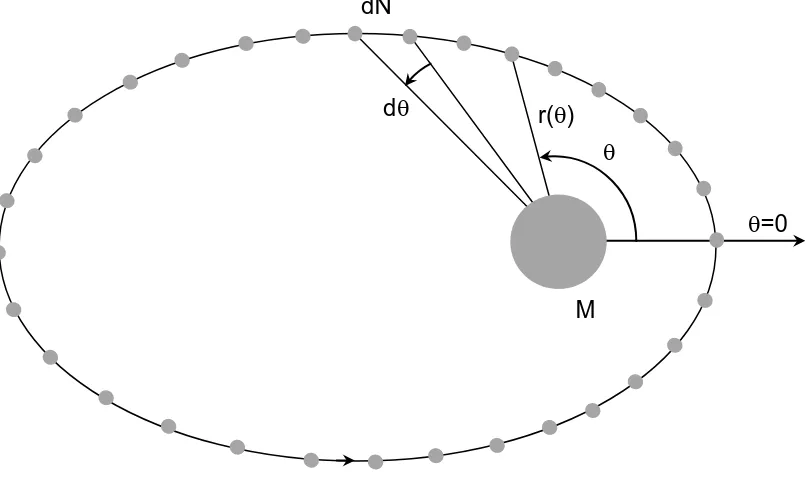
A single elliptical orbit of semi-major a and eccentricity e will now be considered, as shown
in Fig. 1, with the location of each node define by its true anomaly θ. A large number N of
∗Professor, Advanced Space Concepts Laboratory, Department of Mechanical and Aerospace Engineering,
colin.mcinnes@strath.ac.uk
nodes will be assumed to move along the elliptical orbit with local number density n
( )
θ,tdefined such that n
( )
θ,t dθ represents the number of nodes dN in the range(
θ,θ+dθ)
of theelliptical orbit at time t. The local angular velocity of each node dθ dt=ω
( )
θ is then defined by the dynamics of the two-body problem.The rate of change of the number of nodes in the constellation can be determined from
the flux of nodes at the boundaries θ =0 and θ =2π so that
( ) ( ) ( ) ( ) ( )
n t t n t t dt t dN , 2 , 2 , 0 ,0 ω − π ω π
= (1)
which can then be written as
( )
(
( ) ( )
)
∫
∂ ∂ − = π θ θ ω θ θ 2 0,t d n
dt t dN
(2)
The total number of nodes at time t can be determined by integrating the local density around
the elliptical ring such that
( )
=∫
( )
π θ θ 2 0,t d n t
N (3)
which is assumed to be constant. Therefore, combing Eq. (2) and Eq. (3) a continuity equation
is formed defined by
( )
(
( ) ( )
)
0 , , = ∂ ∂ + ∂∂ θ ωθ
θ θ t n t t n (4)
which represents a conservation law for the total number of nodes [8]. The solution to this
partial differential equation requires suitable boundary conditions, such as the initial value
problem posed by the initial distribution of nodes n
( )
θ,0 to obtain the number density ofThe local orbital angular velocity at some true anomaly θ along the elliptical ring can be determined from the conservation of angular momentum h such that r
( ) ( )
θ 2ωθ =h, where the local orbit radius is defined by r( )
θ =a(
1−e2)
(
1+ecosθ)
. The local angular velocity along the elliptical ring is then given by( ) (
)
2cos
1 θ
η θ
ω = +e (5)
where η=h a2
(
1−e2)
2. The continuity equation can now be solved using the method of characteristics [9] to provide a general solution n( )
θ,t for an arbitrary initial value problemdefined by n
( )
θ,0 , although it will later be assumed that the orbit eccentricity e is small.III. General solution to the continuity equation
Before solving the time-dependant continuity equation, a steady-state solution can be found
by requiring ∂n
( )
θ,t ∂t=0, so that the number density is a function of true anomaly only.Then, it can be seen from Eq. (4) that n
( ) ( )
θ ωθ is a conserved quantity, representing the fluxof nodes through an arbitrary point on the elliptical ring, with n
( )
θ inversely proportional to( )
θω as expected. If the number density is selected such that n
( )
0 =1 (at θ =0), then fromEq. (5) it can be seen that
( )
(
)
(
)
22
cos 1
1
θ θ
e e n
+ +
= (6)
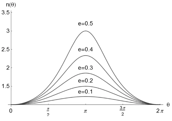
With this distribution of nodes the pattern formed by the constellation is invariant with time.
This is an exact solution of the continuity equation valid for all values of eccentricity e<1.
Such an initial distribution can be used in the design of an elliptical constellation which
requires a time invariant pattern. It can be seen from Eq. (7) that the number density at
apocenter is enhanced such that n
( ) ( ) (
π n0 =(
1+e) (
1−e)
)
2. The steady-state density functionis shown in Fig.2 as a function of eccentricity. For small eccentricities, n
( )
π ≈1+4e so thatthe apocenter density is enhanced by a factor of order 4e relative to the pericenter density. As
expected, the nodes cluster at apocenter corresponding to the minimum of the orbital angular
In order to now solve the full time-dependant continuity equation for the number
density n
( )
θ,t with arbitrary initial data n( )
θ,0 , Eq. (4) can be written as( ) ( ) ( ) ( ) ( )
θ θ ω θ θ θ θ ω θ d d t n t n t t n , , , − = ∂ ∂ + ∂ ∂ (7)Then, using the method of characteristics [9], the partial differential equation defined by Eq.
(7) can be written as two ordinary differential equations such that
( )
θ ω θ = dt d (8a)( )
( )
( ) ( )
n t d d d t dn , 1 , θ θ θ ω θ ω θθ =−
(8b)
where the partial differential equation is transformed into an ordinary differential equation
along the characteristic curves. In order to proceed with the analysis and obtain an explicit
closed-form solution, it is necessary to assume a small eccentricity for the ring, although an
implicit solution valid for high eccentricity is outlined in Appendix A. From Eq. (5) it can
then be seen that
( )
(
( )
2)
cos 2
1+ e +Oe
≈η θ
θ
ω (9)
and so
( )
η θθ θ ω sin 2e d d −
= (10)
The characteristics of the problem can now be obtained from Eq. (8a) and Eq. (9) as
for some arbitrary constant of integration C. This relation then integrates directly to
( )
(
e)
t C( )
t e , 2 tan 4 1 tan 4 12 1 2
2 − θ −η = θ
−
−
(12)
which is a essentially an approximate form of Kepler’s equation, relating true anomaly and
time in an explicit fashion. From Eq. (8b) and Eqs. (9) and (10), the number density n
( )
θ,tcan then be obtained from
( )
( )
t n e e d t dn , cos 2 1 sin 2 , θ θ θ θ θ += (13)
which again integrates directly to yield
( )
(
n t)
ln(
e)
(
C( )
t)
ln θ, =− 1+2 cosθ +Ψ θ, (14)
where Ψ
(
C( )
θ,t)
is some arbitrary function of the characteristic equation, to be determinedfrom the initial distribution of nodes n
( )
θ,0 . The general solution for the number density( )
tnθ, is finally obtained as
( )
(
( )
)
θ θ θ cos 2 1 , , e t C t n + Φ= (15)
where Φ
(
C( )
θ,t)
=exp(
Ψ(
C( )
θ,t)
)
. In order to proceed, initial data n( )
θ,0 must be providedto determine the functional form of Φ
(
C( )
θ,t)
, as will be seen in Section IV.Lastly, if a ring of uniform number density is required such that n
( )
θ,t =n, and so( )
, ∂ =0∂nθ t t and ∂n
( )
θ,t ∂θ =0, then from Eq. (7) it can be seen that( )
0 = − θ θ ω d dn (16)
be seen that a varying orbital angular momentum is required such that
(
)
2cos 1 θ ω η e + = (17)
which would require the use of continuous low thrust propulsion. Fixed spacing between
nodes is therefore possible on an elliptical ring, but with the added complexity of active
control.
IV. Closed-form solution for an initially uniform ring
As an example initial value problem, initial data n
( )
θ,0 =1 will be defined so that there is aninitially uniform distribution of nodes around the elliptical ring at t=0. From Eq. (3) the total
number N of nodes is then 2π. Since the local orbital angular velocity varies around the elliptical ring, the initially uniform distribution of nodes will evolve with time to form a
periodic pattern, with density enhancements at apocenter where the nodes naturally cluster
together. Using the initial data n
( )
θ,0 =1, from Eq. (15) it can be seen that( )
(
( )
)
1 cos 2 1 0 , 0 , = + Φ = θ θ θ e C n (18)The corresponding characteristic curves are then obtained from Eq. (12) as
( )
tan(
1 4 tan( )
2)
41 2 0
, 1 2
2 θ θ e e C − − = − (19)
In order to determine the functional form of the arbitrary function of the characteristic
( )
(
Cθ,t)
Φ , a new variable z =C
( )
θ,0 can be defined as( )
(
1 4 tan 2)
tan 4 1
2 1 2
2 e θ
e
z −
−
= −
(20)
− − = − z e e 2 4 1 tan 4 1 1 tan 2 2 2 1 θ (21)
Therefore, from Eq. (18) the arbitrary function Φ
(
C( )
θ,t)
can be obtained as( )
− − + = Φ − z e e e z 2 4 1 tan 4 1 1 tan 2 cos 2 1 2 2 1 (22)This function is unique to the initial data n
( )
θ,0 =1 and is selected to satisfy the boundaryconditions of the initial value problem. Now, substituting for z=C
( )
θ,t from Eq. (12), theclosed-form solution for the number density n
( )
θ,t with initial data n( )
θ,0 =1 is obtained as( )
( )
(
)
θ η θ θ cos 2 1 2 4 1 2 tan 4 1 tan tan 4 1 1 tan 2 cos 2 1 , 2 2 1 2 1 e t e e e e t n + − − − − + = − − (23)which again clearly satisfies the boundary condition n
( )
θ,0 =1. This solutions now represents the evolution of the initially uniform distribution of nodes as a function of both true anomalyand time.
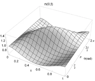
Being a function of both variables, Eq. (23) therefore represents a surface n
( )
θ,t , as shown in Fig. 3, where canonical units are used with µ=a=1 and the time variable re-scaledsuch that a complete orbital period occurs across the range 0≤t≤1. It can be seen from Fig. 3 that the initially uniform distribution of nodes is compressed close to apocenter,
corresponding to the minimum of orbital angular velocity around the elliptical ring, and are
rarefied at pericenter corresponding to the maximum of orbital angular velocity. The pattern
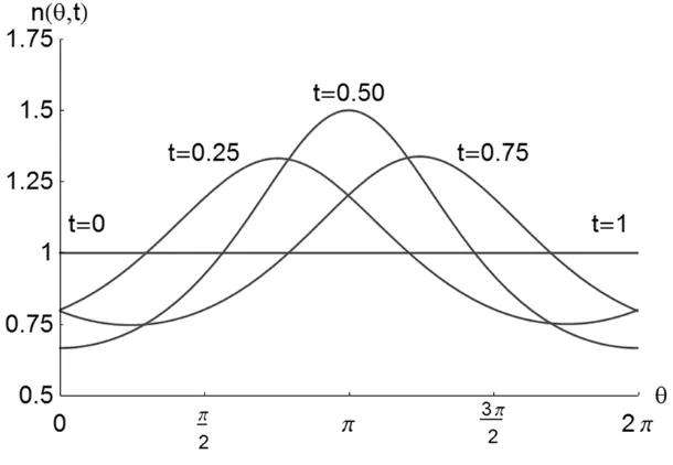
formed by the nodes is therefore wave-like and circulates around the elliptical ring. The
propagation of the wave-like pattern can be seen in Fig. 4 for a series of time steps. The wave
forms at pericenter and circulates to apocenter where the number density is maximum, and
then to pericenter repeating every orbit period. Clearly this is not a mechanical density wave,
since there is no physical interaction between the nodes, but is does represent a periodic
pattern, as opposed to the time invariant pattern defined by Eq. (6), could be used to provide
enhanced coverage by phasing the peaks in number density to occur at target locations on the
constellation ground track.
The solution provided by Eq. (23) can also be expanded in eccentricity, since the
closed form solution assumes small eccentricity, to obtain a simplified solution of the form
( )
(
(
1(
(
( )
)
)
)
) ( )
22 tan
tan 2 cos cos
2 1
,t e t Oe
nθ = − θ − − η − θ + (24)
which again represents a wave-like pattern propagating around the elliptical ring. Considering
the time variation of the density observed at the pericenter and apocenter of the ring it can be
seen that
( )
(
( )
)
( )
2cos 1 2 1 ,
0t e t Oe
n = − − η + (25a)
( )
(
( )
)
( )
2cos 1 2 1
,t e t Oe
nπ = + − η + (25b)
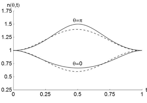
so that the density at pericenter therefore falls by ∆n≈−2e, whilst the density at apocenter is enhanced by ∆n≈+2e as expected. The observed variation in number density at pericenter
( )
tn0, and apocenter n
( )
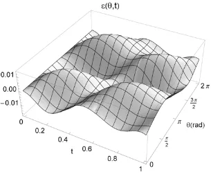
π,t is shown in Fig. 5 along with the approximation defined by Eq. (25).Finally, in order to assess the accuracy of the closed-form solution presented in Eq.
(23), a comparison can be made with a numerical solution of the continuity equation defined
by Eq. (4) for initial number density n
( )
θ,0 =1. The partial differential equation can be solved numerically using the method of lines, while enforcing the periodic boundary condition( ) (
t n t)
n0, = 2π, , in addition to the initial data n
( )
θ,0 =1. The analytic solution nA( )
θ,t can becompared with the numerical solution nN
( )
θ,t through a relative error function( )
θ,t 1 nA( ) ( )
θ,t nN θ,tε = − , as shown in Fig. 6. It can be seen that for the orbit eccentricity
e=0.1 considered above, the relative error is modest with ε
( )
θ,t ≈0.01.V. Conclusions
been presented using a continuum approach and deriving a continuity equation for the number
density of nodes on the ring. For small eccentricities, the continuity equation can be solved
explicitly in closed-form for some initial distribution of nodes. The resulting solution
represents the evolution of an initial distribution of nodes as a function of both time and true
anomaly and exhibits a wave-like pattern which propagates around the elliptical ring. The
nodes are compressed in number density close to apocenter, corresponding to the minimum of
orbital angular velocity around the elliptical ring, and rarefied at pericenter corresponding to
the maximum of orbital angular velocity.
Appendix A: Implicit solution valid for high eccentricity
The closed-form solution presented in Eq. (23) provides an explicit solution for the number
density of nodes n
( )
θ,t as a function of both polar angle and time. Such an explicit solution ispossible since the small eccentricity approximation used allows Eq. (20) to be inverted,
essentially allowing an explicit mapping between polar angle and time. However, it is possible
to generate an implicit solution for the number density of nodes valid for high eccentricity.
Without the small eccentricity approximation Eq. (10) yields
( )
η θ(
θ)
θ θ ω cos 1 sin
2e e
d
d =− +
(A1)
which can be integrated to obtain an implicit relationship between polar angle and time as
(
)
( )
(
)
(
)
t C( )
te e e e e e , cos 1 1 sin 2 tan 1 1 tan 2 1 1 2 1 2 3
2 θ η θ
θ
θ − =
+ − − + − − − (A2)
The number density n
( )
θ,t can then be found from Eq. (8b) by integrating( )
(
( )
)
(
)
2cos 1
, ,
θ θ θ
e t C t
n
+ Φ
= (A4)
which again is valid for high eccentricity. For some initial value problem, for example with
( )
θ,0 =1n , the arbitrary function Φ
(
C( )
θ,t)
can again be obtained from the initial data. However, since Eq. (A2) is an implicit relationship, evaluation of this function requiresnumerical iteration, akin to solving Kepler’s equation at each point in the evaluation of the
solution. To this end it can be shown that Eq. (A2) can be written as a function of eccentric
anomaly E such that
(
2)
3 2( )
sin
, 1
E e E
t C t
e
η θ
− − =
− (A5)
This implicit relation can again be solved using standard numerical methods to obtain the
number density of nodes n
( )
θ,t as a function of both polar angle and time.Acknowledgments
This work was supported by European Research Council grant 227571 (VISIONSPACE).
References
[1] Driam, J.E., Cefola, P., and Castrel, D., “Elliptical Orbit Constellations - A New Paradigm
for Higher Efficiency in Space Systems?”, IEEE Aerospace Conference Proceedings, 18-25
March 2000, Big Sky, Montana.
[2] Wertz, J.R., “Coverage, Responsiveness and Accessibility for Various Responsive Orbits,”
AIAA RS3-2005-2001, 3rd Responsive Space Conference, Los Angeles, 25-28 April 2005.
[3] Janson, S.W., "Silicon Satellites: Picosats, Nanosats and Microsats,"inProceedings of the
International Conference on Integrated Micro/Nanotechnology for Space Applications, The
Aerospace Press, El Segundo, CA, and AIAA, Reston, VA, Houston, 30 October - 3
November 1995.
[4] Barnhart, D. J., Vladimirova, T. and Sweeting, M. N., “Very-Small-Satellite Design for
Distributed Space Missions,” Journal of Spacecraft and Rockets, Vol. 44, No. 6, 2007, pp.
[5] Atchison, J. A. and Peck, M. A., “A Passive, Sun-Pointing, Millimeter-Scale Solar Sail,”
Acta Astronautica, Vol. 67, No. 1-2, 2009, pp. 108-121.
[6] McInnes, C.R., "An Analytical Model for the Catastrophic Production of Orbital Debris,"
ESA Journal, Vol. 17, No. 4, 1993, pp. 293-305.
[7] McInnes, C.R., “A Simple Analytic Model of the Long Term Evolution of Nanosatellite
Constellations,” Journal of Guidance, Control and Dynamics, Vol. 23, 2000, No. 2, pp.
332-338.
[8] Acheson, D.J., Elementary Fluid Dynamics, Clarendon Press, Oxford, 1990, pp. 2-7.
Figure Captions
Figure 1. Ring of nodes of number density n
( )
θ,t on an elliptical orbit.Figure 2. Steady-state number density n
( )
θ for eccentricity e= 0.1, 0.2, 0.3, 0.4, 0.5.Figure 3. Density n
( )
θ,t for an initially uniform distribution of nodes n( )
θ,0 =1 on anelliptical orbit of eccentricity e=0.1 for 0≤θ 2π and 0≤t≤1.
Figure 4. Density waves obtained on an elliptical orbit of eccentricity e=0.1 from an initially
uniform distribution of nodes n
( )
θ,0 =1 for time steps t= 0, 0.25, 0.5, 0.75, 1.Figure 5. Observed number density for an initially uniform distribution of nodes n
( )
θ,0 =1 onan elliptical orbit of eccentricity e=0.1 as a function of time t at perigee n
( )
0,t and apogee( )
tnπ, (_____ analytic solution, - - - approximation).
Figure 6. Comparison of analytical and numerical solutions to the continuity illustrating the
Figure 1
θ
θ=0
M dN
Figure 2