Volume 78, Number 266, April 2009, Pages 789–814 S 0025-5718(08)02172-8
Article electronically published on November 24, 2008
DERIVING A NEW DOMAIN DECOMPOSITION METHOD FOR THE STOKES EQUATIONS
USING THE SMITH FACTORIZATION
VICTORITA DOLEAN, FR ´ED ´ERIC NATAF, AND GERD RAPIN
Abstract. In this paper the Smith factorization is used systematically to derive a new domain decomposition method for the Stokes problem. In two dimensions the key idea is the transformation of the Stokes problem into a scalar bi-harmonic problem. We show, how a proposed domain decomposi-tion method for the bi-harmonic problem leads to a domain decomposidecomposi-tion method for the Stokes equations which inherits the convergence behavior of the scalar problem. Thus, it is sufficient to study the convergence of the scalar algorithm. The same procedure can also be applied to the three-dimensional Stokes problem.
As transmission conditions for the resulting domain decomposition method of the Stokes problem we obtain natural boundary conditions. Therefore it can be implemented easily.
A Fourier analysis and some numerical experiments show very fast conver-gence of the proposed algorithm. Our algorithm shows a more robust behavior than Neumann-Neumann or FETI type methods.
1. Introduction
The last decade has shown, that Neumann-Neumann type algorithms, FETI, and BDDC methods are very efficient domain decomposition methods. Most of the early theoretical and numerical work has been carried out for scalar symmetric positive definite second order problems; see for example [6], [13]–[15], [23]. Then, the method was extended to other problems, like the advection-diffusion equations [1, 7], plate and shell problems [27] or the Stokes equations [26, 22].
In the literature one can also find other preconditioners for the Schur comple-ment of the Stokes equations (cf. [2, 26]). Moreover, there exist some Schwarz-type algorithms for non-overlapping decompositions (cf. [16, 19, 20, 24]). A more com-plete list of domain decomposition methods for the Stokes equations can be found in [22, 28]. Also FETI [11] and BDDC methods [12] are applied to the Stokes problem with success.
Our work is motivated by the fact that in some sense the domain decomposition methods for Stokes are less optimal than the domain decomposition methods for scalar problems. Indeed, in the case of two subdomains consisting of the two half-planes it is well known that the Neumann-Neumann preconditioner is an exact preconditioner for the Schur complement equation for scalar equations like the Laplace problem (cf. [23]). A preconditioner is calledexact, if the preconditioned
Received by the editor October 17, 2006 and, in revised form, October 29, 2007. 2000Mathematics Subject Classification. 65-xx .
c
operator simplifies to the identity. Unfortunately, this does not hold in the vector case. It is shown in [18] that the standard Neumann-Neumann preconditioner for the Stokes equations does not possess this property.
Our aim in this paper is the construction of a method, which preserves this property. Thus, one can expect a very fast convergence for such an algorithm; and indeed, the numerical results clearly support our approach. This paper explains the ideas of [4] in more detail. For an application to the compressible Euler equations see [3].
Let us give a short outline of the paper. In Section 2 we introduce the Stokes equations. Concentrating on the two-dimensional case, these equations are trans-formed into a bi-harmonic operator with the help of the Smith factorization. Then, in Section 3 we first introduce an iterative domain decomposition method for the bi-harmonic equations and we show how it can be used for the Stokes equations. Moreover, in Section 4 we discuss briefly, how this approach can be extended to the linearized Navier-Stokes equations (Oseen equations). In the case of two sub-domains we were able to derive an algorithm which converges independently of the Reynolds number in two iterations. Most likely, ongoing research will show that we will retrieve this behavior for more general decompositions. Then, in Section 5 the algorithm is extended to the three-dimensional Stokes problem. A finite volume discretization is discussed in Section 6. Section 7 is dedicated to numerical results for the two-dimensional Stokes problem. Finally, we give some concluding remarks.
2. Equivalence between the Stokes equations and the bi-harmonic problem
In this section we show the equivalence between the Stokes system and a fourth order scalar problem (the bi-harmonic problem) by means of the Smith factoriza-tion. This is motivated by the fact that scalar problems are easier to manipulate and the construction of new algorithms is more intuitive. Additionally, the existing theory of scalar problems can be used.
2.1. Stokes equations. We consider the stationary Stokes problem in a bounded
domain Ω ⊂Rd, d = 2,3. The Stokes equations are given by a velocity u and a pressurepsatisfying
−ν∆u+∇p+cu = f in Ω,
∇ ·u = 0 in Ω,
and some boundary conditions on∂Ω. The Stokes problem is a simple model for incompressible flows. The right hand side of f = (f1, . . . , fd)T ∈ [L2(Ω)]d is a
source term, ν is the viscosity and c ≥0 is a constant reaction coefficient. Very oftencstems from an implicit time discretization and thencis given by the inverse of the time step size.
In the following we denote the d-dimensional Stokes operator by Sd(v, q) :=
(−ν∆v+cv+∇q,∇ ·v).
2.2. Smith factorization. Now we show that the Stokes problem can be
trans-formed into a scalar fourth order problem using the Smith factorization. We recall the Smith factorization of a matrix with polynomial entries ([29], Theorem 1.4):
Theorem 2.1. Let n be an positive integer and A an invertible n×n matrix
there exist matrices E, D and F with polynomial entries satisfying the following properties:
• det(E)anddet(F)are constants,
• Dis a diagonal matrix uniquely determined up to a multiplicative constant,
• A=EDF.
Here E andF are matrices, which operate on the rows, respectively, columns. The entries of the diagonal matrixD= (dij(λ))are given bydii=φi/φi−1, whereφi is the greatest common divisor of the determinants of all i×i submatrices ofA and φ0= 1.
The Smith factorization is a classical tool in computer algebra and in control of ordinary differential equations. Since its use in scientific computing is rather new, we give here a few comments:
• Smith was an English mathematician of the end of the nineteenth century. He worked in number theory and considered the problem of factorizing matrices with integer entries. We give here the polynomial version of his theorem in the special case where the matrix A is square and invertible but the result is more general and applies as well when the matrix A is rectangular.
• One interesting fact of the theorem is the following. By Cramer’s formula, the inverse ofA is in general a matrix with rational entries. By the Smith factorization, we have A−1 =F−1D−1E−1. Since det(E) and det(F) are constants, the inverse ofE andF are still matrices with polynomial entries in λ. The rational part of the inverse of A is thus in D−1 which is an intrinsic diagonal matrix.
• The proof of the theorem is constructive and gives an algorithm for comput-ing matricesE, D andF. As stated in the theorem, matrixD is intrinsic but matricesE andF are not unique.
• In the sequel, we write the Stokes equations as a matrix with partial differ-ential operator entries applied to the unknown velocity and pressure fields. The direction normal to the interface of the subdomains is particularized and denoted by∂x. Each partial differential operator is then considered as
a polynomial in the “variable∂x” (e.g. λ is related to∂x and λ2 to ∂xx).
It is then possible to apply the Smith factorization; see below.
Application to the two-dimensional Stokes problem. The Smith
factoriza-tion is applied to the following model problem in the whole planeR2, Sd(u, p) = g inR2,
(2.1)
|u(x)| → 0 for|x| → ∞
(2.2)
with the right hand sideg= (f1, f2,0)T. Moreover, it is assumed, that the coeffi-cientsc, νare constants.
We start with the two-dimensional case. The spatial coefficients are denoted by
equation (2.1) yields ˆS2(ˆu,pˆ) = ˆgwith ˆu= (ˆu,vˆ) and
(2.3) S2(ˆˆ u,pˆ) =
⎛
⎝ −ν(∂xx−k
2) +c 0 ∂
x
0 −ν(∂xx−k2) +c ik
∂x ik 0
⎞ ⎠
⎛ ⎝ uvˆˆ
ˆ
p ⎞ ⎠.
Considering ˆS2as a matrix with polynomial entries with respect to∂x, we perform
fork= 0 the Smith factorization. We obtain (2.4) S2ˆ = ˆE2Dˆ2Fˆ2 with
ˆ
D2=
⎛
⎝ 10 01 00 0 0 (∂xx−k2) ˆL2
⎞
⎠, Fˆ2=
⎛ ⎝ νk
2+c νik∂
x ∂x
0 L2ˆ ik
0 1 0
⎞ ⎠
and
ˆ
E2= ˆT2−1
⎛ ⎝ ik
ˆ
L2 ν∂xxx −ν∂x
0 Tˆ2 0
ik∂x −∂xx 1
⎞ ⎠
where T2 is a differential operator in they-direction whose symbol isik(νk2+c). Moreover, ˆL2:=ν(−∂xx+k2) +c is the Fourier transform ofL2:=−ν∆ +c. Remark 2.2. Using this factorization, problem (2.1) can be written as
(2.5) Dˆ2wˆ= ˆE2−1ˆg, wˆ:= ( ˆw1,wˆ2,wˆ3)T := ˆF2(ˆu,pˆ)T. From (2.5) we get ˆw1= ( ˆE2−1ˆg)1 and ˆw2= ( ˆE2−1gˆ)2. Noticing that
ˆ
w3=
ˆ
F2(ˆu,pˆ)T
3 = ˆv
the previous equation yields, after applying an inverse Fourier transform, ∆(−ν∆ +c)v=Fy−1
( ˆE−21gˆ)3
.
Since the matrices ˆE2 and ˆF2 have a determinant which is a non-zero number (i.e. a polynomial of degree zero), the entries of their inverses are still polynomial in
∂x. Thus, applying ˆE2−1to the right hand side ˆg, amounts to taking derivatives of ˆ
g and making linear combinations of them. If the planeRis split into subdomains
R−×R and R+×R, the application of ˆE−1
2 and ˆF− 1
2 to a vector can be done for each subdomain independently. No communication between the subdomains is necessary.
3. A new algorithm for the Stokes equations
Our goal is to write for the Stokes equations on the whole plane divided into two half-planes an algorithm converging in two iterations. Section 2.2 shows that the design of an algorithm for the fourth order operatorB := ∆L2 = ∆(−ν∆ +c) is a key ingredient for this task. Therefore, we derive an algorithm for the operator B and then, via the Smith factorization, we recast it in a new algorithm for the Stokes system.
3.1. An optimal algorithm for the scalar fourth order operator. We
con-sider the following problem: Findφ:R2→Rsuch that (3.1) B(φ) =gin R2, |φ(x)| →0 for|x| → ∞
where g is a given right hand side. The domain Ω is decomposed into two half-planes Ω1 =R−×Rand Ω2=R+×R. Let the interface {0} ×R be denoted by Γ and (ni)i=1,2 be the outward normal of (Ωi)i=1,2. The algorithm, we propose, is
given as follows:
Algorithm 3.1. We choose the initial values φ0
1 and φ02 such that φ01 =φ02 and L2φ0
1=L2φ02 onΓ. We obtain(φ
n+1
i )i=1,2from(φni)i=1,2by the following iterative
procedure:
Correction step. We compute the corrections ( ˜φni+1)i=1,2 as solutions of the
homogeneous local problems
(3.2) ⎧ ⎪ ⎪ ⎪ ⎪ ⎪ ⎪ ⎪ ⎪ ⎨ ⎪ ⎪ ⎪ ⎪ ⎪ ⎪ ⎪ ⎪ ⎩
Bφ˜n+1
1 = 0in Ω1, lim
|x|→∞|
˜
φn1+1|= 0, ∂φ˜n1+1
∂n1
=γ1n onΓ, ∂L2φ˜n1+1
∂n1
=γn2 onΓ,
⎧ ⎪ ⎪ ⎪ ⎪ ⎪ ⎪ ⎪ ⎪ ⎨ ⎪ ⎪ ⎪ ⎪ ⎪ ⎪ ⎪ ⎪ ⎩
Bφ˜n+1
2 = 0 inΩ2, lim
|x|→∞|
˜
φn2+1|= 0, ∂φ˜n2+1
∂n2
=γn1 onΓ, ∂L2φ˜n2+1
∂n2
=γ2n onΓ,
whereγn
1 =− 1 2
∂φn
1
∂n1 +∂φ
n
2
∂n2
andγn
2 =− 1 2
∂L2φn
1
∂n1
+∂L2φ
n
2
∂n2
.
Updating step. We update(φni+1)i=1,2 by solving the local problems
(3.3) ⎧ ⎪ ⎪ ⎪ ⎪ ⎨ ⎪ ⎪ ⎪ ⎪ ⎩
Bφn1+1=g in Ω1,
lim
|x|→∞|
φn1+1|= 0, φn1+1=φn1+δ
n+1 1 on Γ, L2φn1+1=L2φ1n+δ2n+1 on Γ,
⎧ ⎪ ⎪ ⎪ ⎪ ⎨ ⎪ ⎪ ⎪ ⎪ ⎩
Bφn2+1 =g in Ω2,
lim
|x|→∞|
φn2+1|= 0, φn2+1=φn2+δ
n+1 1 on Γ, L2φn2+1=L2φ2n+δn2+1 on Γ,
whereδn1+1=1 2( ˜φ
n+1 1 + ˜φ
n+1 2 )andδ
n+1 2 =
1 2(L2
˜
φn1+1+L2φ˜n2+1).
This algorithm has the proposed remarkable property. Formally we can show:
Proposition 3.2. Algorithm 3.1 converges in two iterations.
Proof. The equations and the algorithm are linear. It suffices to prove convergence to zero of the above algorithm wheng≡0. We make use of the Fourier transform in the y direction. First of all, as φ0
we obtain the same properties forφ11 and φ12. Then, note that at each step of the algorithmφni satisfies the homogeneous equation in each subdomain
(3.4) Bˆφˆni(x, k) = (∂xx−k2)(−ν(∂xx−k2) +c) ˆφni(x, k) = 0.
For each k ∈ R, (3.4) is a fourth order ordinary differential equation in x. The solution in each domain tends to 0 as |x| tends to ∞. Just in order to simplify computations we assumec >0. See [18] for the casec= 0. Therefore, we get
(3.5) φˆ
n
1(x, k) =α
n
1(k)e|
k|x+βn
1(k)e
λ(k)x,
ˆ
φn2(x, k) =αn2(k)e−|k|x+β2n(k)e−λ(k)x
withλ(k) =c/ν+k2. The first continuity relationL2φ1
1=L2φ12on the interface Γ leads toα1
1(k) =α12(k) as ˆ
L2φˆ1
i(0, k) = (−ν(∂xx−k2) +c) ˆφ1i(0, k)
= −ν(−k2+λ2(k))β1
i(k) +c(α1i(k) +βi1(k)) =cα1i(k), i= 1,2,
and from φ1
1 = φ12 on Γ we finally get β11(k) = β12(k). Therefore, we can omit the subscript indicating the number of the subdomain in αand β. Then, we can computeγ1
1,γ21used by thecorrection step(3.2):
γ1
1=−(α1(k)|k|+β1(k)λ(k)),
γ1
2=−α1(k)|k|c.
A direct computation shows that the solutions of the correction stepφ˜2i, i= 1,2, whose expressions are of the form (3.5) are given by
˜
φ2
1(x, k) =−α
1(k)e|k|x−β1(k)eλ(k)x,
˜
φ2
2(x, k) =−α
1(k)e−|k|x−β1(k)e−λ(k)x.
Inserting this into (3.3) shows that the right hand side of the boundary conditions are zero. Since we assumedg≡0, this shows that ˆφ2i = 0 fori= 1,2.
3.2. From the fourth order operator B to the Stokes system. After
hav-ing found an optimal algorithm which converges in two steps for the fourth order operator Bproblem, we focus on the Stokes system (2.1)-(2.2) by translating this algorithm into an algorithm for the Stokes system. It suffices to replace the opera-torBby the Stokes system andφby the last component (F2(u, p)T)3of the vector F2(u, p)T in the boundary conditions, by using formula (2.5).
The algorithm reads:
Algorithm 3.3. We choose the initial values(u0
1, p01)and(u02, p02)such that (F2(u01, p01)T)3= (F2(u02, p02)T)3
and
L2(F2(u01, p01)T)3=L2(F2(u02, p02)T)3
onΓ. We compute((uni+1, pni+1))i=1,2from((uni, pni))i=1,2by the following iterative
procedure:
of the homogeneous local problems: (3.6)⎧ ⎪ ⎪ ⎪ ⎪ ⎪ ⎪ ⎪ ⎪ ⎨ ⎪ ⎪ ⎪ ⎪ ⎪ ⎪ ⎪ ⎪ ⎩
S2(u˜n1+1,p˜n1+1) = 0 inΩ1, lim
|x|→∞| ˜
un1+1|= 0, ∂(F2(u˜n1+1,p˜
n+1 1 )
T)
3
∂n1
=γ1n onΓ,
∂L2(F2(u˜n1+1,p˜
n+1 1 )T)3
∂n1
=γn2 onΓ, ⎧ ⎪ ⎪ ⎪ ⎪ ⎪ ⎪ ⎪ ⎪ ⎨ ⎪ ⎪ ⎪ ⎪ ⎪ ⎪ ⎪ ⎪ ⎩
S2(u˜n2+1,p˜n2+1) = 0 inΩ2, lim
|x|→∞| ˜
un2+1|= 0, ∂(F2(u˜n2+1,p˜
n+1 2 )
T)
3
∂n2
=γ1n onΓ,
∂L2(F2(u˜n2+1,p˜
n+1 2 )T)3
∂n2
=γ2n onΓ, where
γn
1 =− 1 2
∂(F2(un1, pn1)T)3
∂n1
+∂(F2(u
n
2, pn2)T)3
∂n2
,
γn
2 =− 1 2
∂L2(F2(un1, pn1)T)3
∂n1
+∂L2(F2(u
n
2, pn2)T)3
∂n2
.
Updating step. We update((uni+1, pin+1))i=1,2 by solving the local problems:
(3.7) ⎧ ⎪ ⎪ ⎪ ⎪ ⎨ ⎪ ⎪ ⎪ ⎪ ⎩
S2(uni+1, pin+1) =g inΩi,
lim
|x|→∞|u n+1
i |= 0,
(F2(uni+1, p n+1
i )
T)
3= (F2(uni, p n i)
T)
3+δ1n+1 on Γ, L2(F2(uni+1, pin+1)T)3=L2(F2(uni, pni)T)3+δ2n+1 on Γ, where
δn1+1=1 2[(F2(
u˜n+1 1 ,p˜
n+1 1 )
T)3+ (F2(u˜n+1 2 ,p˜
n+1 2 )
T)3],
δn2+1=1
2[L2(F2(
u˜n+1 1 ,p˜
n+1 1 )
T)3+L2(F2(u˜n+1 2 ,p˜
n+1 2 )
T)3].
This algorithm seems quite complex since it involves third order derivatives of the unknowns in the boundary conditions on (F2(u˜i,p˜i)T)3. Writingui = (ui, vi)
and using (F2(u˜i,p˜i)T)3 = ˜vi, it is possible to simplify it. By using the Stokes
equations in the subdomains, we can lower the degree of the derivatives in the boundary conditions. In order to ease the presentation in Algorithm 3.4 we do not mention that the solutions tend to zero as |x| → ∞. If we denote the k-th component of the unit outward normal vectorni of Ωi byni,k, we obtain for two
subdomains the following:
Algorithm 3.4. We choose the initial values(u01, v01, p01)and(u02, v20, p02)such that v10=v02 and
ν∂u
0 1
∂n1 −
p01n1,1=−
ν∂u
0 2
∂n2 −
p02n2,1
onΓ. We compute((uni+1, vin+1, pni+1))i=1,2from((uni, vni, pni))i=1,2by the following
iterative procedure:
Correction step. We compute the corrections ((˜uni+1,˜vin+1,p˜ni+1))i=1,2 as the
solution of the homogeneous local problems:
(3.8) ⎧ ⎪ ⎪ ⎨ ⎪ ⎪ ⎩
S2(˜un1+1,v˜1n+1,p˜n1+1) = 0inΩ1, ν∂˜v
n+1 1
∂n1
=γ1n onΓ,
˜
un1+1=γn
2,1 onΓ,
⎧ ⎪ ⎪ ⎨ ⎪ ⎪ ⎩
S2(˜un2+1,˜v2n+1,p˜n2+1) = 0 inΩ2, ν∂˜v
n+1 2
∂n2
=γ1n onΓ,
˜
un2+1=γn
whereγn
1 =− 1 2 ν∂v n 1
∂n1 +ν∂v
n
2
∂n2
andγn
2,i= (−1)i
1 2(u
n
1−u
n
2).
Updating step. We update((uni+1, vin+1, pni+1))i=1,2by solving the local problems:
(3.9) ⎧ ⎪ ⎪ ⎪ ⎨ ⎪ ⎪ ⎪ ⎩
S2(uni+1, vin+1, pin+1) =g inΩi, ν∂u
n+1
i ∂ni
−pni+1ni,1=ν
∂un i ∂ni
−pnini,1+δijn+1 onΓ, vin+1=vin+1
2(˜v
n
1 + ˜v
n
2) onΓ,
whereδnij+1=1 2
ν∂u˜
n+1
i ∂ni
−p˜ni+1ni,1
−1 2
ν∂u˜
n+1
j ∂nj
−p˜nj+1nj,1
andj= 3−i.
Lemma 3.5. Consider the model caseΩ =R2,Ω1 =R−×Rand Ω2 =R+×R.
We assume that all variables vanish at infinity. Then, the Algorithms 3.3and 3.4
are equivalent.
Proof. First, notice (F2(u˜ni,p˜ni)T)3 = ˜vni and (F2(uni, pni)T)3 =vni. Thus, the first
interface conditions of (3.6), respectively, (3.7) are obviously the same as the first interface conditions of (3.8), respectively, the second one of (3.9).
To prove the complete equivalence between these algorithms, we start with the local problems in Ω1by transforming the second interface condition of the correction step (3.6):
∂xL2˜vn1+1=− 1 2∂x(L2v
n
1 − L2v
n
2) on Γ. Using the second equation of the Stokes system,
L2(F2(uni, pin)T)3= (−ν∆ +c)vni =∂ypni +f2, i= 1,2, we obtain
∂x(−∂yp˜n1+1) =− 1
2∂x((−∂yp
n
1+f2)−(−∂ypn2+f2)), =−1
2∂y(−∂xp
n
1 +∂xpn2) on Γ.
Interchanging the partial derivatives and using the first equation of the Stokes system and the fact that all functions vanish at infinity, by integrating with respect toy we get
∂y(L2u˜n1+1) =− 1
2∂y(L2u
n
1 − L2u
n
2) on Γ⇔ L2u˜n1+1=−1
2(L2u
n
1 − L2u
n
2) on Γ. (3.10)
Differentiating the first interface condition (3.6) with respect to y and using the incompressibility constraint (∂yv˜in+1=−∂xu˜ni+1, i= 1,2) yields
(3.11) −ν∂xxu˜n1+1= 1 2ν∂xx(u
n
1−u
n
2) on Γ. We subtract (3.11) from (3.10). Thus, we obtain
(−ν∂yy+c)˜un1+1=− 1
2(−ν∂yy+c)(u
n
1−u
n
2) on Γ⇔ ˜
un1+1=−1 2(u
n
1−u
n
which is exactly the second transmission condition (3.8) of the correction step. Next, we consider the second interface condition of the updating step (3.7). Using again the second equation of the Stokes system we obtain:
∂ypn1+1=∂ypn1 + 1 2
∂yp˜n1+1+∂yp˜n2+1
on Γ⇔
pn1+1=pn1+1 2
˜
pn1+1+ ˜pn1+1 on Γ.
(3.12)
Of course, one could stop with boundary condition (3.12), but we will derive a more natural boundary condition. Therefore, we also use the second transmission condi-tion of (3.7) and mix both condicondi-tions. Differentiating the first interface condicondi-tion of (3.7) with respect toy gives
∂yv1n+1=∂yv1n+ 1 2∂y
˜
v1n+1+ ˜vn2+1 on Γ.
Now, using the incompressibility constraint yields (3.13) −ν∂xun1+1=−ν∂xun1−
1 2ν∂x
˜
un1+1+ ˜un2+1 on Γ.
Adding (3.12) and (3.13) we end up with −ν∂xun1+1+p
n+1
1 = −ν∂xun1 +p
n
1 +1
2
−ν∂xu˜n1+1+ ˜p
n+1 1
+1 2
−ν∂xu˜n2+1+ ˜p
n+1 2
,
which is exactly the first transmission condition (3.9) of the updating step. The reformulation of the initial conditions can be done analogously.
The same computations can be performed for subdomain Ω2.
Remark 3.6. The assumption that the pressure vanishes at infinity is artificial. If we only use that the derivatives ofpvanish, then the first interface condition of the updating step is determined only up to a constant. In practice, one could easily avoid this problem by providing an appropriate coarse space.
In order to write the resulting algorithm in an intrinsic form, we introduce the stressσi(u, p) for each subdomain Ω
i on the interface for a velocityu= (u, v), a
pressurepand the normal vectorni. If∂ni=∂x, we have the following formula in
cartesian coordinates:
σi(u, p) = (ν∂u ∂x−p,
ν
2(
∂v ∂x+
∂u ∂y)).
For any vector u its normal (resp. tangential) component on the interface is
uni = u·ni (resp. uτi = (I−ni⊗ni)u). We denote σ
i ni := σ
i
ni(ui, pi)·ni and
σi
τi := (I−ni⊗ni)σ
i as the normal and tangential parts ofσi, respectively.
Moreover, we notice that boundary conditions (3.8) are equivalent to conditions (3.14). Indeed, it suffices to differentiate w.r.t they direction the boundary condi-tion on the normal velocity in (3.8), multiply it by ν and add it to the boundary condition on the normal derivative of the tangential velocity in (3.8).
interface between subdomains Ωi and Ωj,i=j. The new algorithm for the Stokes
system reads:
Algorithm 3.7. Starting with an initial guess((u0
i, p0i))Ni=0 satisfyingu0i,τi=u 0
j,τj
andσi ni(u
0
i, p0i) =σ j nj(u
0
j, p0j)onΓij,∀i, j,i=j, thecorrection stepis expressed as follows for 1≤i≤N:
⎧ ⎪ ⎪ ⎪ ⎨ ⎪ ⎪ ⎪ ⎩
S2(˜uni+1,p˜ni+1) = 0 in Ωi,
˜
uni,+1n
i =−
1 2(u
n i,ni+u
n
j,nj) on Γij,
σiτ
i(
u˜n+1
i ,p˜ n+1
i ) =−
1 2(σ
i τi(u
n i,p˜
n i) +σ
j τj(u
n j,p˜
n
j)) onΓij.
(3.14)
followed by anupdating stepfor1≤i≤N:
(3.15) ⎧ ⎪ ⎪ ⎪ ⎪ ⎪ ⎨ ⎪ ⎪ ⎪ ⎪ ⎪ ⎩
S2(uni+1, pin+1) =g in Ωi,
uni,+1τ
i =u
n i,τi+
1 2(
u˜n+1
i,τi +
u˜n+1
j,τj) onΓij,
σnii(uni+1, pni+1) =σini(uni, pni),
+1 2(σ
i ni(˜u
n+1
i ,p˜ n+1
i ) +σ j nj(˜u
n+1
j ,p˜ n+1
j ))onΓij.
The boundary conditions in the correction step involve the normal velocity and the tangential stress, whereas in the updating step the tangential velocity and the normal stress are involved. As we will see in Section 5, in three dimensions the algorithm has the same definition.
Proposition 3.8. For a domain Ω = R2 divided into two non-overlapping
half-planes, Algorithms 3.3and 3.7are equivalent and both converge in two iterations. Proof. The equivalence of both algorithms has already been shown. The conver-gence in two steps of Algorithm 3.7 is obvious, since the algorithm was derived directly from Algorithm 3.3 which converges in two steps.
4. Extension to the Oseen equations
The next step is an extension of this technique to the Oseen equations
−ν∆u+b · ∇u+cu+∇p = f in Ω,
∇ ·u = 0 in Ω.
(4.1)
In comparison to the Stokes equations we have added the convective termb · ∇u. Now, the equation is no longer symmetric. Standard linearization techniques for the incompressible Navier-Stokes equations lead to the Oseen problem. Therefore, the efficient numerical solution of the Oseen problem is very important. The Oseen operator is given by
Od(u, p) =
−ν∆u+b · ∇u+cu+∇p,∇ ·u T
, d= 2,3.
the Smith factorization to the Fourier transform ofO2 (inydirection) yields ˆO2= ˆ
EO
2Dˆ2OFˆ2O. The diagonal matrix is given by the Fourier transform of
D2O=
⎛
⎝ 10 01 00 0 0 LO2∆
⎞ ⎠
with the second order differential operatorLO2u=−ν∆u+b· ∇u+cu. Similarly to the Stokes case, we exhibit an iterative algorithm for the scalar fourth order problem given by the differential operatorLO2∆, which converges in at most two steps in the case of Ω =R2 and Ω1=R+×Rand Ω2=R−×R. Our algorithm is given as follows:
Algorithm 4.1. We choose the initial valuesφ0
1,φ02 such that LO
2φ 0
1=LO2φ 0 2, φ
0 1=φ
0
2 onΓ =∂Ω1∩∂Ω2.
Then, we obtain(φni+1)i=1,2 from(φni)i=1,2 by the following procedure.
Correction step. We compute the corrections ( ˜φni+1)i=1,2 as solutions of
(4.2) ⎧ ⎪ ⎪ ⎪ ⎪ ⎪ ⎪ ⎪ ⎨ ⎪ ⎪ ⎪ ⎪ ⎪ ⎪ ⎪ ⎩ LO
2∆ ˜φ
n+1
i = 0 inΩi,
lim
|x|→∞
˜
φni+1 = 0, ∂(LO2φ˜
n+1
i )
∂ni
= −1 2
∂(LO2φn1)
∂n1
+∂(L
O
2φn2)
∂n2
onΓ,
ν ∂ ∂ni −
1 2b·ni
˜
φni+1 = −1 2ν
∂φn
1
∂n1 +∂φ
n
2
∂n2
on Γ.
Updating step. We update(φni+1)i=1,2 by solving the local problems:
(4.3) ⎧ ⎪ ⎪ ⎪ ⎪ ⎪ ⎨ ⎪ ⎪ ⎪ ⎪ ⎪ ⎩ LO
2∆φ
n+1
i = g in Ωi,
lim
|x|→∞φ n+1
i = 0,
LO
2φ
n+1
i = LO2φ
n i + 1 2 LO
2φ˜
n+1
i +LO2φ˜
n+1 2
onΓ, φni+1 = φn
i +
1 2( ˜φ
n+1 1 + ˜φ
n+1
2 ) on Γ.
Using the same technique as for the Stokes equations, we could derive the fol-lowing algorithm, which converges in two steps for our model problem given by Ω =R2, Ω
1=R−×Rand Ω2=R+×R. In order to write it in a more compact form we define the following quantity (which is very similar to the stress tensor)
κi:=κi(u, p) :=ν∂u ∂ni
−pni.
As before, the normal (resp. tangential) component of the velocity on the interface isuni =u·ni (resp. uτi = (I−ni⊗ni)u) and we denote byκ
i ni :=κ
i(u
i, pi)·ni
andκi
τi := (I−ni⊗ni)κ
Algorithm 4.2. Starting with an initial guess satisfyingu0i,τ
i =u 0
j,τj andκ
i ni =κ
j nj
onΓij, the correction stepis expressed as follows for1≤i≤N:
(4.4)⎧ ⎪ ⎪ ⎪ ⎨ ⎪ ⎪ ⎪ ⎩
O2(u˜ni+1,p˜ni+1) = 0 inΩi, κiτ
i(
˜
uni+1,p˜ni+1)−1
2(b·ni)˜u
n+1
i,τi =− 1 2(κ
i τi(u
n i, p
n i) +κ
j τj(u
n j, p
n
j)) on Γij,
(−ν∂τiτi+ (b·τi)∂τi+c)˜u
n+1
i,ni + 1
2(b·ni)∂niu˜
n+1
i,ni =γ
n
ij onΓij withγijn :=−1
2(−ν∂τiτi+ (b·τi)∂τi+c+ 1
2(b·ni)∂ni)
uni,ni+unj,nj
.
The updating stepis given by
(4.5) ⎧ ⎪ ⎨ ⎪ ⎩
O2(uni+1, pin+1) = f inΩi, uni,+1τ
i = u
n i,τi+
1 2(
˜ uni,+1τ
i +
˜ unj,+1τ
j) on Γij,
κnii(uni+1, pni+1) = κnii(uni, pni) +δn+1 onΓij withδn+1= 1
2(κ
i ni(˜u
n+1
i ,p˜ n+1
i ) +κ j nj(˜u
n+1
j ,p˜ n+1
j )).
This algorithm is more complicated than the one for the Stokes equations; but we would like to emphasize, that all interface conditions are intrinsic except the second interface condition in the correction step. There, some tangential derivatives are involved.
Remark 4.3. Forb·ni = 0 the interface condition (4.4) can be further simplified.
Using the fact that the interface condition is a second order ordinary differential equation in the tangential direction, it can be simply written as
(4.6) u˜ni,+1n i =−
1 2(u
n i,ni+u
n
j,nj) on Γij.
Thus, in the caseb= 0 we recover the intrinsic Algorithm 3.7 of the Stokes problem.
5. The three-dimensional case for the Stokes equations
As one can see, Algorithm 3.7 was derived using the structure of the two-dimensional Stokes operator. Thus, it is not clear what happens in the three-dimensional case. We will show that using the Smith factorization we also end up with the intrinsic Algorithm 3.7.
5.1. Smith factorization. Performing a Fourier transform iny- andz-directions for the three-dimensional Stokes operator S3 (with dual variables k and η), we obtain
(5.1) S3ˆ =
⎛ ⎜ ⎜ ⎝
ˆ
L3 0 0 ∂x
0 L3ˆ 0 ik
0 0 L3ˆ iη ∂x ik iη 0
⎞ ⎟ ⎟ ⎠
where ˆL3:=ν(−∂xx+k2+η2) +cis the Fourier transform ofL3:=−ν∆ +c.
Applying the Smith Factorization yields ˆ
with matrices
ˆ
D3=
⎛ ⎜ ⎜ ⎝
1 0 0 0
0 1 0 0
0 0 L3ˆ 0
0 0 0 (∂xx−k2−η2) ˆL3
⎞ ⎟ ⎟ ⎠,
ˆ
E3= ˆT3−1
⎛ ⎜ ⎜ ⎝
ikL3ˆ ν∂xxx −νiη∂x −ν∂x
0 Tˆ3 0 0
0 iη(ν(k2+η2) +c) −ν(k2+η2) +c 0
ik∂x −∂xx iη 1
⎞ ⎟ ⎟ ⎠,
ˆ
F3=
⎛ ⎜ ⎜ ⎝
−ν(∂xx−η2) +c νik∂x νiη∂x ∂x
0 L3ˆ 0 ik
0 −iη ik 0
0 1 0 0
⎞ ⎟ ⎟ ⎠.
T3is the differential operator in theyandzdirection with symbolik(ν(k2+η2)+c). We see analogously to the two-dimensional case that the Stokes operator S3 is determined by the diagonal matrix D3. Therefore, it can be represented by the fourth order differential operator L3∆ and the second order differential operator L3.
5.2. The three-dimensional algorithm. Our starting point is the intrinsic Algo-rithm 3.7. We check in this section that indeed, also in three dimensions, AlgoAlgo-rithm 3.7 converges in only two steps in the case of the whole spaceR3 divided into the two half spaces.
Let us consider the domain Ω :=R3 divided into Ω1:={(x, y, z)∈R3| x <0} and Ω2 := {(x, y, z) ∈ R3 | x > 0}. The common interface is given by Γ := {(x, y, z)∈R3 | x= 0}. For this special geometry the intrinsic Algorithm 3.7 can be simplified. We writeu= (u, v, w) . We obtain the following algorithm:
Algorithm 5.1. We start with an initial guess ((u0
i, p0i))i=1,2 satisfying
u01,τ1 =u02,τ2, σ1n1(u01, p01) =σ2n2(u02, p02) on Γ. Compute the following correction stepfor((u˜ni+1,p˜ni+1))i=1,2:
⎧ ⎪ ⎪ ⎪ ⎨ ⎪ ⎪ ⎪ ⎩
S3(u˜n+1
i ,p˜ n+1
i ) = 0 inΩi,
στi
i(
˜
uni+1,p˜ni+1) = −1 2(σ
i τi(u
n i,p˜
n i) +σ
j τj(u
n j,p˜
n
j)) onΓ,
˜
uni+1 = −1 2
uni −unj
onΓ.
(5.2)
Then the updating stepfor((uni+1, pni+1))i=1,2 is given as follows:
⎧ ⎪ ⎪ ⎪ ⎪ ⎨ ⎪ ⎪ ⎪ ⎪ ⎩
S3(uni+1, pin+1) = g inΩi,
uni,+1τ
i = u
n i,τi+
1 2(˜ui,τi
n+1 + ˜uj,τj
n+1
) onΓ, σini(uni+1, pni+1) = σini(uni, pni)
+ 1 2
σnii(˜uin+1, pni+1) +σjn
j(˜u
n+1
j , p n+1
j )
onΓ.
Proposition 5.2. The decomposition is given by Ω := R3, Ω1 := {(x, y, z) ∈
R3|x <0}andΩ2:={(x, y, z)∈R3|x >0}. Assume that the velocity components
un
i,u˜ni and the pressure components pni,p˜ni are given by Algorithm 5.1. Then the variables
(5.3)
vn
i = (F3(uin, pni))4, ˜v
n i =
F3(u˜n
i,p˜ni)
4
,
γn
i := (F3(uni, pni))3=−∂zv
n
i +∂ywin,
˜
γin :=
F3(u˜ni,p˜ni)
3=−∂z˜v
n
i +∂yw˜ni satisfy fori= 1,2the correction step
⎧ ⎪ ⎪ ⎪ ⎪ ⎪ ⎪ ⎪ ⎪ ⎪ ⎪ ⎨ ⎪ ⎪ ⎪ ⎪ ⎪ ⎪ ⎪ ⎪ ⎪ ⎪ ⎩
∆L3˜vin+1 = 0 inΩi,
L3˜γin+1 = 0 inΩi, ν∂γ˜
n+1
i ∂ni
= −1 2ν
∂γn
1
∂n1 +∂γ
n
2
∂n2
onΓ, ∂(L3˜vin+1)
∂ni
= −1 2
∂(L3vni)
∂n1
+∂(L3v
n
2)
∂n2
onΓ, ν∂v˜
n+1
i ∂ni
= −1 2ν
∂vn
1
∂n1 +∂v
n
2
∂n2
onΓ,
(5.4)
and theupdating step(i= 1,2)
⎧ ⎪ ⎪ ⎪ ⎪ ⎪ ⎪ ⎪ ⎪ ⎨ ⎪ ⎪ ⎪ ⎪ ⎪ ⎪ ⎪ ⎪ ⎩
∆L3vin+1 = (E3−1g)4 inΩi,
L3γin+1 = (E3−1g)3 inΩi, γin+1 = γin+1
2(˜γ
n+1 1 + ˜γ
n+1
2 ) on Γ, L3vni+1 = L3vni +1
2
L3v˜1n+1+L3v˜2n+1 onΓ, vin+1 = vni +1
2(˜v
n+1 1 + ˜v
n+1
2 ) onΓ. (5.5)
Note that the algorithm decouples completely into two algorithms. One is defined forvn
i and ˜vin. The other one is defined forγin and ˜γni.
Proof. We only give the proof for Ω1. The proof of the iterations in Ω2is similar. We start with the updating step. The last interface condition of (5.5) is a direct consequence of (5.3). We consider now the second interface condition of (5.3). Using the incompressibility constraint (∂xuni+1=−∂yvin+1−∂zwin+1, i= 1,2) yields
−ν ∂ ∂yv
n+1 1 −ν
∂ ∂zw
n+1 1 −p
n+1 1 =−ν
∂ ∂yv
n
1 −ν
∂ ∂zw
n
1 −p
n
1 +1
2
−ν ∂ ∂yv˜
n+1 1 −ν
∂ ∂zw˜
n+1 1 −p˜
n+1 1 −1 2 ν ∂
∂y˜v n+1 2 +ν
∂ ∂zw˜
n+1 2 + ˜p
n+1 2
.
(5.6)
Differentiating the first component of the first interface condition of (5.3) with respect toy and the second component with respect to z, multiplying withν and adding to (5.6) yield
pn1+1=pn1+1 2
˜
Now we differentiate with respect to y and use the Stokes equations. We obtain exactly the second interface condition of (5.5):
L3v1n+1=L3vn1+1 2
L3˜v1n+1+L3˜v2n+1.
In order to derive the first interface condition of (5.5), we differentiate the second component of the first interface condition of (5.3) with respect to y and the first component with respect toz. Subtracting both equations yields
−∂zvn1+1+∂yw1n+1=−∂zvn1− 1 2
∂z˜v1n+1+∂zv˜2n+1
+∂ywn1+ 1 2
∂yw˜n1+1+∂yw˜n2+1
on Γ or, using the definitions forγn
i,˜γni in (5.3), γni+1=γin+1
2(˜γ
n+1 1 + ˜γ
n+1
2 ) on Γ, which is exactly the first interface condition of (5.5).
Next, we will prove the equivalence of the correction step for the two algorithms. By differentiating the second component of the first interface condition of (5.2) with respect toy we obtain
ν∂xyw˜n1+1=− 1 2ν(∂xyw
n
1 −∂xywn2) on Γ.
Differentiating the first component of the first equation of (5.2) with respect toz
and subtracting it from the previous equation we get
ν∂xyw˜1n+1−ν∂xzv˜1n+1=−ν 1 2(∂xyw
n
1 −∂xywn2) +ν 1 2(∂xzv
n
1 −∂xzv2n). Using the definition (5.3) of γn
i and ˜γin we obtain the first interface condition of
(5.4).
Finally, we have to derive the second interface condition of (5.4). We start with the first interface condition of (5.2). Differentiating the second boundary condition of (5.2) w.r.t. yandz, multiplying byν and adding the results to the first interface condition of (5.2), we get
ν∂
˜
ui,τi
n+1
∂ni
=−1 2
ν∂u
n i,τi
∂ni
+ν∂u n j,τj
∂nj
on Γ.
Differentiating the first component with respect to y and the second one with respect toz we obtain
ν∂xy˜v1n+1+ν∂xzw˜n1+1 =− 1
2ν(∂xy(v
n
1 −v
n
2))− 1
2ν(∂xz(w
n
1 −w
n
2)). Next we insert the incompressibility condition:
(5.7) −ν∂xxu˜n1+1= 1 2ν∂xx(u
n
1−u
n
2).
Differentiating the second interface condition of (5.2) in tangential directions yields (−ν∂yy−ν∂zz+c)˜un1+1=−
1
2(−ν∂yy−ν∂zz+c)(u
n
1 −u
n
2). Now we add equation (5.7). We get
L3u˜n1+1 =−1 2(L3u
n
1 − L3u
n
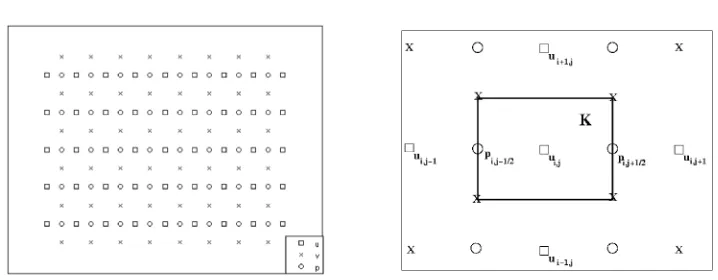
Figure 1. (a) Staggered grid, (b) a cellK corresponding to the first velocity componentu.
We use the Stokes equations and differentiate with respect toy:
∂y(∂xp˜n1+1) =− 1
2(∂y(∂xp
n
1)−∂y(∂xpn2)).
Applying again the Stokes equations, we end up with the second interface condition of (5.4):
∂xL3˜v1n+1=− 1
2ν(∂xL3v
n
1 −∂xL3vn2).
Thus, everything is shown.
Remark 5.3. The algorithm decouples into two scalar problems. Since one knows that each of these scalar algorithms converges in at most two steps, we obtain convergence in two steps for the three-dimensional case, too.
Remark 5.4. The new algorithm for the Stokes system is reminiscent of the hybrid approach presented in [10]. Indeed, in both cases, the interface conditions are mixed Dirichlet and Neumann type boundary conditions. But, our approach is different in two ways:
• It shows what is the good combination of stress and displacement for the interface conditions in both 2D and 3D.
• In the non-symmetric case, the complex interface condition (4.4) is not of the hybrid type as defined in [10].
6. Discretization
(a) (b) (c)
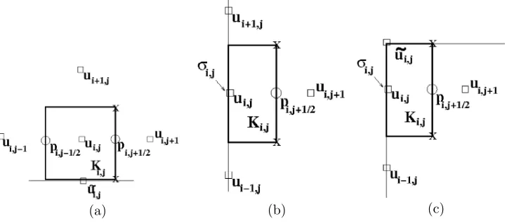
Figure 2. Boundary cells foru: (a) horizontal boundary cell, (b) vertical boundary cell, (c) corner cell.
centerxi,j (position ofui,j). Using integration by parts we obtain
Kij
f1dx =
Kij
(−ν∆u+cu+∂xp)dx
=
∂Kij
−ν∂nKiju+pnij,1
ds+
Kij
cudx
where nij,k is the k-th component of the outward normal nij of Kij. Now this
equation is discretized. We replace the derivatives of u by corresponding central differences and approximate the remaining integrals by the midpoint rule. For the pressure we assume that it is constant along the edges. We denote the length of an interior cellKij inx-direction by ∆xand the length iny-direction by ∆y.
For an interior cellKij we obtain the following equation:
∆x∆y f(xi,j) = ∆x∆y cui,j+ ∆y(−pi,j−1/2+pi,j+1/2)
+∆y
∆x ν(2ui,j−ui,j+1−ui,j−1)
+∆x
∆y ν(2ui,j−ui−1,j −ui+1,j).
(6.1)
The different cells at the boundary are plotted in Figure 2. One has to distinguish between cells connected to horizontal boundaries or vertical boundaries and corner cells. Let us start with the cells that are connected to the horizontal boundaries. In the new domain decomposition method there are interface conditions for the normal stress. Since the normal stress on a boundary edge cannot be computed directly, we have to introduce an artificial value ˜ui,j. Then, the stress on the horizontal
boundary can be approximated byνu˜i,j−ui,j
∆y/2 . Therefore, we obtain for the cell in Figure 2(a) the following modification of equation (6.1):
∆x∆yf(xi,j) = ∆x∆y cui,j+ ∆y(−pi,j−1/2+pi,j+1/2) +∆y
∆x ν(2ui,j−ui,j+1−ui,j−1) +
∆x
∆y ν(ui,j−ui+1,j) +
∆x
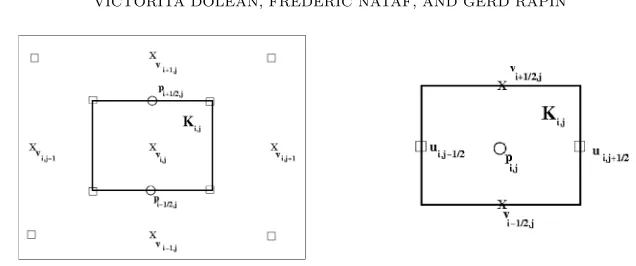
Figure 3. (a) Interior cell for the second velocity component v, (b) cell for the pressurep.
Next we consider a vertical boundary cell. Now, the cellKij is given by a half cell;
cf. Figure 2(b). We introduce on the boundary an artificial unknown σi,j for the
normal stress. Then the discretization is given by ∆x
2 ∆yf(xi,j) = ∆x
2 ∆y cui,j+ ∆y pi,j+1/2 +∆y
∆x ν(ui,j−ui,j+1) + ∆y σi,j+
∆x/2
∆y ν(2ui,j−ui−1,j−ui+1,j).
The corner cells are the combination of horizontal and vertical cells; cf. Figure 2 (c): ∆x
2 ∆yf(xi,j) = ∆x
2 ∆y cui,j+ ∆y pi,j+1/2 +∆y
∆x ν(ui,j−ui,j+1) + ∆y σi,j+
∆x/2
∆y ν(ui,j−ui−1,j) +
∆x/2
∆y/2 ν(ui,j−u˜i,j). Thus, for each cell ofuwe obtain one equation.
For the equation of the second velocity component v we proceed in a similar manner. The center of the cells for v are always given by the second velocity component. In Figure 3(a) an interior cell is plotted and in Figure 4 you can see, how the boundary cells can be treated.
The third equation is discretized with the help of the pressure nodes. Considering the cells centered by the pressure nodes, we observe that all cells can be handled in the same way; cf. Figure 3(b). Integrating over an arbitrary cellKij yields
0 =
∂Kij
unij,1+vnij,2ds,
where nij,k is the k-th component of the outward normal nij of Kij. Thus, the
discretization is given by
0 = ∆y(−ui,j−1/2+ui,j+1/2) + ∆x(−vi−1/2,j+vi+1/2,j).
Remark 6.1. In the correction step the pressure is only determined up to a constant. In order to avoid singular problems, we regularize the pressure equation by
0 = ∆y(−ui,j−1/2+ui,j+1/2) + ∆x(−vi−1/2,j+vi+1/2,j) +pi,j
(a) (b) (c) Figure 4. Boundary cells forv: (a) horizontal boundary cell, (b) vertical boundary cell, (c) corner cell.
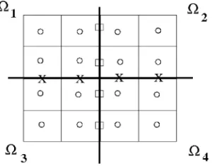
Figure 5. A 2×2 decomposition with pressure cells.
Finally, we discuss, how boundary conditions are imposed. Again, we restrict ourselves to the case of the first velocity component u. The boundary conditions for v are imposed analogously. On vertical boundaries Dirichlet conditions, re-spectively, Neumann conditions are imposed by simply setting the nodes for u, respectively, cσi,j on the interface. For horizontal boundaries Dirichlet conditions
are imposed by setting the artificial values ˜ui,j. A Neumann conditionν∂nu=gis
discretized by setting
(6.2) g(xi,j) =ν ∂u
∂n(xi,j)≈ν
˜
ui,j−ui,j
∆y/2
for all nodesxi,j corresponding to the artificial unknowns ˜ui,j (cf. Figure 2(b)).
For the domain decomposition we split the global rectangle Ω into local rectangles Ωi in such a way that we retrieve local subdomains with the above pattern. This
[image:19.612.233.383.295.413.2]be switched. Thus, in the correction step (3.14) a Dirichlet condition (6.3) u˜ni+1=−1
2(u
n i −u
n j)
for the first velocity componentuand a Neumann condition (6.4) σiτ
i(
˜
uni+1,p˜ni+1) =−1 2(σ
i τi(
˜
uni, pni) +σjτ
j(u
n j,p˜
n j))
for the second component v has to be imposed in subdomain Ωi. Neumann
con-ditions can be imposed following the line of (6.2), where normal derivatives of the right hand side of (6.4) can be computed by finite differences. For the Dirichlet conditions we just set the values on the interface to the corresponding value using the interface Dirichlet data of adjacent subdomains.
In the update step (3.15) we have a Neumann condition for the first velocity component and a Dirichlet condition for the second component. Imposing the Neumann condition for the first component is simple. One just sets the artificial stress σi,j on the interface to the given value using the artificial stresses on the
interface of the correction step. For the Dirichlet condition the artificial unknowns of the second velocity component on the interface are used.
We consider two different types of domain decomposition methods. First, we apply directly the discrete version of Algorithm 3.7. In the second version we have accelerated the algorithm using a Krylov method. Due to the non-symmetric structure of the boundary conditions we apply the GMRES method [25].
7. Numerical results
In this section we will analyze the performance of the new algorithm. It will be compared with the standard Schur complement approach using a Neumann-Neumann preconditioner (without coarse space); cf. [26]. We will extend the preliminary results of [4], where we made some numerical experiments for the two subdomains case, using standard inf-sup stable P2/P1-Taylor-Hood elements on triangles.
We consider the domain Ω = [0.2,1.2]×[0.1,1.1] decomposed into two or more subdomains of equal or different sizes. We choose the right hand side f such that the exact solution is given by u(x, y) = sin(πx)3sin(πy)2cos(πy), v(x, y) = −sin(πx)2sin(πy)3cos(πx) andp(x, y) =x2+y2. The viscosityν is always 1. We solve the problem for various values of the reaction coefficientc, which can arise for example, when one applies an implicit time discretization of the unsteady Stokes problem (c= 1/∆t).
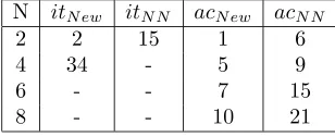
First, the interface system is solved by a purely iterative method (denoted re-spectively by itN ew and itN N for the new algorithm and the Neumann-Neumann
preconditioner) and then accelerated by GMRES (denoted respectively by acN ew
and acN N for the new algorithm and the Neumann-Neumann preconditioner). In
all tables we count the number of iterations needed to reduce theL∞ norm of the error by the factorT OL= 10−6:
max
i=1,...,Nu i
k−uhL∞(Ωi)≤10−6,
whereuik is the discrete solution of iteration stepkin subdomain Ωi anduhis the
Table 1. Two subdomains case: (a) Influence of the reaction pa-rameter on the convergence (h= 1/96). (b) Influence of the mesh size forc= 10−5.
c itN ew itN N acN ew acN N
102 2 15 1 6
100 2 15 1 6
10−3 2 15 1 6
10−5 2 15 1 6
h itN ew itN N acN ew acN N
1/24 2 14 1 6
1/48 2 15 1 6
1/96 2 15 1 6
Table 2. Two subdomains case: Influence of the length of the first domain: (a)c= 10−5,h= 1/100, (b)c= 1.0,h= 1/100.
L1/L itN ew itN N acN ew acN N
0.1 - - 7 8
0.2 22 22 5 7
0.3 5 16 3 6
0.4 5 15 3 6
0.5 2 15 1 6
L1/L itN ew itN N acN ew acN N
0.1 - - 7 8
0.2 15 18 5 7
0.3 5 16 3 6
0.4 5 15 3 7
0.5 2 15 1 6
Since the interface problem is ill-conditioned especially in the presence of cross-points, the reduction of the Euclidean norm of the residual is not a good indicator for the convergence of the algorithm. The case where the algorithm does not converge within 100 steps is denoted by−.
7.1. Two subdomains case. We first consider a decomposition into two
subdo-mains of same width and study the influence of the reaction parameter and of the mesh size on the convergence. We can see in Table 1(a) that the convergence of the new algorithm is optimal. For the iterative version convergence is reached in two iterations. Since in this case the preconditioned operator for the corresponding Krylov method reduces in theory to the identity, the Krylov method converges in one step. This is also valid numerically. Moreover, both algorithms are completely insensitive with respect to the reaction parameter. The advantage in comparison to the Neumann-Neumann algorithm is obvious.
In Table 1(b) we fix the reaction parameter c = 10−5 and vary the mesh size. The conclusions are similar: both algorithms converge independently of the mesh size and, again, we observe a clearly better convergence behavior of the new algo-rithm. The same kind of results are valid for different values ofc (not presented here).
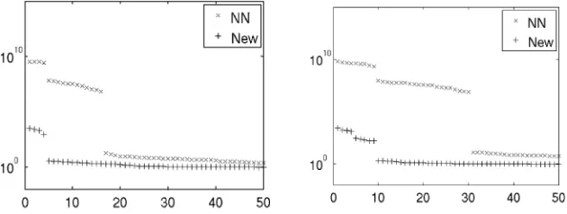
Next, we consider a decomposition into two subdomains where the first subdo-main is thinner than the second one. We study the influence of the ratio between the lengthL1 of the first subdomain and the global domainLfor three values ofc (see Tables 2, 3).
We observe that the iterative counterparts of the algorithms are very sensitive to the size of the first subdomain (it might not even converge when the parametercis very small), but as expected not the accelerated one. Second, when the parameter
[image:21.612.128.490.274.350.2]